Energy balancing of covariate distributions
-
Jared D. Huling
 und
Simon Mak
und
Simon Mak

Abstract
Bias in causal comparisons has a correspondence with distributional imbalance of covariates between treatment groups. Weighting strategies such as inverse propensity score weighting attempt to mitigate bias by either modeling the treatment assignment mechanism or balancing specified covariate moments. This article introduces a new weighting method, called energy balancing, which instead aims to balance weighted covariate distributions. By directly targeting distributional imbalance, the proposed weighting strategy can be flexibly utilized in a wide variety of causal analyses without the need for careful model or moment specification. Our energy balancing weights (EBW) approach has several advantages over existing weighting techniques. First, it offers a model-free and robust approach for obtaining covariate balance that does not require tuning parameters, obviating the need for modeling decisions of secondary nature to the scientific question at hand. Second, since this approach is based on a genuine measure of distributional balance, it provides a means for assessing the balance induced by a given set of weights for a given dataset. We demonstrate the effectiveness of this EBW approach in a suite of simulation experiments, and in studies on the safety of right heart catheterization and on three additional studies using electronic health record data.
1 Introduction
Studying the causal effect of a treatment or intervention is a central goal in many scientific disciplines. In randomized controlled trials, estimation of causal effects is possible since randomization ensures that treated units and control units are comparable [1]. However, for many pressing questions, it is impossible or impractical to randomize treatment assignments. Researchers are thus left with existing sources of observational data to answer these questions. In these observational studies, it is of prime interest to make unconfounded comparisons between treatment groups, a common example being estimation of the average treatment effect (ATE). Yet in observational settings, natural selection processes into the treatment, resulting in imbalance in the covariate distributions between treatment groups. This may then introduce substantial bias in naive comparisons of the outcome of interest between groups.
In observational studies based on complex electronic health records (EHRs) or administrative health data, the differences between treated and untreated units are typically substantial and difficult to characterize. One motivating application for our work is the study by Connors et al. [2], which explored the impact of right heart catheterization (RHC), a diagnostic procedure designed to guide therapy, on mortality among intensive care unit (ICU) patients. In this study, patients who received RHC are different from those who did not receive RHC in highly complex ways. As an example among many such differences, both younger patients and older patients are less likely to receive RHC; thus, a simple correction for the average age does not characterize the differences between those who received RHC and those who did not. Similar complex differences between treated and untreated patients can also be observed in three other motivating studies arising from clinical care and EHRs using the MIMIC-III critical care database [3]; we will demonstrate how the proposed method tackles these four challenging applications later.
There is a vast literature on adjustment methods for correcting for imbalances between treated and untreated units to reduce estimation bias in treatment effects. Weighting methods are a class of adjustment methods that control for confounding by re-weighting the treatment and control groups to look similar. Inverse-probability weighting (IPW) methods [4–9], which have origins in survey sampling, are by far the most commonly used weighting approaches. IPW methods model the treatment assignment mechanism (or propensity score, see Rosenbaum and Rubin [10]), and inverse weight each sample by the probability of receiving its assigned treatment. Inverse weighting by the true underlying propensity score controls for confounding, as it re-weights the covariate distributions of the treatment groups to that of the overall population.
In practice, IPW methods require positing and fitting a model for the propensity score. While model fitting is no unfamiliar task for a statistician, it has been noted in the literature that even mild model misspecifications for the propensity score can result in substantial bias in estimating the treatment effect [11]. Hearkening to George Box’s maxim, “all models are wrong, but some are useful,” it is often quite difficult in practice to obtain a useful propensity score model, especially in the presence of many covariates. Recent work has focused on mitigating this issue, by either (i) including conditions on the estimation of the propensity model which encourage moment balance of the covariates [12] or by (ii) altogether avoiding direct modeling of the propensity score and instead estimating weights that explicitly balance moments of the covariates either exactly [13,14] or approximately [15]. A large class of such estimators is explored Chan et al. [14] and further expanded on by Zhao [16] and has a long history [17]. Recent works [18,19] have attempted to mitigate this issue by focusing on nonparametric approaches to moment balancing, yet they require a careful choice of kernel function and tuning of multiple hyperparameters.
To make progress in addressing these issues, we show in this article that estimation bias for the ATE has a link to imbalance in the covariate distributions. This shows that balancing the full covariate distributions (and not just lower order moments) of the treatment groups to the full population provides a robust way for mitigating confounding. Although this is understood in the literature [16,20], in this article, we establish and make use of this link in a general manner, by (i) introducing a metric that evaluates how well a set of weights mitigates imbalance for a given dataset and (ii) developing a new method for estimating weights by minimizing this metric, yielding good distributional balance for a given dataset. The distributional balancing property of these weights allows for robust empirical performance; they tend to perform well in practice without relying on modeling assumptions for the propensity score or which moments are imbalanced. Our approach is designed to yield good distributional balance between treatment groups without the need of carefully tuning hyperparameters. Hirshberg et al. [21] study the theoretical properties of use of integral probability metrics for construction of weights; however, our work focuses on a specific choice that is suitable to wide use in practice. Despite the lack of need for tuning, our proposal works well empirically in a wide variety of settings.
We introduce weights that are explicitly constructed to balance the covariate distributions of the treatment groups to a target distribution (usually the full population). We do so by leveraging the energy distance presented in Székely and Rizzo [22]. The energy distance is a measure based on powers of the Euclidean distance and was originally introduced as a means to replace standard nonparametric goodness-of-fit tests in high dimensions. The energy distance has an exact duality with a norm on the characteristic functions, enabling its use to compare two (or more) distributions or the distributions of two samples. We show that a weighted energy distance still retains this duality, making it a rigorously justified and reliable metric to compare between multiple sets of weights for a given dataset. From this, we propose the so-called energy balancing weights (EBWs), which are defined as the weights which minimize the weighted energy distance between treatment groups and the full sample, subject to constraints that mitigate variability in the weights. We prove that EBWs asymptotically ensure full distributional balance and result in root-
Although we focus primarily on a simple estimand, namely, the average treatment effect (ATE) the proposed weights can be used for a wide variety of causal estimands since the distributional re-balancing property of EBWs enables flexible control of confounding. We show that they can be used for the estimation of a wide variety of causal quantities, such as the ATE and individualized treatment rules (ITRs) [23,24]. With minor modifications, they can also be used for estimation of the average treatment effect on the treated (ATT) and for estimating treatment effects for multi-category treatments. Despite the fact that EBWs are not specifically designed to match low-order moments, in practice, they often result in better marginal mean balance of covariates than propensity score methods even in high dimensions (50–100 covariates), as seen in Section 6. EBWs are also quite stable in practice, rarely resulting in large weights, an issue that plagues standard propensity score methods [11], making it less critical to impose constraints that induce weight variability. EBWs are constructed without using outcome information; however, as for other weighting approaches, variance can be reduced via augmented estimators that make use of outcome regression models, such as the augmented estimators in the studies by Wong and Chan [18], Zhao [16], and Athey et al. [25]. However, we do not explore such techniques here.
The remainder of this article is organized as follows. Section 2 motivates the need for distributional balance and introduces the weighted energy distance. Section 3 presents the proposed EBWs and discusses their computation and asymptotic properties. Section 5 compares the performance of EBWs with other weighting methods in simulation studies. Section 6 discusses an application of EBWs in a study of RHC and further uses these data to explore highly challenging simulations that use the natural data-generating processes of the study. Section 7 further demonstrates the utility of EBWs by analyzing data from a complex application involving EHR data. Section 8 concludes with a discussion and future work.
2 Distributional balance and weighted energy distance
2.1 Setup
Consider a sample
Let us denote
Using the notation of potential outcomes, the (population) ATE is defined as
where
2.2 Weighted average estimates and distributional balance
We restrict our focus to weighted averages as estimates of the ATE. Given a vector of weights
The most commonly used example of (2), inverse propensity score weighting, uses
Given any weight vector
where
The notion that the covariate distributions should be balanced to obtain a good estimate of
2.3 Weighted energy distance
We introduce next a new measure of the distributional balance induced by a set of weights. This measure is based on the energy distance, which is a metric on distributions [34]. Due to the link between estimation bias and distributional imbalance, our measure can be used to evaluate the degree of bias one expects from a given set of weights and a given dataset. We will later leverage this measure to construct distributional balance weights that minimize this metric for a given dataset.
The energy distance (as surveyed in Székely and Rizzo [34]) is defined as follows. Let
where
The energy distance has been used within a wide variety of statistical methods, e.g., for testing equivalence of distributions, for testing statistical independence [35], and for generating samples from a target distribution [36]. The energy distance is simple to compute as it only involves sums of Euclidean distances, it is nonnegative, and it can be shown to be equivalent to a distance between the characteristic functions of
We propose a weighted modification of this energy distance, which measures the distance between a weighted distribution, i.e., the weighted covariate ECDFs
In other words,
We show this new weighted energy distance is indeed a distance between
respectively. The following proposition establishes the distance property of the weighted energy distance.
Proposition 2.1
Let
where
Thus, the weighted energy distance is a distance between the weighted distribution of interest and the target distribution, and is thus a bona fide measure of distributional balance of covariates induced by a set of weights. This proportion extends the duality results of Proposition 1 from Székely and Rizzo [34] and Theorem 1 from Székely et al. [35] for the weighted energy distance at hand. A subtle point is that Proposition 2.1, combined with the decomposition presented in Section 2.2, makes clear that
We now show that the weighted energy distance converges to the energy distance when the weights yield a well-defined limiting distribution.
Theorem 2.2
Assume
Theorem 2.2 shows that the weighted energy distance converges to the limiting energy distance. If the limiting distribution implied by a set of weights is
2.4 Bias and distributional imbalance
We now demonstrate this connection between bias and distributional imbalance (as measured by the weighted energy distance) using two illustrative examples. A more formal presentation is provided later in Section 3.2 when proving asymptotic properties of EBWs.
In the first illustrative example, we generate a one-dimensional covariate of sample size 250, which impacts treatment assignment via a logistic model under each of three scenarios: (1)
Figure 1(a) displays the energy distances and biases over 1,000 replications of the experiment. We see that the energy distances are the largest in all scenarios for the unweighted estimator ((2) with all weights equal to 1). For scenarios where the weights are estimated using a misspecified model (IPW (1) in Scenario 2 and IPW (1) and (2) in Scenario 3), the energy distances are much larger than for weights based on correctly (or over-specified) models. Correspondingly, the bias is pronounced for the misspecified models. Thus, the weighted energy distance can be a useful tool to compare between different models, as weights with smaller weighted energy distances tend to yield estimates with smaller error.
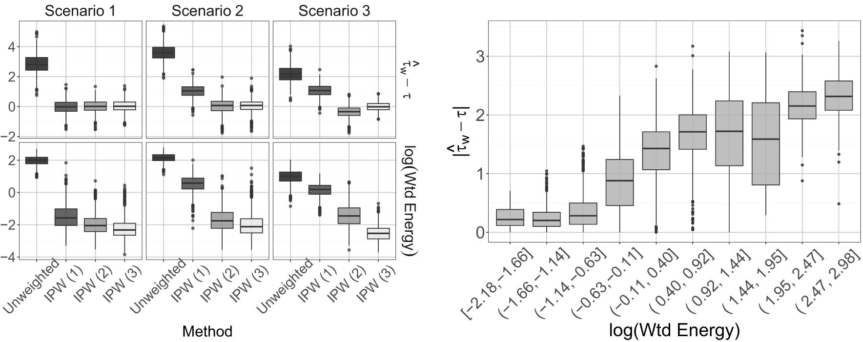
(a, left) Energy distances and biases for IPW estimates based on weights from the three fitted logistic regression models; (b, right) Boxplots of the biases for IPW estimates versus weighted energy distance based on weights estimated by several methods, each with different combinations of moments included for balancing or estimation.
In the second example, we consider a two-dimensional example where the true assignment mechanism depends on first and second moments of the covariates. We consider several methods for estimate weights: logistic regression, the method of Imai and Ratkovic [12], and the method of Chan et al. [14], each with different moments included for balancing or estimation. We then compare their weighted energy distances and absolute errors of (2) over 1,000 replications. Figure 1(b) displays the distances and errors for each dataset and method. We see that, in general, weights with lower energy distance have a much smaller magnitude of bias in estimating the ATE.
2.5 Other measures of distributional imbalance
There are, of course, many ways of measuring distance between distributions in the literature, including the Kolmogorov-Smirnov statistic,
3 Energy balancing weights
3.1 Definition
We will now use the proposed weighted energy distance to estimate weights which (i) match the distribution of covariates of the treated group to the distribution of covariates of the full population, and (ii) match the distribution of covariates of the control group to the distribution of covariates of the full population.
To achieve this, we define the EBWs to be
Thus, the EBWs
To illustrate the effectiveness of EBWs for distributional balance, we consider data generated under Scenario 3 of the toy example in Figure 1(a). Figure 2 shows the difference between the weighted ECDF using EBWs of the covariate in the treatment group and the ECDF of the combined (i.e., treated and untreated) sample, for varying sample sizes

Displayed are the absolute differences between the ECDF of the combined sample and the weighted ECDF of the covariate in the treatment group based on energy weights. Also displayed the same for the unweighted ECDF of the treated group and the weighted ECDF based on the true and estimated propensity scores.
EBWs can be naturally extended to handle a wide variety of scenarios, such as for treatments with more than two levels, estimation of the ATT, and for the estimation of optimal ITRs. In the Supplementary Material, we show how these extensions are manifested and empirically demonstrate the benefit of using EBWs for ITR estimation.
A few key distinguishing features of our proposal from the works of Wong and Chan [18] and Kallus [19] are (1) its direct focus on distributional balance rather than moment balance. Despite the connection between balancing moments of an infinite dimensional class of functions and distributional balance, this feature helps alleviate modeling decisions about what moments to balance of what space of moments to balance and has advantages in terms of interpretability and (2) by focusing on a measure that does not require tuning parameters to characterize distributional differences, our approach can be applied broadly by practitioners of varying degrees of statistical sophistication.
3.2 Asymptotic properties
Next, we show two desirable properties of the proposed EBWs. We first show that the weighted ECDFs based on EBWs indeed converge to the population CDF
Theorem 3.1
Assume that
almost surely for every continuity point
holds almost surely.
Thus, EBWs result in the almost sure convergence of the weighted ECDFs of the treated (and untreated) group to the underlying covariate distribution
The consistency of
Corollary 3.2
Suppose the conditions of Theorem
3.1
hold, and that the treatment and control mean response functions
Next, we show that the ATE estimator
Lemma 3.3
Let
where
Lemma 3.3 provides a connection between the systematic bias in (3) and the weighted energy distance
Theorem 3.4
Assume the same conditions in Theorem
3.1. Let
- (12)
The EBWs
We give a brief discussion of Assumptions (A1)–(A5). Assumption (A1) concerns the regularity of the conditional mean functions
While Theorem 3.4 proves the desired root-
3.3 Optimization
The optimization problem (10) for computing EBWs (and the later optimization problem (16) for obtaining three-way EBWs) can be viewed as quadratic programs with linear (in)equality constraints. There has been much work on efficient algorithms for solving such programs [41], including interior point methods [42], augmented Lagrangian techniques [43], and extensions of the simplex algorithm [44]. A recent development is the operator splitting approach in Stellato et al. [45], which provides a reliable alternative for nonpositive definite quadratic programs.
In our implementation, we made use of well-maintained interior-point cone programming solvers in the R package cccp [46] for optimizing the EBW formulations (10) and (16). Such solvers follow a two-stage procedure: finding an initial feasible solution for
3.4 Controlling weight variability
In our experience, the weights resulting from the optimization criterion (10) rarely, if ever, result in large weights; however, in the literature there has been an emphasis on methods that afford explicit control on the variability of weights [33]. To allow for such within our framework, one can simply add a penalty
3.5 Three-way EBWs
The EBWs in (10) are designed to balance the distributions of covariates between each treatment group to that of the combined sample
Terms (14) and (15) shed light on how the choice of
We propose an extension of EBWs, the improved EBWs (iEBWs), to help improve covariate balance between the treatment and control groups. These improved weights are defined as follows:
where
is the energy distance between the weighted ECDFs for treated and control. Thus, the iEBWs
4 Extensions and applications of EBWs
4.1 Estimation of the ATT
A common target of estimation is the (population) ATT,
which suggests that a plug-in estimator can be obtained by replacing
where
4.2 Multi-category treatments
EBWs can also be constructed for multi-category treatments. When the treatment
We define the EBWs for the multiple treatment case as follows:
Improved EBWs, which encourage covariate balance between all pairs of treatment options, can be defined similarly as (16), where an additional weighted energy distance between each pair of treatment options is added to the objective. Given any two treatment options
4.3 Estimation of ITRs
As many treatments exhibit heterogeneous effects for different patients, there is great interest in tailoring treatment decisions to patients. A main line of work in this area is the development of statistical methods aimed at finding an optimal ITR, which maps patient characteristics to treatment decisions. Thus, the immediate goal is to estimate a mapping
where
Due to the nonconvexity of (20), in practice
where
To demonstrate the effectiveness of using EBWs in optimal ITR estimation, we provide an illustrative example under two data-generating scenarios. For both scenarios, we generate outcomes as
Displayed are the value functions and misclassification rates for the optimal ITR estimation example averaged over 1,000 independent simulated datasets
| Scenario 1 | Scenario 2 | |||||
|---|---|---|---|---|---|---|
| Method | Value (SD) | Misclass | Value (SD) | Misclass | ||
| OWL (EBW) | 3.168 | (0.253) | 0.283 | 2.921 | (0.166) | 0.228 |
| OWL (iEBW) | 3.198 | (0.204) | 0.277 | 2.931 | (0.165) | 0.223 |
| OWL (PS) | 2.671 | (0.327) | 0.344 | 2.706 | (0.196) | 0.295 |
In Scenario 1, the optimal value is 4.74 with 56% of units with optimal assignments of
5 Simulation studies
To evaluate the finite sample performance and operating characteristics of our proposed estimators, we conducted a large-scale simulation study across a wide variety of data-generating scenarios. Since existing techniques, such as empirical calibration balancing and the covariate balancing propensity score, work exceedingly well when the correct moments are specified to be balanced, we primarily consider simulation settings where the relationships between covariates and both the treatment status and outcome regression model are nonlinear. We consider a wide range of scenarios for the propensity score and outcome regression models, several of which are examples taken from the existing works. Outcome models B and E are taken from [18], outcome model D is taken from Wong and Chan [50], and outcome model A is a slight modification of an outcome model from Kang and Schafer [11]. Outcome model C is designed to be linear in
We compare our proposed EBW and the iEBWs (16), both with no penalty on the squares of the weights, with several widely used alternatives. First, we compare with inverse propensity score weights (denoted “IPW”). In addition, we compare with the covariate balancing propensity score weights (denoted “CBPS”), the empirical calibration balancing weights (denoted “Cal”) with exponential tilting weights. For all methods that require specification of a model for the treatment assignment or moments to balance, only first-order terms in
For the sake of brevity of presentation, we present a summary of the results across all outcome models. More detailed results are presented in the Supplementary Material. Table 2 contains a summary of the results averaged across outcome models (A–E) and dimension settings (
Displayed are the ranks among all methods tested of each method in terms of RMSE and bias averaged over all response models (I–VI) for
| Propensity model: | I | II | III | IV | V | VI | ||||||
|---|---|---|---|---|---|---|---|---|---|---|---|---|
| Mean rank | Mean rank | Mean rank | Mean rank | Mean rank | Mean rank | |||||||
| Method | RMSE | Bias | RMSE | Bias | RMSE | Bias | RMSE | Bias | RMSE | Bias | RMSE | Bias |
| Unweighted | 4.7 | 3.7 | 6.5 | 4.9 | 5.0 | 4.5 | 4.8 | 4.1 | 6.2 | 5.3 | 3.9 | 3.1 |
| EBW | 2.5 | 2.8 | 2.4 | 2.7 | 3.2 | 4.2 | 2.5 | 3.6 | 1.9 | 2.6 | 2.5 | 3.8 |
| iEBW | 2.2 | 2.5 | 1.5 | 1.7 | 3.0 | 3.9 | 1.7 | 3.5 | 1.9 | 2.0 | 2.0 | 3.1 |
| KCB | 3.0 | 3.4 | 2.5 | 2.5 | 3.2 | 4.3 | 2.7 | 2.5 | 3.0 | 3.6 | 2.5 | 2.3 |
| IPW | 5.5 | 5.0 | 6.4 | 5.9 | 5.0 | 2.9 | 6.3 | 5.4 | 5.8 | 5.1 | 6.8 | 6.0 |
| CBPS | 5.1 | 4.8 | 5.1 | 5.3 | 4.7 | 3.9 | 5.1 | 3.7 | 5.6 | 5.3 | 4.9 | 4.2 |
| Cal | 5.0 | 5.8 | 3.6 | 5.0 | 3.9 | 4.3 | 4.9 | 5.2 | 3.6 | 4.1 | 5.4 | 5.5 |
6 RHC data
6.1 Description of data
A study by Connors et al. [2] was conducted to investigate the effectiveness of RHC, a diagnostic procedure for critically ill patients in ICUs. Since RHC is more relevant for certain forms of intensive care than others, there is substantial imbalance in patient characteristics in those treated with RHC and those who did not receive RHC. The original analysis was based on propensity score matching, and the data have been subsequently re-analyzed in many other works [7,20,52,53]. The study consists of data on 5,735 individuals, 2,184 of whom received RHC, and the remaining 3,551 did not receive RHC. The outcome is an indicator of survival at 30 days after admission. A panel of experts convened to discuss which variables contribute to a decision to use RHC, resulting in a large set of covariates to study (72 in total, 21 of which are continuous, 25 binary, and 26 dummy variables originating from 6 categorical covariates). The dataset is publicly available at: http://biostat.mc.vanderbilt.edu/wiki/pub/Main/DataSets/rhc.html. There are substantial empirical differences in the distributions of many of these covariates between treatment groups (RHC vs. no RHC). In Section 6.2, we study the effect of RHC on 30-day survival. However, since there is no ground truth available, in Section 6.3, we use the RHC data to conduct a realistic simulation that demonstrates the effectiveness of EBWs.
6.2 Analysis of RHC data
We used 65 of the available covariates, as in the analysis of the same dataset in Rosenbaum [53], leaving out date-related covariates. Using the 65 covariates, we applied the weighting methods used in Section 5 (except the method of Wong and Chan [18] as the code returned constant weights of 1 regardless of the tuning parameters used) to estimate weights to balance the treated groups. To first investigate how well each method balances the marginal means of each covariate, we evaluate the absolute standardized mean differences for each covariate and
Displayed are
![Figure 4
This figure illustrates the differences in the marginal univariate weighted ECDFs between the treated and control populations. In particular, let
x
j
∈
X
j
{x}_{j}\in {{\mathcal{X}}}_{j}
denote the
j
j
component of the covariate vector
x
{\bf{x}}
and let
F
n
,
a
,
j
(
x
)
{F}_{n,a,j}\left(x)
denote its empirical CDF on treatment arm
a
a
. Similarly denote the weighted versions of this quantity. Here, we are displaying how well each method balances the marginal empirical CDFs for the treated and control arms. We do so by evaluating an estimate of
∫
x
j
∈
X
j
[
F
n
,
1
,
j
,
w
‒
F
n
,
0
,
j
,
w
]
(
x
j
)
d
x
j
1
∕
2
{\left\{{\int }_{{x}_{j}\in {{\mathcal{X}}}_{j}}{[}{F}_{n,1,j,{\boldsymbol{w}}}‒{F}_{n,0,j,{\boldsymbol{w}}}]\left({x}_{j}){\rm{d}}{x}_{j}\right\}}^{1/2}
obtained by integration over a grid of values for all
j
=
1
,
…
,
65
j=1,\ldots ,65
. The results across all covariates are displayed in the left two plots above. The rightmost plots similarly display the RIMSEs for all possible 65 choose 2 bivariate CDFs.](/document/doi/10.1515/jci-2022-0029/asset/graphic/j_jci-2022-0029_fig_004.jpg)
This figure illustrates the differences in the marginal univariate weighted ECDFs between the treated and control populations. In particular, let
Estimates of the ATE and standard errors for the RHC data. Standard errors were computed for all methods using the nonparametric bootstrap with 1,000 replications. Also displayed are various measures of discrepancy between the distributions of covariates for the RHC and non-RHC groups. In addition to weighted energy distances, we display mean and max “
| Unwtd | CBPS | IPW | Cal | EBW | iEBW | |
|---|---|---|---|---|---|---|
|
|
0.0736 | 0.0576 | 0.0528 | 0.0547 | 0.0499 | 0.0470 |
| SE
|
0.0132 | 0.0142 | 0.0155 | 0.0145 | 0.0120 | 0.0117 |
| Energy dist (10) | 8.1996 | 0.8572 | 0.7804 | 0.4250 | 0.3236 | 0.3377 |
| Energy dist (16) | 23.7172 | 1.8560 | 1.5756 | 1.0045 | 0.7536 | 0.7270 |
| Mean
|
0.1648 | 0.0274 | 0.0182 | 0.0000 | 0.0063 | 0.0043 |
| Max
|
0.5826 | 0.1139 | 0.0778 | 0.0000 | 0.0239 | 0.0168 |
| SD
|
0.1276 | 0.0206 | 0.0147 | 0.0000 | 0.0050 | 0.0036 |
6.3 RHC data simulation
In this section, we fix the covariates and treatment assignments from the RHC data, and simulate responses with confounding. This produces a realistic and highly challenging simulation scenario with high dimension. We use the key functional form from outcome model D from Section 5. Since this outcome model involves only 7 covariates, we use the functional form from this outcome model, apply it over 8 separate groups of 7 covariates in the RHC data, and take the sum of all groups of 7 covariates as the mean of the outcome. We then simulate 1,000 independent datasets using this procedure and each time estimate the ATE and record each method’s RMSE in estimating the true ATE. Since under this model the ordering of the covariates changes the nature of the confounding, we randomly permute the columns 100 times and repeat the simulation 1,000 times for each permutation and each time record the RMSE over the 1,000 replications. Further details are provided in the Supplementary Material. The RMSEs for each of the 100 column permutations are displayed in Figure 5. Both EBW and iEBW consistently yield among the smallest RMSE across the permutation settings. Since the outcome model in this simulation involves a constant treatment effect, and thus is not impacted by potential issues of covariate overlap, and in the Supplementary Material, we additionally consider an outcome model with a treatment effect that depends on
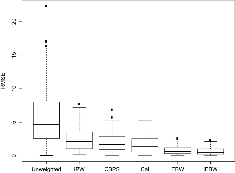
RMSEs for each method across 100 outcome models using the RHC data.
7 Analysis of the MIMIC-III critical care database
We analyze the effectiveness of three treatments based on separate subpopulations of the MIMIC-III v1.4 critical care database [3]: a study of the effect of indwelling arterial catheters (IACs) on mortality in patients with respiratory failure [54], a study of the effect of transthoracic echocardiography (echo) on mortality in sepsis patients [55], and a study of mechanical power of ventilation (MPV) on mortality in critically ill patients [56]. Each study is based on the existing studies utilizing MIMIC-III. The degree of confounding in each study varies, with the IAC and MPV studies exhibiting a great degree of confounding and the echo study with minimal confounding. For all studies, missing values were imputed using missForest [57]. We present the IAC study in this section and the remaining two studies in the Supplementary Material. For each study, we present treatment effect estimates and balance statistics using each method used in the main text. For all studies, we also use the covariates and treatment assignments of the observed data to conduct simulation studies, using the same approach used for the simulation based on the RHC data. In essence, with these simulation studies we preserve the treatment assignment mechanism of the observed data and simulate outcomes that involve a high likelihood of confounding under this real-world treatment assignment mechanism. The simulation studies investigate scenarios with a constant treatment effect over
7.1 IAC data
In this section, we replicate a study originally conducted Hsu et al. [54] based on the MIMIC-III critical care database to study the effect of indwelling arterial catherization on 28 day mortality. The data are based on the queries provided in https://github.com/MIT-LCP/mimic-codeand contains information on 2,522 mechanically-ventilated patients, 1,298 of whom received the treatment, IAC. The outcome is an indicator of 28 day mortality from time of admission. Pre-treatment covariates likely to be confounders include demographics, lab values, calculated risk scores, missingness indicators, and more, totaling to a design matrix with
Estimates of the ATE and standard errors for the IAC data. Standard errors were computed for all methods using the nonparametric bootstrap with 1,000 replications. Also displayed are various measures of discrepancy between the distributions of covariates for the IAC and control groups. We also display the mean and max RIMSE statistic for marginal univariate and bivariate CDF differences, as in Figure 4. In addition, we display summary statistics of SMDs for marginal means and SMDs for all polynomials up to order 5 and pairwise interactions (denoted SMD(2)). The bold values indicate the best performance across all methods for a given setting
| Unweighted | CBPS | IPW | Cal | EBW | iEBW | |
|---|---|---|---|---|---|---|
|
|
0.0012 |
|
|
|
|
|
| SE
|
0.015 | 0.0217 | 0.0446 | 0.0165 | 0.0118 | 0.0114 |
| Energy dist (10) | 4.5625 | 0.7829 | 31.336 | 0.5612 | 0.3869 | 0.4028 |
| Energy dist (16) | 13.6796 | 1.6922 | 62.6704 | 1.3854 | 0.9614 | 0.9304 |
| Mean RIMSE, 1d | 0.0362 | 0.0130 | 0.0670 | 0.0126 | 0.0113 | 0.0111 |
| Max RIMSE, 1d | 0.0863 | 0.0277 | 0.1646 | 0.0256 | 0.0235 | 0.0245 |
| Mean RIMSE, 2d | 0.0416 | 0.0075 | 0.0619 | 0.0071 | 0.0067 | 0.0062 |
| Max RIMSE, 2d | 0.3295 | 0.0283 | 0.2028 | 0.0284 | 0.0248 | 0.0189 |
| Mean
|
0.0732 | 0.0023 | 0.0990 | 0.0001 | 0.0060 | 0.0045 |
| Max
|
0.2996 | 0.0203 | 1.2906 | 0.0028 | 0.0289 | 0.0212 |
| Mean
|
0.0788 | 0.0081 | 0.0932 | 0.0075 | 0.0093 | 0.0073 |
| Max
|
0.6801 | 0.1782 | 1.2906 | 0.1412 | 0.1502 | 0.0998 |
In addition, we conduct a simulation study based on the IAC data with precisely the same response-generating mechanism as for the simulation on the RHC data in Section 6.3. Although the dimension of the IAC data is higher, the number of dimensions that impact the response for each data-generating setting is 63, the same as in Section 6.3. The results in terms of RMSE in estimating the ATE across the 100 data-generating scenarios for both the constant and heterogeneous treatment effect settings, each averaged over 1,000 replications, are displayed in Table 5. The iEBW approach results in the smallest mean, median, and worst-case RMSE, followed by EBW, which is closely followed by Cal and CBPS. IPW in this case results in nearly worse performance than no weighting. We also conducted the same simulation study but with a treatment effect that varies in
Displayed are the median, mean, standard deviation, and maximum RMSEs for each method across the 100 simulation settings using the IAC data. The bold values indicate the best performance across all methods for a given setting
| Unweighted | CBPS | IPW | Cal | EBW | iEBW | |
|---|---|---|---|---|---|---|
| Constant treatment effect | ||||||
| Median RMSE | 8.0151 | 3.2899 | 7.9435 | 3.4895 | 3.0276 | 1.8319 |
| Mean RMSE | 9.1296 | 3.8542 | 9.5545 | 3.7609 | 3.5113 | 2.2087 |
| SD RMSE | 6.7091 | 2.5588 | 7.5263 | 2.5293 | 2.5028 | 1.5785 |
| Max RMSE | 32.3715 | 11.0479 | 39.1095 | 12.0521 | 12.4231 | 7.2066 |
| Heterogeneous treatment effect | ||||||
| Median RMSE | 11.9037 | 3.8587 | 15.1933 | 3.7128 | 3.0732 | 1.7355 |
| Mean RMSE | 13.5594 | 4.4330 | 18.4590 | 4.1689 | 3.9079 | 1.8688 |
| SD RMSE | 9.9665 | 3.1225 | 14.6490 | 2.8963 | 2.8718 | 1.3415 |
| Max RMSE | 48.0820 | 12.3672 | 75.3899 | 12.8563 | 13.8571 | 5.6715 |
8 Discussion
We have introduced a new metric, the weighted energy distance, which measures the distributional balance induced by a set of weights and thus can be used to determine which set of weights is likely to result in low bias when estimating a causal quantity. Building on the weighted energy distance, we have introduced the EBWs that minimize this distance to achieve distributional balance. The energy balancing weights are robust and reliable across many functional forms of confounding and further rarely result in large weights. Due to the distributional balancing of the energy balancing weights, they can be utilized to estimate a wide variety of causal estimands which can be represented as a statistical functional of the population distribution function of the covariates. While we focused entirely on the weighted energy distance, the connection between the energy distance and distances between embeddings of probability measures into reproducing kernel Hilbert spaces [39] opens up the possibility of more effective distributional balancing weights if more is known about the functional form of confounding. In particular, if the analyst believes lower order projections of the distribution should be balanced with priority over higher order aspects of the distribution, the use of a kernel which emphasizes these projections, such as the sparsity-inducing kernel in Mak and Joseph [58], could be used.
Acknowledgements
The authors would like to thank the anonymous referees for their helpful and constructive feedback. Dr. Mak was funded by NSF CSSI Frameworks 2004571, NSF DMS 2316012, and NSF DMS 2316012.
-
Conflict of interest: Authors state no conflict of interest.
References
[1] Dasgupta T, Pillai NS, Rubin DB. Causal inference from 2K factorial designs by using potential outcomes. J R Stat Soc Ser B (Stat Methodol). 2015;77(4):727–53. 10.1111/rssb.12085Suche in Google Scholar
[2] Connors AF, Speroff T, Dawson NV, Thomas C, Harrell FE, Wagner D, et al. The effectiveness of right heart catheterization in the initial care of critically Ill patients. J Amer Med Assoc. 1996;276(11):889–97. 10.1001/jama.276.11.889Suche in Google Scholar PubMed
[3] Johnson AE, Pollard TJ, Shen L, Li-wei HL, Feng M, Ghassemi M, et al. MIMIC-III, a freely accessible critical care database. Scientific Data. 2016;3:160035. 10.1038/sdata.2016.35Suche in Google Scholar PubMed PubMed Central
[4] Robins JM, Rotnitzky A. Semiparametric efficiency in multivariate regression models with missing data. J Amer Stat Assoc. 1995;90(429):122–9. 10.1080/01621459.1995.10476494Suche in Google Scholar
[5] Hahn J. On the role of the propensity score in efficient semiparametric estimation of average treatment effects. Econometrica. 1998;66:315–31. 10.2307/2998560Suche in Google Scholar
[6] Robins JM, Hernan MA, Brumback B. Marginal structural models and causal inference in epidemiology. Epidemiology. 2000;11:550–60. 10.1097/00001648-200009000-00011Suche in Google Scholar PubMed
[7] Hirano K, Imbens GW. Estimation of causal effects using propensity score weighting: An application to data on right heart catheterization. Health Services Outcomes Res Meth. 2001;2(3–4):259–78. Suche in Google Scholar
[8] Hirano K, Imbens GW, Ridder G. Efficient estimation of average treatment effects using the estimated propensity score. Econometrica. 2003;71(4):1161–89. 10.1111/1468-0262.00442Suche in Google Scholar
[9] Imbens GW. Nonparametric estimation of average treatment effects under exogeneity: A review. Rev Econom Stat. 2004;86(1):4–29. 10.1162/003465304323023651Suche in Google Scholar
[10] Rosenbaum PR, Rubin DB. The central role of the propensity score in observational studies for causal effects. Biometrika. 1983;70(1):41–55. 10.1093/biomet/70.1.41Suche in Google Scholar
[11] Kang JD, Schafer JL. Demystifying double robustness: A comparison of alternative strategies for estimating a population mean from incomplete data. Stat Sci. 2007;22(4):523–39. 10.1214/07-STS227Suche in Google Scholar PubMed PubMed Central
[12] Imai K, Ratkovic M. Covariate balancing propensity score. J R Stat Soc Ser B (Stat Methodol). 2014;76(1):243–63. 10.1111/rssb.12027Suche in Google Scholar
[13] Hainmueller J. Entropy balancing for causal effects: A multivariate reweighting method to produce balanced samples in observational studies. Political Analysis. 2012;20(1):25–46. 10.1093/pan/mpr025Suche in Google Scholar
[14] Chan KCG, Yam SCP, Zhang Z. Globally efficient non-parametric inference of average treatment effects by empirical balancing calibration weighting. J R Stat Soc Ser B (Stat Methodol). 2016;78(3):673–700. 10.1111/rssb.12129Suche in Google Scholar PubMed PubMed Central
[15] Zubizarreta JR. Stable weights that balance covariates for estimation with incomplete outcome data. J Amer Stat Assoc. 2015;110(511):910–22. 10.1080/01621459.2015.1023805Suche in Google Scholar
[16] Zhao Q. Covariate balancing propensity score by tailored loss functions. Ann Stat. 2019 Apr;47(2):965–93. 10.1214/18-AOS1698Suche in Google Scholar
[17] Deming WE, Stephan FF. On a least squares adjustment of a sampled frequency table when the expected marginal totals are known. Ann Math Stat. 1940;11(4):427–44. 10.1214/aoms/1177731829Suche in Google Scholar
[18] Wong RK, Chan KCG. Kernel-based covariate functional balancing for observational studies. Biometrika. 2017;105(1):199–213. 10.1093/biomet/asx069Suche in Google Scholar PubMed PubMed Central
[19] Kallus N. Generalized optimal matching methods for causal inference. J Machine Learn Res. 2020;21(1):2300–53. Suche in Google Scholar
[20] Li F, Morgan KL, Zaslavsky AM. Balancing covariates via propensity score weighting. J Amer Stat Assoc. 2018;113(521):390–400. 10.1080/01621459.2016.1260466Suche in Google Scholar
[21] Hirshberg DA, Maleki A, Zubizarreta JR. Minimax linear estimation of the retargeted mean. 2019. arXiv: http://arXiv.org/abs/arXiv:190110296. Suche in Google Scholar
[22] Székely GJ, Rizzo ML. Testing for equal distributions in high dimension. InterStat. 2004;5(1–6):1249–72. Suche in Google Scholar
[23] Qian M, Murphy SA. Performance guarantees for individualized treatment rules. Ann Stat. 2011;39(2):1180. 10.1214/10-AOS864Suche in Google Scholar PubMed PubMed Central
[24] Zhao Y, Zeng D, Rush AJ, Kosorok MR. Estimating individualized treatment rules using outcome weighted learning. J Amer Stat Assoc. 2012;107(499):1106–18. 10.1080/01621459.2012.695674Suche in Google Scholar PubMed PubMed Central
[25] Athey S, Imbens GW, Wager S. Approximate residual balancing: debiased inference of average treatment effects in high dimensions. J R Stat Soc Ser B (Stat Methodol). 2018;80(4):597–623. 10.1111/rssb.12268Suche in Google Scholar
[26] Neyman J. On the application of probability theory to agricultural experiments. Essay on principles. Section 9. translated in Statistical Science. vol. 1923; 1990. p. 465–472. Suche in Google Scholar
[27] Rubin DB. Estimating causal effects of treatments in randomized and nonrandomized studies. J Educ Psychol. 1974;66(5):688. 10.1037/h0037350Suche in Google Scholar
[28] Rubin DB. Bayesian inference for causal effects: The role of randomization. Ann Stat. 1978;6(1):34–58. 10.1214/aos/1176344064Suche in Google Scholar
[29] Hernan MA, Robins JM. Causal inference. Boca Raton, FL: CRC; 2019. Suche in Google Scholar
[30] Dawid AP. Some misleading arguments involving conditional independence. J R Stat Soc Ser B (Methodological). 1979;41(2):249–52. 10.1111/j.2517-6161.1979.tb01079.xSuche in Google Scholar
[31] Hájek J. Comment on a paper by D. Basu. Foundations of Statistical Inference; 1971. p. 236. Suche in Google Scholar
[32] Ding P, Li F. Causal Inference: A Missing Data Perspective. Stat Sci. 2018 May;33(2):214–37. 10.1214/18-STS645Suche in Google Scholar
[33] Chattopadhyay A, Hase CH, Zubizarreta JR. Balancing vs modeling approaches to weighting in practice. Stat Med. 2020;39(24):3227–54. 10.1002/sim.8659Suche in Google Scholar PubMed
[34] Székely GJ, Rizzo ML. Energy statistics: A class of statistics based on distances. J Stat Plan Inference. 2013;143(8):1249–72. 10.1016/j.jspi.2013.03.018Suche in Google Scholar
[35] Székely GJ, Rizzo ML, Bakirov NK. Measuring and testing dependence by correlation of distances. Ann Stat. 2007;35(6):2769–94. 10.1214/009053607000000505Suche in Google Scholar
[36] Mak S, Joseph VR. Support points. Ann Stat. 2018;46(6A):2562–92. 10.1214/17-AOS1629Suche in Google Scholar
[37] Genevay A. Entropy-regularized optimal transport for machine learning. Université Paris Dauphine and Ecole Normale Supérieure; 2019. Suche in Google Scholar
[38] Weed J, Bach F. Sharp asymptotic and finite-sample rates of convergence of empirical measures in Wasserstein distance. Bernoulli. 2019;25(4A):2620–48. 10.3150/18-BEJ1065Suche in Google Scholar
[39] Sejdinovic D, Sriperumbudur B, Gretton A, Fukumizu K. Equivalence of distance-based and RKHS-based statistics in hypothesis testing. Ann Stat. 2013 Oct;41(5):2263–91. 10.1214/13-AOS1140Suche in Google Scholar
[40] Wendland H. Scattered data approximation. vol. 17. United Kingdom: Cambridge University Press; 2004. 10.1017/CBO9780511617539Suche in Google Scholar
[41] Nocedal J, Wright SJ. Numerical optimization. New York, NY: Springer; 1999. 10.1007/b98874Suche in Google Scholar
[42] Andersen M, Dahl J, Liu Z, Vandenberghe L, Sra S, Nowozin S, et al. Interior-point methods for large-scale cone programming. Optim Machine Learn. 2011;5583. 10.7551/mitpress/8996.003.0005Suche in Google Scholar
[43] Delbos F, Gilbert JC. Global linear convergence of an augmented Lagrangian algorithm for solving convex quadratic optimization problems. J Convex Anal. 2003;12:45–69. Suche in Google Scholar
[44] Murty KG, Yu FT. Linear complementarity, linear and nonlinear programming. vol. 3. Berlin, Germany: Citeseer; 1988. Suche in Google Scholar
[45] Stellato B, Banjac G, Goulart P, Bemporad A, Boyd S. OSQP: An operator splitting solver for quadratic programs. Math Program Comput. 2020;12:637–72. 10.1007/s12532-020-00179-2Suche in Google Scholar
[46] Pfaff B. cccp: Cone Constrained Convex Problems; 2015. R package version 0.2-4. 10.32614/CRAN.package.cccpSuche in Google Scholar
[47] Wright SJ. Primal-dual interior-point methods. United States of America: SIAM; 1997. 10.1137/1.9781611971453Suche in Google Scholar
[48] Gondzio J. Interior point methods 25 years later. Europ J Operat Res. 2012;218(3):587–601. 10.1016/j.ejor.2011.09.017Suche in Google Scholar
[49] Lopez MJ, Gutman R. Estimation of causal effects with multiple treatments: a review and new ideas. Stat Sci. 2017;32(3):432–54. 10.1214/17-STS612Suche in Google Scholar
[50] Cannas M, Arpino B. A comparison of machine learning algorithms and covariate balance measures for propensity score matching and weighting. Biometric J. 2019;61:1049–72. 10.1002/bimj.201800132Suche in Google Scholar PubMed
[51] Greifer N. WeightIt: Weighting for Covariate Balance in Observational Studies; 2020. R package version 0.9.0. Suche in Google Scholar
[52] Crump RK, Hotz VJ, Imbens GW, Mitnik OA. Dealing with limited overlap in estimation of average treatment effects. Biometrika. 2009;96(1):187–99. 10.1093/biomet/asn055Suche in Google Scholar
[53] Rosenbaum PR. Optimal matching of an optimally chosen subset in observational studies. J Comput Graph Stat. 2012;21(1):57–71. 10.1198/jcgs.2011.09219Suche in Google Scholar
[54] Hsu DJ, Feng M, Kothari R, Zhou H, Chen KP, Celi LA. The association between indwelling arterial catheters and mortality in hemodynamically stable patients with respiratory failure: a propensity score analysis. Chest. 2015;148(6):1470–6. 10.1378/chest.15-0516Suche in Google Scholar PubMed PubMed Central
[55] Feng M, McSparron JI, Kien DT, Stone DJ, Roberts DH, Schwartzstein RM, et al. Transthoracic echocardiography and mortality in sepsis: analysis of the MIMIC-III database. Intensive Care Med. 2018;44(6):884–92. 10.1007/s00134-018-5208-7Suche in Google Scholar PubMed
[56] Neto AS, Deliberato RO, Johnson AE, Bos LD, Amorim P, Pereira SM, et al. Mechanical power of ventilation is associated with mortality in critically ill patients: an analysis of patients in two observational cohorts. Intensive Care Med. 2018;44(11):1914–22. 10.1007/s00134-018-5375-6Suche in Google Scholar PubMed
[57] Stekhoven DJ, Bühlmann P. MissForest non-parametric missing value imputation for mixed-type data. Bioinformatics. 2012;28(1):112–8. 10.1093/bioinformatics/btr597Suche in Google Scholar PubMed
[58] Mak S, Joseph VR. Projected support points: a new method for high-dimensional data reduction. 2017, arXiv: http://arXiv.org/abs/arXiv:170806897. Suche in Google Scholar
© 2024 the author(s), published by De Gruyter
This work is licensed under the Creative Commons Attribution 4.0 International License.
Artikel in diesem Heft
- Research Articles
- Evaluating Boolean relationships in Configurational Comparative Methods
- Doubly weighted M-estimation for nonrandom assignment and missing outcomes
- Regression(s) discontinuity: Using bootstrap aggregation to yield estimates of RD treatment effects
- Energy balancing of covariate distributions
- A phenomenological account for causality in terms of elementary actions
- Nonparametric estimation of conditional incremental effects
- Conditional generative adversarial networks for individualized causal mediation analysis
- Mediation analyses for the effect of antibodies in vaccination
- Sharp bounds for causal effects based on Ding and VanderWeele's sensitivity parameters
- Detecting treatment interference under K-nearest-neighbors interference
- Bias formulas for violations of proximal identification assumptions in a linear structural equation model
- Current philosophical perspectives on drug approval in the real world
- Foundations of causal discovery on groups of variables
- Improved sensitivity bounds for mediation under unmeasured mediator–outcome confounding
- Potential outcomes and decision-theoretic foundations for statistical causality: Response to Richardson and Robins
- Quantifying the quality of configurational causal models
- Design-based RCT estimators and central limit theorems for baseline subgroup and related analyses
- An optimal transport approach to estimating causal effects via nonlinear difference-in-differences
- Estimation of network treatment effects with non-ignorable missing confounders
- Double machine learning and design in batch adaptive experiments
- The functional average treatment effect
- An approach to nonparametric inference on the causal dose–response function
- Review Article
- Comparison of open-source software for producing directed acyclic graphs
- Special Issue on Neyman (1923) and its influences on causal inference
- Optimal allocation of sample size for randomization-based inference from 2K factorial designs
- Direct, indirect, and interaction effects based on principal stratification with a binary mediator
- Interactive identification of individuals with positive treatment effect while controlling false discoveries
- Neyman meets causal machine learning: Experimental evaluation of individualized treatment rules
- From urn models to box models: Making Neyman's (1923) insights accessible
- Prospective and retrospective causal inferences based on the potential outcome framework
- Causal inference with textual data: A quasi-experimental design assessing the association between author metadata and acceptance among ICLR submissions from 2017 to 2022
- Some theoretical foundations for the design and analysis of randomized experiments