An optimal transport approach to estimating causal effects via nonlinear difference-in-differences

2.1 The CiC model

We recall in this section the general causal model on which the classical DiD and CiC estimators are built, and which our model extends. See Figure 1 for illustration.

Figure 1

Illustration of various maps in the space of measures. An arrow indicates a pushforward map between two measures; for example P Y C , 1 = p # P Y C , 0 . The maps h j are the “production functions” linking the unobservables ν and ν * to the potential outcomes. A dashed arrow indicates a map from a measure to itself. P Y T , 1 † is the counterfactual outcome measure of the treated units had they not received treatment. p is the natural trend map and T is map from an observed outcome to its counterfactual. The observable data is drawn from the four boxed measures.

We first formalize a stochastic model for an experimental design in which two groups are measured before and after some intervention. Sampled from a larger population, each unit i in a realized experiment is characterized by four vector potential outcomes, their level of treatment received, and a set of time points at which potential outcomes were observed. This model includes randomized control trials with noncompliance and general observational studies. Adapting the notation of Athey and Imbens [6], we define an indicator random variable G i for a unit’s adopted treatment arm as well as random vectors Y i ; C , 0 and Y i ; C , 1 to model unit i ’s potential control group preintervention and postintervention outcomes observable when G i = 0 ; likewise Y i ; T , 0 and Y i ; T , 1 are the unit’s observable potential outcomes when G i = 1 . These potential outcomes are assumed to lie in a subspace of R d , and each unit has indicator random variables T i , 0 and T i , 1 denoting whether an outcome was observed in each study period.

We assume that each potential outcome vector is generated by a deterministic function of a latent random vector also in R d . While any given unit’s latent vector may change over time, the population distribution of continuous latent variables is time invariant. Furthermore, these latent distributions can differ arbitrarily between control and treatment arms. We denote this latent distribution ν for controls and ν ⋆ for treated. Therefore, we write for control units the latent random vectors U i , t ∼ d ν , t = 0 , 1 and treated U i , t ∼ d ν ⋆ . We can think of U i , t as capturing all of the intrinsic and unobservable characteristics of unit i , such as an employee’s skills and motivation, which influence the outcome of interest at time t , for instance, their salary. This assumption may be less appropriate in settings where external shocks could change the latent distributions over time. For instance, in a study measuring individuals’ opinion of the economy, a latent distribution of intrinsic perception reasonably shifts over time. Our model can accommodate exogenous noise through the assumption that latent U i , t is the additive perturbation of a unit’s time invariant baseline latent state μ i by a stationary noise process ε i , t . Correlation between these two terms is allowed as long as the distribution of realized latent variables is time invariant within each treatment arm. These latent variable assumptions are general enough to include many forms of mechanistic structure researchers may know about their population.

As Figure 1 illustrates, three global production functions h 0 , h 1 , and h 1 ⋆ characterize the evolution of both treatment arms over time. At t = 0 , the treatment arms are assumed to have identical factors influencing the translation of a latent variable to observed potential outcome and thus share h 0 . For controls, h 1 describes any changes due the natural trend over evolving time. For treated units, h 1 ⋆ captures both drift over time and the causal effect of interest. If h 1 ∘ ( h 0 − 1 ) exists, it describes exactly how any given control group unit evolves over time with a fixed latent state. We can therefore obtain a counterfactual outcome distribution with this function under an assumption that the treatment arm units would have evolved in the absence of treatment just as controls do. It is notable that this proposed model does not rely on additional information from observed covariates. As such, it does not require classical unconfoundedness assumptions. However, the question about the assignment mechanism in these DiD setups is a delicate one, see, for instance, studies by Ghanem et al. [14] and Marx et al. [15].

As units in the same treatment arm share a latent variable distribution, we define random vectors with the population distribution such that Y i ; C , 0 ∼ d Y C , 0 for all units such that G i = 0 . The random vectors Y C , 1 , Y T , 0 , and Y T , 1 are defined similarly for observations adopting the appropriate treatment arms. Each population-distributed random variable of potential outcomes induces a measure or law, which we will utilize in application of results from optimal transport theory. We adopt the notation P Y G , T for this measure. The action of each production function can be described as a pushforward of measure. For example, we write P Y C , 0 = h 0 # ν and P Y T , 1 = h 1 # ⋆ ν ⋆ . We make an assumption that both P Y C , 0 and P Y T , 0 are absolutely continuous with respect to Lebesgue measure. In Section 3.1, we discuss possible changes to our assumptions, which would allow our methodology to handle discrete outcomes at the cost of point identification of the counterfactual distribution. We note that the discrete case in general does not allow for point identification, which is already evident in the univariate setting, where Athey and Imbens [6] provide bounds on discrete counterfactuals. Our optimal transport framework illuminates this issue even further.

In addition, assuming that h 0 is invertible, we have ν = ( h 0 − 1 ) # Y C , 0 so that

In the sequel, we will propose a class of production functions such that the multivariate counterfactual distribution for the treated, distributed as a random variable Y T , 1 † , can be identified as follows:

A consistent estimator for p and hence this counterfactual pushforward is presented utilizing optimal transport. Figure 1 shows that the production function h 1 ⋆ , which generates postintervention outcomes for the treated, does not need to be specified to recover the map p and its counterfactual pushforward Y T , 1 † . As discussed in Section 3.2, further assumptions on h 1 ⋆ enable the treatment effect map T to be consistently estimated and allow for the estimation of nonlinear treatment effects.

2.2 Modeling the control group time trend

Given two measures P Y C , 0 and P Y C , 1 which can be estimated from control group data preintervention and postintervention, there exist infinitely many maps p such that P Y C , 1 = p # P Y C , 0 (1) holds. To identify a unique such map p , one must make additional assumptions on the causal model.

Recall that the source of randomness in the proposed causal model are latent random vectors U i , t , which can be thought of as summarizing a unit’s intrinsic characteristics. If we not only assume that the distribution ν of control group latent vectors is time invariant but further that the latent variables are constant over time (i.e., U i , 0 = U i , 1 for all control units i ), then we have Y i ; C , 1 = p ( Y i ; C , 0 ) ; this map can be estimated via multivariate regression from independent copies of the pair ( Y C , 0 , Y C , 1 ) . In many practical applications, pairs of potential outcomes ( Y i ; C , 0 , Y i ; C , 1 ) are observed, but in general, the assumption that U i , 0 = U i , 1 for all control units is more tenuous. Moreover, this setup leaves out an important class of problems where the units in the control group can differ between t = 0 and t = 1 . A canonical example arises in genomics where in single-cell RNA-Seq data each unit corresponds to a cell. Measuring the gene expression levels of a cell is a destructive process, and as a result, a given cell may be only measured once. Therefore, coupled potential outcomes of the form ( Y i ; C , 0 , Y i ; T , 1 ) are not available. Instead, one observes independent copies of Y C , 0 as well as independent copies of Y C , 1 . While difficult, this problem can be solved at the cost of additional assumptions on the natural trend p . This problem is sometimes referred to as uncoupled regression, and it arises in various applications, far beyond the genomics example described earlier [see, e.g., 16–18].

In a setting with uncoupled scalar data, the map p is unique when it is monotone with known monotonicity (either increasing or decreasing). The CiC estimator enforces this by assuming both production functions, and therefore, h 1 ∘ h 0 − 1 are monotone increasing. In fact, the unique monotone increasing function p such that P Y C , 1 = p # P Y C , 0 is given by F 1 − 1 ∘ F 0 , where F t denotes the cumulative distribution function (CDF) of Y C , t for t = 0 , 1 . Estimation of p from data and plugging that estimator into equation (2) to yield an estimated counterfactual measure is the key idea of the CiC estimator. As previously noted, this estimator can be extended to multivariate outcomes through tensorization, which applies it independently to each coordinate. Joint structure between the coordinates is incompatible with the scalar distribution and quantile functions used in the estimator, as well as with the assumption of scalar production functions.

Recently, in the univariate setting, other approaches for modeling the control group time trend have been proposed, which generalize the “parallel trends” assumption to allow for general heterogeneity. These models in general make stronger or less interpretable assumptions than the monotone production functions of Athey and Imbens [6]. Callaway and Li [19] directly assume that the copulas between P Y C , 0 and P Y T , 0 as well as P Y T , 0 and P Y T , 1 † are the same; Roth and Sant’Anna [8] assume that the pointwise differences between the corresponding cumulative distribution functions are equal, i.e., that F 1 ( x ) − F 0 ( x ) = F 1 † ( x ) − F 0 ⋆ ( x ) for all x ∈ R ; Bonhomme and Sauder [20] restrict the heterogeneity of the model to be additively separable and assume that the pointwise differences between the corresponding logarithms of the characteristic functions are equal. In the next section, we introduce cyclical comonotonicity, a natural extension of the monotonicity requirement in the study by Athey and Imbens [6] to multivariate settings, and hence, the multivariate notion of parallel trends closest to the framework of that work.

In the following section, we show that under the CiC model, the univariate natural trend map p is unique, and therefore identifiable as an optimal transport map between P Y C , 0 and P Y C , 1 . We leverage this insight to identify unique natural trend maps in higher dimensions under the same model. In particular, we propose an assumption of cyclically comonotonicity, a multivariate notion of monotonicity between the production functions, which extends the CiC estimator’s assumption of monotone increasing production functions.

3.1 An optimal transport extension of the CiC estimator

Identifiability of the causal model presented in the previous section hinges on the uniqueness of the monotone increasing map p such that p # P Y C , 0 = P Y C , 1 . This uniqueness follows from a fundamental result in the theory of optimal transportation known as Brenier’s theorem.

For d = 1 , a map T is the gradient of a convex function if and only if it is nondecreasing. The quantile map F Y C , 1 − 1 ∘ F Y C , 0 has the appropriate domain and range measures and is nondecreasing by the properties of CDFs; therefore, it is the unique optimal transport solution.

Theorem 1 demonstrates that the structural properties of the univariate CiC model can be extended to higher dimensions by leveraging the theory of optimal transportation. In particular, the Brenier map is unique and hence identifiable between pairs of sufficiently regular measures in R d . We therefore introduce regularity assumptions on the production functions h ⋅ , ⋅ in the model, which imply that the optimal drift is the Brenier map between P Y C , 0 and P Y C , 1 . The counterfactual distribution P Y T , 1 † in Figure 1 can be identified by first estimating the unique natural trend p between the observable measures P Y C , 0 and P Y C , 1 in the control group and then applying that transformation to the treatment group preintervention potential outcome measure P Y T , 0 .

For our main result, we assume that all four the potential outcome measures P Y ⋅ , ⋅ and the counterfactual measure P Y T , 1 † are absolutely continuous with respect to the Lebesgue measure. This assumption for preintervention measures is needed to apply Theorem 1, and for the postintervention measures, it helps enable identification. To satisfy technical assumptions on the regularity of the optimal transport problem that often arise in classical results [22], we enforce through Assumption 1 that measures are supported on convex sets. Furthermore, if the support K 0 ⋆ of P Y T , 0 is not contained in the support K 0 of P Y C , 0 , one cannot infer the counterfactual distribution P Y T , 1 † at the parts of K 0 ⋆ that fall outside K 0 without extrapolation via structural assumptions. This restriction on the supports is a standard assumption that prevents the need for extrapolation [6]. We summarize our structural assumptions as follows:

When p is an optimal transport map, Theorem 1 implies that p is the gradient of a convex function. Recall that in higher dimensions, gradients of convex functions from R d → R are cyclically monotone [23, Theorem 24.8]. A map T : R d → R d is cyclically monotone if for any positive integer m and any cycle u 1 , … , u m , u m + 1 ≡ u 1 in its domain, it holds

Therefore, the natural trend map is identifiable when it is cyclically monotone. For m = 2 , equation (4) reduces to the simple notion of multivariate monotonicity defined as follows:

Furthermore, in the univariate case, these two definitions are equivalent; in the CiC model, this implies that the monotone map h 1 ∘ h 0 − 1 is also cyclically monotone, which explains why the assumption of monotonicity of the functions h in the unobservable is sufficient.

In the context of our latent model, the monotonicity assumption on the production functions for the CiC estimator implies that larger values of the unobservable latent variable correspond to strictly larger potential outcomes. This is a common assumption in economic models [24–26], but can be restrictive in some settings. For instance, consider a classroom experiment where the treatment variable is class size and the outcomes of interest are standardized test scores before the intervention and 5 years after. Monotone production functions imply that individuals with higher unobserved ability U will receive strictly higher test scores. Specifically, the assumption of being able to rank individuals in terms of one univariate unobservable U is a strong restriction.

A careful inspection of the data generating process reveals that monotone assumptions on the production functions allow the latent variable to be entirely abstracted away. This actually follows from the weaker notion of comonotonicity such that h 0 , h 1 : R d → R d are comonotone if ⟨ h 0 ( x ) − h 0 ( y ) , h 1 ( x ) − h 1 ( y ) ⟩ ≥ 0 for all x , y ∈ R d . Note that with an identity production function, comonotonicity reduces to classical monotonicity. To get a sense of the strength of this relaxation, consider univariate differentiable functions. In this case, comonotonicity implies locally that their derivatives h 0 ′ ⋅ h 1 ′ ≥ 0 have the same sign and furthermore imposes additional global constraints. As a concrete example, if h 0 is a polynomial production function and h 1 its pointwise scaling by some γ > 0 , then this pair of functions is comonotone because they have the same sign between all zeros, and hence, the same signed difference between any pair of points. This example emphasizes that h 0 and h 1 need not be individually monotone themselves.

We have now seen that that the monotone production functions assumption in Athey and Imbens [6] implies that the natural trend is cyclically monotone, which enables identification of the counterfactual. Furthermore, the production functions are comonotone, which allows the model to include general latent space distributions. However, these two functional assumptions only collapse to monotonicity in the scalar case. To extend their model to higher dimensions, we propose an assumption of cyclically comonotone production functions, which achieves both these desired properties.

Just as cyclical monotonicity collapses to monotonicity when m = 2 , cyclical comonotonicity collapses to comonotonicity in that case. Whenever h 0 has an inverse h 0 − 1 , condition (6) implies the map p = h 1 ∘ h 0 − 1 is also cyclically monotone. This result is shown in the proof of Theorem 2, which we will state shortly. By Theorem 1, p is the unique Brenier map such that P Y C , 1 = p # P Y C , 0 .

Cyclical comonotonicity is one of the several concepts to extend comonotonicity to higher dimensions. One set of extensions imposes a total ordering on the outcome space; however, these imply that the copula of outcomes preintervention and postintervention are identical, a strong assumption on the causal model. Note that the tensorized CiC assumes this shared copula structure. More recently, optimal transportation theory has been used to propose other multivariate notions of comonotonicity. A particular contribution is μ -comonotonicity from Ekeland et al. [27]. Similar to our model, the authors assume a latent variable and production functions mapping it to potential outcomes. Both production functions h 0 and h 1 are assumed to have optimal transport structure, as they lie in the graph of a gradient of a convex function. In general, the composition of optimal transport maps, such as h 1 ∘ h 0 − 1 , is not an optimal transport map, except in special circumstances [28]. Puccetti and Scarsini [29] provide an overview of these ideas.

Cyclical monotonicity is a natural extension of monotonicity to multivariate settings with many uses in economic theory and mechanism design [30,31], econometrics [32,33], and statistics [34]. Cyclical comonotonicity is even weaker than this, as it does not imply that each production function itself is cyclically monotone, which makes it a natural and weak extension of the monotonicity assumption in the univariate setting. In particular, it is weaker than the assumption that individuals can be ranked in terms of a univariate unobservable variable (ability in the classroom example) and that this ranking persists in the observed outcome distribution. We argue that this makes it a more natural assumption than the monotonicity assumption of the CiC estimator in practical settings. Examples of cyclic monotonicity in causal inference have been highlighted by Chernozhukov et al. [33], Shi et al. [32], and Gunsilius [35], among many others. More fundamentally, Rochet [31] shows that the maximizer of quasi-linear utility functions is cyclically monotone. For a concise survey, we refer to the study by Galichon [36].

From a practical perspective, cyclical comonotonicity is an important weakening of cyclic monotonicity in that it allows for unobservables of general dimension in practice. Allowing for multivariate unobserved heterogeneity in general causal models has been a long-standing challenge: in most models, the unobservable U i , t is required to be univariate [6,24,26]. By relying on the concept of cyclical comonotonicity, we can relax this assumption by only requiring that the unobservable is of the same dimension as the observable variable. Note that even this can be relaxed by using recent advances in optimal transport theory [37]. The cost of this relaxation is a more complicated model and definitions from geometric measure theory like the area and coarea formula, which is why we focus on the simpler setting of unobservables of the same dimension in this article.

3.2 Identification of causal effects in the multivariate setting

On the basis of the extensions of the causal model introduced in the previous sections, we can formally state the identification result for the counterfactual distribution of the treated units had they not received treatment.

The proof of Theorem 2 is presented in Appendix A.1. Another potential quantity of interest is the actual counterfactual random variable Y T , 1 † . Identifying this quantity requires more structure in the model. Indeed, in the setup of the causal model represented in Figure 1, we only have that P Y C , 1 = p # P Y C , 0 but not necessarily that Y C , 1 = p ( Y C , 0 ) because we do not assume^[2] that U i , 0 = U i , 1 for all units. However, assuming that both h 1 † and h 1 are cyclically comonotone allows to identify Y T , 1 † , which follows from the fact that T : K 1 ⋆ → K 1 † will be identified for the fixed unobservable U i , 1 for treated units.

The assumption that h 1 and h 1 ⋆ are cyclically comonotone can be hard to satisfy in practice, which is why the main parameter of interest is the counterfactual law P Y T , 1 † and not the random variable Y T , 1 † . It is worth noting that having cyclically comonotone pairs h 1 ⋆ and h 1 as well as h 0 and h 1 does not necessarily imply h 1 ⋆ and h 0 are cyclically comonotone.

In general, the assumptions of our model match those in Athey and Imbens [6] when outcomes are scalar and extend their structure in higher dimensional cases. Our production function setup illustrated in Figure 1 exactly matches that of CiC. In the scalar case, our assumption of comonotone production functions reduces to monotone production functions; although this is weaker than CiC’s requirement that h 0 and h 1 are strictly monotone, the requirement of Theorem 2 that h 0 has a well-defined inverse restricts that preintervention production function to be strictly monotone as well. In one dimension, a strictly monotone and a weakly monotone production function pair remains cyclically comonotone, so our model does provides a relaxation of the control group outcome generation process. Here, it is the assumption that h 0 has an inverse, which forces the production functions to be themselves monotone, as contrasted by our previous example of two positively proportional polynomials being comonotone. In higher dimensions, however, the invertibility of h 0 does not imply that both h 0 and h 1 are themselves cyclically monotone. If this were the case, then both production functions would be optimal transport maps, which can be seen by considering cyclical monotonicity as the special case of cyclical comonotonicity when h 0 is the identity. This is precisely the notion μ -comonotonicity introduced by Ekeland et al. [27].

For the latent distributions, our extension retains the time invariance within groups assumption of CiC. While we do not make the same assumption of nested latent supports ν ⋆ ⊂ ν as Athey and Imbens [6], our assumption that K 0 ⋆ ⊂ K 0 is equivalent. To see why note that both treatment arm share the same preintervention production function h 0 . Our assumption that the support sets are convex is an additional requirement not needed for CiC but necessary to apply theoretical results about multivariate optimal transport. Athey and Imbens [6] allow for an additional case with discrete latent distributions, but our assumption that h 0 is invertible with a continuous co-domain implies that the latent variable measures must be continuous.

3.3 Estimation from observed data

In practice, we only observe observations from each of the four distributions P Y C , 0 , P Y C , 1 , P Y T , 0 , and P Y T , 1 . To distinguish between population measures and empirical measures, we define the corresponding empirical measures of P Y C , 0 as μ ˆ 0 , n , of P Y C , 1 as μ ˆ 1 , l , and of P Y T , 0 as μ ˆ 0 , m ⋆ with corresponding sample sizes n , l , m . We denote the estimator of the counterfactual P Y T , 1 † by μ ˆ 1 , m † . Estimating Brenier maps from data is a subject of intense activity both from theoretical and practical angles [48–57]. Further details about estimating Brenier maps from data can be found in Appendix B. In this section, we state propositions about the consistency of the estimated counterfactual distribution and its rate of convergence in expected Wasserstein distance to the population distribution. The 2-Wasserstein distance between measures μ and ν , which we denote as W 2 ( μ , ν ) , is the square root of the infimum transportation cost (3) between the two measures. Proofs of these propositions are deferred to Appendix A.

The observations form empirical measures μ ˆ 0 , n , μ ˆ 0 , m ⋆ , and μ ˆ 1 , l with n , m , and l denoting the respective sample sizes. These samples are assumed to be mutually independent. An estimator for the natural trend, p ˆ is a minimizer of W 2 ( μ ˆ 0 , n , μ ˆ 1 , l ) . A plug-in estimator for the counterfactual distribution is given by p ˆ # μ ˆ 0 , m ⋆ . However, p ˆ is nontrivially defined only on the support of μ ˆ 0 , n . Therefore, in practice, we project μ ˆ 0 , m ⋆ onto the support of μ ˆ 0 , n through one-nearest neighbor Euclidean matching, itself a 2-Wasserstein optimal transport problem. The “rounded” measure of treatment outcomes preintervention is denoted μ ˜ 0 , m ⋆ . This leads to our proposed estimator for the counterfactual distribution: p ˆ # μ ˜ 0 , m ⋆ ≕ μ ˆ 1 , m † .

Under the assumptions on population measures stated in Assumption 1, the Wasserstein distance between the estimated and population counterfactual distribution converges uniformly to zero. This enables a consistency statement about that distance converging to probability to zero, as well as a stronger statement about the Wasserstein distance of the estimated and population natural trend maps.

Under mild further assumptions, we show that the expected 2-Wasserstein distance between the population and estimated counterfactual measures converges to 0 at a O ( min ( m , n ) 1 d ) rate.

Combining these assumptions with those previously stated for consistency under Assumption 1 yields the following claim.

Obtaining the large sample distribution of optimal transport maps is largely an open problem. However, rates of convergence are known [50,57], which enables inference on these functionals through subsampling methods. Under mild assumptions (e.g., those in [58–60]), subsampling theory provides confidence regions and hypothesis tests with strong asymptotic guarantees. Even if the rate of convergence for the functional is unknown, that rate may still be estimated.

4.1 A stylized example

We first present a simple simulation experiment, which demonstrates that improper modeling of dependency between coordinates of multivariate outcomes can lead to highly biased estimates. In particular, our proposed method manages to estimate the correct bivariate counterfactual distributions, while the multivariate extension of the CiC estimator through tensorization does not. Consider the following set of linear production functions in which map latent vectors in R 2 to outcomes without intervention in R 2 :

These production functions are a cyclically comonotone but not element-wise monotone as required for the CiC estimator. Choosing beta distributions as the laws of the latent variables, we generate n = 3,000 independent outcomes from the control population before and after the intervention, as well as from the treatment group before the intervention and its unobserved counterfactual. Further details about the implementation can be found in Appendix C.1.

The recovered marginals in Figure 2 and the kernel density estimator (KDE) of the counterfactual joint distribution in Figure 3 demonstrate that our methodology estimates the true counterfactual distribution almost exactly, while the CiC estimator cannot. Notably, the CiC estimator recovers a joint distribution with a mirrored dependence structure.

Figure 2

Recovery of counterfactual marginals by OT and CiC. (a) First marginal and (b) second marginal.

Figure 3

KDE plots of the distribution of counterfactual outcomes for the treatment group. The first covariate increases along the horizontal axis and the second along the vertical. KDE bandwidth = 0.5. (a) True CF, (b) OT estimate, and (c) CiC estimate.

As previously noted, the tensorized CiC estimates counterfactuals under the strong assumption that the copula of outcomes preintervention and postintervention are identical. Each coordinate of the potential outcomes vectors is assumed to be a monotone increasing function of the latent random vector’s corresponding coordinate. When there are interactions between latent coordinates during potential outcome generation, the multivariate CiC will not identify counterfactual distributions. We believe that proper accounting for correlation structures contributes to our seemingly novel substitution result when reanalyzing the classical minimum wage data from Card and Krueger [13] in Section 4.3.

4.2 Numerical experiment in higher dimensions

In the following numerical experiment, we consider the performance of our estimator against the multivariate tensorized CiC estimator as the dimensionality of the observations grows. Optimal transport’s strong recovery of higher-dimensional joint distributions, illustrated by Figure 4, distinguishes it.

Figure 4

True and estimated eCDF quantiles for counterfactual treatment individuals, D = 50 .

Recall from Theorem 1 that optimal transport maps can be characterized as the gradients of convex functions. Consider the function f ( x , y ) = x 2 y − 1 , which is convex when y > 0 . As the sum of convex functions is convex, summing f evaluated at multiple pairs of coordinates in a random vector constructs a convex function from R d to R . Formally, we consider a class convex functions g ( x ; θ ) = ∑ i = 1 p x ( i 1 ) 2 x ( i 2 ) − 1 , where x ∈ R + + d , x ( i ) represents the i th coordinate of x , and i j ∈ [ [ d ] ] for j ∈ { 1 , 2 } ; the parameter θ contains the p pairs of indices to be compared. The gradient of g is straightforward to compute. In this simulation, we specify h 0 to be the identity and h 1 to be ∇ g . There are d coordinate pairs randomly selected each run. Both treatment arms have n = 3 , 000 units drawn from beta latent distributions. Further implementation details can be found in Appendix C.2.

Our experiment is designed to quantify how well the two methods estimate a joint counterfactual distribution. For computational reasons, we focus on randomly selected pair-wise coordinate interactions. To this end, we construct the eCDF of the true counterfactual, its optimal transport estimate, and its CiC estimate over a uniform mesh of 10,000 points. We compute the mean absolute difference between the true and estimated eCDFs over each point in the mesh and have 20 runs per trial. As demonstrated in Figure 4, our proposed method better estimates the quantiles of a plane in the outcome space. Table 1 shows that optimal transport has a mean absolute difference consistently smaller than CiC with a smaller standard deviation as well. Our method’s monotone increasing loss likely occurs due to the curse of dimensionality and the difficulty of matching vectors in very high dimensions with only 3,000 samples. Regardless, optimal transport still has substantially smaller MAD and standard deviation than CiC when d = 100 .

4.3 Revisiting the Card and Krueger dataset

On April 1, 1992, New Jersey raised its minimum wage from the Federal level of $4.25 per hour to $5.05 per hour. Card and Krueger [13] (CK henceforth) investigated the effect this increase had on employment in fast food restaurants with a case–control experimental design, taking the bordering region of eastern Pennsylvania, where the minimum wage remained at $4.25, as a control group. The original study employs the standard DiD estimator to conclude that the higher minimum wage led to increased employment in New Jersey restaurants. This result spawned much debate within the economics community about the effect of minimum wage policies on employment (e.g., Neumark and Wascher [61], Dube et al. [62], Meer and West [63], Neumark et al. [64], and the references therein).

The treatment effect of interest in CK and many subsequent reevaluations is the change in full-time equivalent employees (FTE), which is defined via FTE = FT + 0.5 PT , where FT (PT) is the number of full-time (part-time) employees [61,65]. We use the proposed multivariate extension of the CiC estimator to estimate a bivariate treatment effect in terms of full- and part-time employees, hence fully dissecting the causal effect of raising the minimum wage on these subgroups.

We analyze the number of full- and part-time employees as drawn from an underlying continuous distribution. In the original CK data, “there are 28 records that report fractional full-time employees (the fraction is always one-half), 29 records that report fractional numbers of part-time employees, and one record that reports a fractional number of managers” [66]. These partial observations could represent ambiguity in the classification of a worker as full- or part-time (Alan Krueger via interview reported in by Ehrenberg et al. [66]). As the restaurant employee responding to the phone interview was not necessarily the same at both measurements, Neumark and Wascher [61] argue, “there is no reason to believe that the responses in the first and second waves are based on the same ‘definition’ of employment.” Therefore, these fractional observations can also be considered a degree of belief statement. As discussed earlier, deterministic optimal transport maps are the unique solution in the continuous case while the discrete case also admits probabilistic optimal transport plans as solutions. In practice, we use a linear program implemented in the Python package POT which finds a deterministic plan, matching the structure of our theoretical results.

The original CK study finds a positive average treatment effect of 2.76 FTE jobs added in the treatment group compared to the control group, a result reproduced by Neumark and Wascher [61] using different methodology. Neumark and Wascher [61] also compute an average treatment effect in full- and part-time jobs with separate regressions and find treatment effects of 3.16 gained full-time jobs and 0.60 lost part-time jobs. These classical contributions only focus on aggregate outcomes over all restaurants, irrespective of the size of the respective restaurant. An exception is Ropponen [67] who reanalyzes the data with the CiC estimator, taking into account the heterogeneity in the size of the fast-food restaurants. He finds the average treatment effect bounded in [0.90, 1.70]. Ropponen also notes in New Jersey that large restaurants preintervention (measured in FTE employees) have a negative treatment effect, while small restaurants preintervention have a positive treatment effect. Our analysis recovers this trend for both FT and PT employees in New Jersey. As we also generate counterfactual controls, we find an opposite trend for Pennsylvania restaurants. This opposite trend is intriguing and worth exploring further as it does not seem to be explained by substitution effects of employees moving across the state line to find jobs (Table 2).

The previously discussed subsampling approach to inference was applied to generate symmetric 95 % confidence intervals around each point estimate. The only interval to contain zero is for the DiD treatment effect on part-time employment. Furthermore, we run subsampled hypothesis tests to check whether the point estimates are significantly different across estimators. Of the four tests between optimal transport to an alternative, only the difference in treatment effect on part-time employment estimated with CiC was not significantly different from zero at the p = 0.05 level. For both the confidence intervals and hypothesis tests, we use a block size of 300 and 10,000 replications.

The average treatment effects estimated using the OT and CiC counterfactual distributions depend only on the marginals, not the full joint structure. However, as illustrated in Figure A3 in Appendix, the strong copula assumptions between preintervention and postintervention periods for CiC can lead to markedly different estimated marginals. That structure implies restaurants with the largest preintervention full/part-time employment will also have the largest counterfactual full/part-time employment. The wider tails of the CiC treatment effect marginals compared to OT suggest that additional joint structure in this setting leads to counterfactuals with less variance from the observed potential outcome.

The proposed multivariate extension of the CiC estimator allows us to jointly estimate the effects on full- and part-time employment while accounting for the heterogeneity in restaurant size. For the results in this section, restaurants are represented in R 2 by our outcomes of interest, the number of full- and part-time employees. In Appendix, we provide an additional experiment with restaurants represented as higher dimensional vectors including additional measurements about wages, prices, and operations. We discard 19 units with missing outcomes, leaving 76 control and 315 treatment restaurants. The transport plans for both groups are solved with a linear program, and we apply nearest neighbor matching between treatment and control preintervention samples to calculate counterfactual outcomes.

Our optimal transport analysis suggests that fast food restaurants responded to an increased minimum wage by substituting full-time employees for part-time ones with a net gain of FTEs. Our results seem to indicate that the negative effect on part-time employees is more pronounced than previously estimated. The quantile plot in Figure 5 suggests this effect applies throughout the distribution of restaurants, not just the mean: fixing the number of full-time employees, counterfactual quantiles tend to have more part-time employees than treatment group quantiles at the same level; likewise fixing the number of part-time employees, treatment group quantiles tend to have more full-time employees. In their original paper, CK suggest that restaurants may respond to higher labor costs with more full-time employees because they tend to be older, more skilled, and more productive, thus a better investment of capital. Furthermore, the univariate methods may underestimate the number of part-time employees lost, a conclusion supported by the higher dimensional analysis in Table A3 in Appendix.

Figure 5

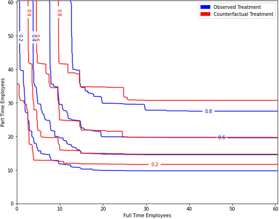
Postintervention quantile curves for observed treatment group units and their counterfactuals.

References

[1] Abadie A. Semiparametric difference-in-differences estimators. Rev Econ Stud. 2005;72(1):1–19. 10.1111/0034-6527.00321Search in Google Scholar
[2] Lechner M. The estimation of causal effects by difference-in-difference methods. Foundations and Trends® in Econometrics. 2011;4(3):165–224. 10.1561/0800000014Search in Google Scholar
[3] Imbens GW, Rubin DB. Causal inference in statistics, social, and biomedical sciences. New York, NY: Cambridge University Press; 2015. 10.1017/CBO9781139025751Search in Google Scholar
[4] Roth J, Sant’Anna PH, Bilinski A, Poe J. What’s trending in difference-in-differences? A synthesis of the recent econometrics literature. 2022. arXiv: http://arXiv.org/abs/arXiv:220101194. Search in Google Scholar
[5] Wing C, Simon K, Bello-Gomez RA. Designing difference in difference studies: best practices for public health policy research. Annual Review Public Health. 2018;39:453–69.10.1146/annurev-publhealth-040617-013507Search in Google Scholar PubMed
[6] Athey S, Imbens GW. Identification and inference in nonlinear difference-in-differences models. Econometrica. 2006;74(2):431–97. 10.1111/j.1468-0262.2006.00668.xSearch in Google Scholar
[7] Heckman J. Varieties of selection bias. Amer Econ Rev. 1990;80(2):313–8. Search in Google Scholar
[8] Roth J, Sant’Anna PH. When is parallel trends sensitive to functional form? 2020. arXiv: http://arXiv.org/abs/201004814. Search in Google Scholar
[9] Ryan AM, Kontopantelis E, Linden A, Burgess Jr JF. Now trending: Coping with non-parallel trends in difference-in-differences analysis. Stat Methods Med Res. 2019;28(12):3697–711. 10.1177/0962280218814570Search in Google Scholar PubMed
[10] Goodman-Bacon A, Marcus J. Using difference-in-differences to identify causal effects of COVID-19 policies. Survey Res Methods. 2020;14(2):153–8. 10.2139/ssrn.3603970Search in Google Scholar
[11] Drysdale KM, Hendricks NP. Adaptation to an irrigation water restriction imposed through local governance. J Environ Econ Management. 2018;91:150–65. 10.1016/j.jeem.2018.08.002Search in Google Scholar
[12] Peyré G, Cuturi M. Computational optimal transport. Foundations and Trends® in Machine Learning. 2019;11(5–6):355–607. 10.1561/2200000073Search in Google Scholar
[13] Card D, Krueger AB. Minimum wages and employment: a case study of the fast-food industry in New Jersey and Pennsylvania. Amer Econ Rev. 1994;84(4):772–93. 10.3386/w4509Search in Google Scholar
[14] Ghanem D, Sant’Anna PHC, Wüthrich K. Selection and parallel trends. 2022. arXiv: http://arXiv.org/abs/220309001. Search in Google Scholar
[15] Marx P, Tamer E, Tang X. Parallel trends and dynamic choices. 2022. arXiv: http://arXiv.org/abs/220706564. Search in Google Scholar
[16] Rigollet P, Weed J. Uncoupled isotonic regression via minimum Wasserstein deconvolution. Inform Inference A J IMA. 2019;8(4):691–717. 10.1093/imaiai/iaz006Search in Google Scholar
[17] Balabdaoui F, Doss CR, Durot C. Unlinked monotone regression. 2021. arXiv: http://arXiv.org/abs/arXiv:200700830. Search in Google Scholar
[18] Slawski M, Sen B. Permuted and unlinked monotone regression in Rd: an approach based on mixture modeling and optimal transport. 2022. arXiv: http://arXiv.org/abs/arXiv:220103528. Search in Google Scholar
[19] Callaway B, Li T. Quantile treatment effects in difference in differences models with panel data. Quantitative Econom. 2019;10(4):1579–618. 10.3982/QE935Search in Google Scholar
[20] Bonhomme S, Sauder U. Recovering distributions in difference-in-differences models: A comparison of selective and comprehensive schooling. Review Econom Stat. 2011;93(2):479–94. 10.1162/REST_a_00164Search in Google Scholar
[21] Brenier Y. Polar factorization and monotone rearrangement of vector-valued functions. Commun Pure Appl Math. 1991;44(4):375–417. 10.1002/cpa.3160440402Search in Google Scholar
[22] Caffarelli LA. Monotonicity properties of optimal transportation and the FKG and related inequalities. Comm Math Phys. 2000;214(3):547–63. 10.1007/s002200000257Search in Google Scholar
[23] Rockafellar RT. Convex analysis. Princeton, NJ: Princeton University Press; 1997. Search in Google Scholar
[24] Matzkin RL. Nonparametric estimation of nonadditive random functions. Econometrica. 2003;71(5):1339–75. 10.1111/1468-0262.00452Search in Google Scholar
[25] Chernozhukov V, Hansen C. An IV model of quantile treatment effects. Econometrica. 2005;73(1):245–61. 10.1111/j.1468-0262.2005.00570.xSearch in Google Scholar
[26] Imbens GW. Nonadditive models with endogenous regressors. Econometric Soc Monographs. 2007;43:17. 10.1017/CCOL0521871549.002Search in Google Scholar
[27] Ekeland I, Galichon A, Henry M. Comonotonic measures of multivariate risks. Math Finance. 2010 Oct;22(1):109–32. Search in Google Scholar
[28] Boissard E, Le Gouic T, Loubes JM. Distributionas template estimate with Wasserstein metrics. Bernoulli. 2015;21(2):740–59. 10.3150/13-BEJ585Search in Google Scholar
[29] Puccetti G, Scarsini M. Multivariate comonotonicity. J Multivariate Anal. 2010;101(1):291–304. 10.1016/j.jmva.2009.08.003Search in Google Scholar
[30] Ashlagi I, Braverman M, Hassidim A, Monderer D. Monotonicity and implementability. Econometrica. 2010;78(5):1749–72. 10.3982/ECTA8882Search in Google Scholar
[31] Rochet JC. A necessary and sufficient condition for rationalizability in a quasi-linear context. J Math Econom. 1987;16(2):191–200. 10.1016/0304-4068(87)90007-3Search in Google Scholar
[32] Shi X, Shum M, Song W. Estimating semi-parametric panel multinomial choice models using cyclic monotonicity. Econometrica. 2018;86(2):737–61. 10.3982/ECTA14115Search in Google Scholar
[33] Chernozhukov V, Galichon A, Henry M, Pass B. Identification of Hedonic equilibrium and nonseparable simultaneous equations. Journal of Political Economy. 2021;129(3):842–70. 10.1086/712447Search in Google Scholar
[34] Rüschendorf L. On c-optimal random variables. Stat Probability Lett. 1996;27(3):267–70. 10.1016/0167-7152(95)00078-XSearch in Google Scholar
[35] Gunsilius FF. A condition for the identification of multivariate models with binary instruments. J Econometrics. 2022;235:220–38. 10.1016/j.jeconom.2022.04.003Search in Google Scholar
[36] Galichon A. A survey of some recent applications of optimal transport methods to econometrics. Econometrics J. 2017;20(2):C1–11. 10.1111/ectj.12083Search in Google Scholar
[37] McCann RJ, Pass B. Optimal transportation between unequal dimensions. Archive Rational Mechanics Anal. 2020;238(3):1475–520. 10.1007/s00205-020-01569-5Search in Google Scholar
[38] Auricchio G, Veneroni M. On the structure of optimal transportation plans between discrete measures. Appl Math Optimiz. 2022;85(3):42. 10.1007/s00245-022-09861-4Search in Google Scholar
[39] Decancq K, Lugo MA. Weights in multidimensional indices of wellbeing: an overview. Econometric Rev. 2013;32(1):7–34. 10.1080/07474938.2012.690641Search in Google Scholar
[40] Duclos JY, Sahn DE, Younger SD. Robust multidimensional poverty comparisons. The Economic J. 2006;116(514):943–68. 10.1111/j.1468-0297.2006.01118.xSearch in Google Scholar
[41] Bourguignon F, Chakravarty SR. The measurement of multidimensional poverty. J Economic Inequality. 2003;1:25–49. 10.1023/A:1023913831342Search in Google Scholar
[42] Ekeland I, Galichon A, Henry M. Comonotonic measures of multivariate risks. Math Finance Int J Math Stat Financial Econom. 2012;22(1):109–32. 10.1111/j.1467-9965.2010.00453.xSearch in Google Scholar
[43] Embrechts P, McNeil A, Straumann D. Correlation and dependence in risk management: properties and pitfalls. Risk Management Value Risk Beyond. 2002;1:176–223. 10.1017/CBO9780511615337.008Search in Google Scholar
[44] Hallin M. Measure transportation and statistical decision theory. Ann Rev Stat Appl. 2022;9:401–24. 10.1146/annurev-statistics-040220-105948Search in Google Scholar
[45] García-Gómez C, Perez A, Prieto-Alaiz M. A review of stochastic dominance methods for poverty analysis. J Economic Surveys. 2019;33(5):1437–62. 10.1111/joes.12334Search in Google Scholar
[46] Embrechts P, Puccetti G. Bounds for functions of multivariate risks. J Multivariate Anal. 2006;97(2):526–47. 10.1016/j.jmva.2005.04.001Search in Google Scholar
[47] Shannon CE. A mathematical theory of communication. Bell Syst Technical J. 1948;27(3):379–423. 10.1002/j.1538-7305.1948.tb01338.xSearch in Google Scholar
[48] Forrow A, Hütter JC, Nitzan M, Rigollet P, Schiebinger G, Weed J. Statistical optimal transport via factored couplings. In: The 22nd International Conference on Artificial Intelligence and Statistics. PMLR; 2019. p. 2454–65. Search in Google Scholar
[49] Gunsilius FF. On the convergence rate of potentials of Brenier maps. Econometric Theory. Cambridge, England: Cambridge University Press; 2021. 10.1017/S0266466621000037Search in Google Scholar
[50] Hütter JC, Rigollet P. Minimax estimation of smooth optimal transport maps. Ann Stat. 2021;49(2):1166–94. 10.1214/20-AOS1997Search in Google Scholar
[51] de Lara L, González-Sanz A, Loubes JM. A consistent extension of discrete optimal transport maps for machine learning applications. 2021. arXiv: http://arXiv.org/abs/210208644. Search in Google Scholar
[52] Manole T, Balakrishnan S, Niles-Weed J, Wasserman L. Plugin estimation of smooth optimal transport maps. 2021. arXiv: http://arXiv.org/abs/arXiv:210712364. Search in Google Scholar
[53] Manole T, Niles-Weed J. Sharp convergence rates for empirical optimal transport with smooth costs. 2021. arXiv: http://arXiv.org/abs/arXiv:210613181. Search in Google Scholar
[54] Pooladian AA, Niles-Weed J. Entropic estimation of optimal transport maps. 2021. arXiv: http://arXiv.org/abs/arXiv:210912004. Search in Google Scholar
[55] Vacher A, Muzellec B, Rudi A, Bach F, Vialard FX. A dimension-free computational upper-bound for smooth optimal transport estimation. In: Proceedings of Thirty Fourth Conference on Learning Theory. PMLR; 2021. p. 4143–73. Search in Google Scholar
[56] Muzellec B, Vacher A, Bach F, Vialard FX, Rudi A. Near-optimal estimation of smooth transport maps with kernel sums-of-squares. 2021. arXiv: http://arXiv.org/abs/arXiv:211201907. Search in Google Scholar
[57] Deb N, Ghosal P, Sen B. Rates of estimation of optimal transport maps using plug-in estimators via barycentric projections. 2021. arXiv: http://arXiv.org/abs/arXiv:210701718. Search in Google Scholar
[58] Politis DN, Romano JP, Wolf M. On the asymptotic theory of subsampling. Stat Sinica. 2001;11:1105–24. Search in Google Scholar
[59] Romano JP, Shaikh AM. On the uniform asymptotic validity of subsampling and the bootstrap. Ann Stat. 2012;40(6):2798–822. 10.1214/12-AOS1051Search in Google Scholar
[60] Shao X, Politis DN. Fixed b subsampling and the block bootstrap: improved confidence sets based on p-value calibration. J R Stat Soc Ser B (Stat Methodol). 2013;75(1):161–84. 10.1111/j.1467-9868.2012.01037.xSearch in Google Scholar
[61] Neumark D, Wascher W. Minimum wages and employment: a case study of the fast-food industry in new jersey and pennsylvania: comment. Amer Econ Rev. 2000;90(5):1362–96. 10.1257/aer.90.5.1362Search in Google Scholar
[62] Dube A, Lester TW, Reich M. Minimum wage effects across state borders: Estimates using contiguous counties. Review Econom Stat. 2010;92(4):945–64. 10.1162/REST_a_00039Search in Google Scholar
[63] Meer J, West J. Effects of the minimum wage on employment dynamics. J Human Resources. 2016;51(2):500–22. 10.3368/jhr.51.2.0414-6298R1Search in Google Scholar
[64] Neumark D, Salas JI, Wascher W. Revisiting the minimum wage-Employment debate: Throwing out the baby with the bathwater? ILR Review. 2014;67(3 suppl):608–48. 10.1177/00197939140670S307Search in Google Scholar
[65] Lu B, Rosenbaum PR. Optimal pair matching with two control groups. J Comput Graph Stat. 2004;13(2):422–34. 10.1198/1061860043470Search in Google Scholar
[66] Ehrenberg RG, Brown C, Freeman RB, Hamermesh DS, Osterman P, Welch F. Myth and measurement: the new economics of the minimum wage. Industrial Labor Relations Review. 1995;48(4):827. 10.2307/2524359Search in Google Scholar
[67] Ropponen O. Reconciling the evidence of Card and Krueger (1994) and Neumark and Wascher (2000). J Appl Econometrics. 2011;26(6):1051–7. 10.1002/jae.1258Search in Google Scholar
[68] Segers J. Graphical and uniform consistency of estimated optimal transport plans. 2022. arXiv: http://arXiv.org/abs/arXiv:220802508. Search in Google Scholar
[69] Varadarajan VS. Weak convergence of measures on separable metric spaces. Sankhy Indian J Stat. 1958;19:15–22. Search in Google Scholar
[70] Rockafellar R. Characterization of the subdifferentials of convex functions. Pacific J Math. 1966;17(3):497–510. 10.2140/pjm.1966.17.497Search in Google Scholar
[71] Shorack GR, Wellner JA. Empirical processes with applications to statistics. Classics in Applied Mathematics. Philadelphia, PA: Society for Industrial and Applied Mathematics; 2009. 10.1137/1.9780898719017Search in Google Scholar
[72] Vapnik VN, Chervonenkis AY. On the uniform convergence of relative frequencies of events to their probabilities. Theory Probability Appl. 1971;16(2):264–80. 10.1137/1116025Search in Google Scholar
[73] Fournier N, Guillin A. On the rate of convergence in Wasserstein distance of the empirical measure. Probability Theory Related Fields. 2015;162(3):707–38. 10.1007/s00440-014-0583-7Search in Google Scholar
[74] Canas G, Rosasco L. Learning probability measures with respect to optimal transport metrics. In: Pereira F, Burges CJ, Bottou L, Weinberger KQ, editors. Advances in Neural Information Processing Systems. vol. 25. Boston, MA: Curran Associates, Inc.; 2012. https://proceedings.neurips.cc/paper/2012/file/c54e7837e0cd0ced286cb5995327d1ab-Paper.pdf. Search in Google Scholar
[75] Abadie A, Imbens GW. Large sample properties of matching estimators for average treatment effects. Econometrica. 2006 Jan;74(1):235–67. 10.1111/j.1468-0262.2006.00655.xSearch in Google Scholar
[76] Cuturi M. Sinkhorn distances: lightspeed computation of optimal transport. In: Advances in neural information processing systems. vol. 26. Boston, MA: Curran Associates, Inc.; 2013. Search in Google Scholar
[77] Altschuler J, Weed J, Rigollet P. Near-linear time approximation algorithms for optimal transport via Sinkhorn iteration. 2017. arXiv: http://arXiv.org/abs/170509634. Search in Google Scholar
[78] Papadakis N. Optimal transport for image processing [Habilitation à diriger des recherches]. Université de Bordeaux; Habilitation thesis; 2015. https://hal.science/tel-01246096. Search in Google Scholar
[79] Seguy V, Damodaran BB, Flamary R, Courty N, Rolet A, Blondel M. Large-scale optimal transport and mapping estimation. 2018. arXiv: http://arXiv.org/abs/171102283. Search in Google Scholar
[80] Makkuva AV, Taghvaei A, Oh S, Lee JD. Optimal transport mapping via input convex neural networks. 2020. arXiv: http://arXiv.org/abs/190810962. Search in Google Scholar
[81] Lu Y, Lu J. A Universal Approximation theorem of deep neural networks for expressing probability distributions. 2020. arXiv: http://arXiv.org/abs/200408867. Search in Google Scholar
[82] Flamary R, Courty N, Gramfort A, Alaya MZ, Boisbunon A, Chambon S, et al. POT: python optimal transport. J Machine Learn Res. 2021;22(78):1–8. Search in Google Scholar
© 2024 the author(s), published by De Gruyter
This work is licensed under the Creative Commons Attribution 4.0 International License.
Articles in the same Issue
- Research Articles
- Evaluating Boolean relationships in Configurational Comparative Methods
- Doubly weighted M-estimation for nonrandom assignment and missing outcomes
- Regression(s) discontinuity: Using bootstrap aggregation to yield estimates of RD treatment effects
- Energy balancing of covariate distributions
- A phenomenological account for causality in terms of elementary actions
- Nonparametric estimation of conditional incremental effects
- Conditional generative adversarial networks for individualized causal mediation analysis
- Mediation analyses for the effect of antibodies in vaccination
- Sharp bounds for causal effects based on Ding and VanderWeele's sensitivity parameters
- Detecting treatment interference under K-nearest-neighbors interference
- Bias formulas for violations of proximal identification assumptions in a linear structural equation model
- Current philosophical perspectives on drug approval in the real world
- Foundations of causal discovery on groups of variables
- Improved sensitivity bounds for mediation under unmeasured mediator–outcome confounding
- Potential outcomes and decision-theoretic foundations for statistical causality: Response to Richardson and Robins
- Quantifying the quality of configurational causal models
- Design-based RCT estimators and central limit theorems for baseline subgroup and related analyses