Quantifying the quality of configurational causal models

3.1 State-of-the-art in CCM benchmarking

Even though the output of a CCM inferred from limitedly diverse data often contains more than one model and even though these models cannot be expected to reflect the complete ground truth, the output as a whole can and should be expected to truthfully reflect the data-generating structure. This is satisfied if at least one output model m i is a submodel of the model representing the complete ground truth. Against that backdrop, the following is a qualitative correctness criterion frequently used in CCM benchmarking (e.g., [7,8,10,11,15,16]):^[7]

Qualitative correctness (LCR). A model m is a correct representation of a ground truth Δ iff m is a submodel of Δ .

While being important in current CCM benchmarking, (LCR) is clearly insufficient to assess the overall quality of models. For one, (LCR) does not take model complexity or informativeness into account. Models can be very sparse or very complex submodels of the ground truth, yet equally satisfy (LCR). Hence, correctness needs to be complemented by a completeness criterion suitably rewarding informativeness.^[8] There are various completeness criteria on offer, some qualitative [7], some quantitative [9,10,15,16], but they all measure completeness by drawing on the submodel relation.

Another reason why (LCR) does not suffice for assessing model quality is that it is merely qualitative, meaning it can only be passed or not. As a result, (LCR) cannot capture important differences. To illustrate, let Δ 1 be the ground truth and let models (4) and (5) be inferred from data simulated from that ground truth in a benchmark test:

As neither (4) nor (5) are submodels of Δ 1 , they are both incorrect according to (LCR). But there is a clear sense in which (4) is not equally incorrect as (5). While (4) correctly entails that A and D are causally relevant and places these causes in alternative disjuncts, it erroneously ascribes causal relevance to B (instead of b ). (5) makes that same mistake and, in addition, erroneously combines D conjunctively with A . That is, (5) commits one error more than (4). It should count as a worse representation of Δ 1 than (4). However, (LCR), being a mere qualitative criterion, is insensitive to such differences in number of errors.

To date, Arel-Bundock [9] is the only one who has proposed a measure that is sensitive to such differences by expressing correctness quantitatively. Strictly speaking, Arel-Bundock does not define a measure for model correctness but for model wrongness: “I measure the level of wrongness by counting the proportion of solution submodels that are not submodels of the truth” [9, p. 7]. But to adjust this proposal to our preferred terminology (which is also standard in the benchmarking literature), we transform Arel-Bundock’s wrongness measure into a quantitative correctness measure (by negating it):

Quantitative correctness (NCR). The correctness of a model m for a ground truth Δ is the proportion of m ’s submodels that are also submodels of Δ .

To illustrate, we apply (NCR) to models (4) and (5). Table 1 lists all submodels of (4) and (5), respectively, and indicates whether they are submodels of the ground truth Δ 1 . Three of the seven submodels of (4) are also submodels of Δ 1 , yielding a (NCR)-score of 0.43. With only two of its seven submodels being submodels of Δ 1 , (5) gets a (NCR)-score of 0.29. That these scores are below 1 and above 0 reflects the fact that neither (4) nor (5) are fully correct representations of Δ 1 while still making some true claims. Furthermore, (4) receives a higher score than (5) because it makes less errors. On the face of it, (NCR) thus seems to capture exactly those differences that (LCR) is insensitive to. However, the next two sections will show that (NCR) does not adequately score model correctness in all cases.

3.2 Problem of overcounting errors

The first problem of (NCR) is best introduced with another concrete example. Thus, let Δ 2 be the ground truth and let models (6)–(8) be inferred from data simulated from Δ 2 :

The important feature of candidate models (6)–(8) is that they all contain the same error: instead of adding D to the first or second disjunct, they place D into a third disjunct, thus, claiming that D brings about E independently of the other factors. Apart from that mistake, all other causal claims entailed by (6)–(8) are true of Δ 2 . More specifically, the difference between (6) and (7) is that the latter truthfully identifies A ∗ b as a cause of E , while in the former b is not part of the first disjunct. That is, (7) makes the same mistake as (6) and contains more true information. Analogously, (8) features the same error as (7) (and (6)) in combination with the true conjunctive addition of F to A ∗ b .

Clearly, an adequate correctness measure must not punish models (7) and (8) for containing more true elements than (6) while committing the same error as (6). More generally, an adequate correctness measure should respect the following model expansion principle (MEP):

Model Expansion Principle (MEP). Expanding a model by truthfully located elements from the ground truth cannot reduce correctness.

(NCR), however, does not respect (MEP). It assigns the highest correctness score to (6) and the lowest to (8). Model (6) has a total of seven submodels, six of which are also submodels of Δ 2 , yielding an (NCR)-score of 6 ∕ 7 = 0.86 , whereas (7) and (8) only reach (NCR)-scores of 12 ∕ 15 = 0.80 and 24 ∕ 31 = 0.77 , respectively.^[9] The reason for this inadequate scoring, in a nutshell, is that (NCR) counts both true and false claims made by models multiple times, in a possibly disproportional manner, which leads to an overcounting of false claims, i.e., of errors in case of models (7) and (8).

To bring this out more clearly, we take a closer look at (7). Table 2 lists all of (7)’s 15 submodels. The truthful submodels, i.e., the ones that are submodels of Δ 2 , are in the left half of the table, the false ones in the right. For each submodel, the table indicates whether it is also a submodel of (6). The first thing to highlight is the tendency of (NCR) to count false and true claims made by (7) and its submodels multiple times. For instance, according to Δ 2 , it is false to say, as does sm 15 , that C and D are parts of alternative causes of E , rather they are causally relevant in conjunction. This entails that submodels sm 13 and sm 14 are also false, as they result from sm 15 by mere elimination of a conjunct. The error contained in sm 13 and sm 14 is the same as the error in sm 15 . Analogously, given that sm 11 is a submodel of Δ 2 , and thus only makes true causal claims, it follows that all submodels of sm 11 , as sm 7 to sm 9 , are also submodels of Δ 2 , and thus true of Δ 2 . That is, models sm 7 to sm 9 do not reveal any truths about Δ 2 not revealed by sm 11 . Although many submodels of (7) commit the same errors or reveal the same truths, (NCR) counts all of them separately in its correctness calculation.

Now, observe what proportions of true and false submodels are added when model (6) is expanded to (7). Model (6) has seven submodels, which are also marked in Table 2. Six of these submodels are true, one is false. When b is truthfully integrated into (6) to yield model (7), six true and two false submodels are added to the count. That is, the proportion of false submodels increases by a factor of 3 ∕ 1 = 3 , whereas the proportion of true submodels only multiplies by 12 ∕ 6 = 2 . In other words, even though (7) results from (6) by integrating true elements only, disproportionally more false than true submodels are thereby introduced. The same happens when (7) is further expanded to (8). It follows that measuring correctness in terms of proportions of true submodels, as done by (NCR), cannot possibly do justice to (MEP).

We take this to show that not only (NCR) does not adequately quantify model correctness but any attempt to quantify correctness based on proportions of true or false submodels faces a risk of miscounting errors, because those proportions can be twisted under model expansion and thus are not guaranteed to respect (MEP).

3.3 Problem of indirect causation

To date, CCM benchmarking has predominantly focused on QCA’s or CNA’s success in recovering single-outcome models, i.e., atomic MINUS-formulas. Correspondingly, both (LCR) and (NCR) are custom-built for correctness assessment in single-outcome recovery. This section argues that (LCR) and (NCR) are in fact inadequate when the data are generated by multi-outcome structures with causally related outcomes, i.e., by causal chains. In a nutshell, the reason is that models leaving out intermediate links on causal paths to an ultimate outcome may be perfectly correct without being a submodel of the ground truth or even containing such a submodel.

To see this, consider the causal chains in the hypergraph of Figure 1. This graph has two non-standard elements that require introduction: arrows merged by “•” symbolize conjunctive relevance, and “◇” expresses that the negation of the factor at the tail of the arrow is relevant. Another notable feature of that structure, which will become important in Section 4.1, is the switching factor F: its positive value F determines that the impact of B on G is transmitted via D and its negative value f causes that impact to be mediated by E (for more details see [2]). The complex MINUS-formula in Δ 3 expresses that switching structure. Let us assume that Δ 3 is the ground truth used to simulate data in some benchmark test in which the examined method returns model (9). When causally interpreted, (9) claims that A and B are causally relevant for G and that they are parts of alternative causes producing G independently of one another. Both of these claims are indeed true of Δ 3 , according to which A and B are alternative causes of D and D is a cause of G , making A and B indirect alternative causes of G . Model (9) is just incomplete. It leaves out the middle link mediating the causal influence of A and B to G – as well as numerous other causes of G . But, as we have seen before, incompleteness does not make a model incorrect.

Figure 1

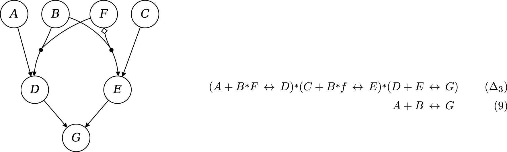
A causal chain with switching factor F, the corresponding complex MINUS-formula Δ 3 , and a candidate model (9). Arrows merged by “•” symbolize conjunctive relevance and “◇” expresses that the negation of the factor at the tail of the arrow is relevant.

One might be inclined to respond that, despite making numerous true claims about Δ 3 , (9) also falsely claims that A and B are direct causes of G , where in truth they are indirect causes. This response presupposes that there is an objective fact of the matter as to whether a cause – in truth – directly or indirectly brings about its effect. In light of the (widely assumed) continuity of spacetime, however, it is possible to interpolate (suitably defined) intermediate factors on virtually any causal path between two factors. Only extremely fine-grained models representing causal structures on the level of objectively fundamental particles – if such exist at all – , could conceivably trace direct causation. Such a view would entail that all macro-level models are incorrect (to some degree) because they represent causal dependencies as direct, which in fact are mediated by intermediate links.

To avoid that consequence, it is standard to view the distinction between direct and indirect causation as inherently relative to the factors contained in a given model [26,27]. That means that a causal relation can be truthfully represented as a direct one in a first model and as an indirect one in a second. Relative to the factors in model (9), A and B are indeed direct causes of G , because D and E are not contained in (9). But as D and E are contained in Δ 3 , the relevance of A and B for G becomes mediated and thus indirect. But Δ 3 might likewise be expandable by further intermediate links, whereby relations represented as direct ones in Δ 3 would be turned into indirect ones. There is no need to stipulate that Δ 3 is an objectively fundamental representation of a causal structure; rather, it truthfully depicts a segment of reality relative to a set of factors suited for that purpose. But the same segment might also be truthfully represented on another level of granularity using other factors.^[10]

Against that backdrop, model (9) is incomplete but does not commit an error. An adequate correctness measure should thus reward it with a maximal score. However, both (LCR) and (NCR) fail to do so. The only atomic MINUS-formula for outcome G (i.e., the outcome of (9)) contained in Δ 3 is this one:

But (9) is neither itself a submodel of (10), and thereby of Δ 3 , nor does it contain a submodel that would be a submodel of (10), i.e., of Δ 3 . It follows that (9) does not pass (LCR) and that it receives an (NCR)-score of 0 ∕ 3 = 0 .

4.1 Building causal expositions

MINUS-formulas contain four types of causal information: ascriptions of causal relevance (i) to individual factor values (or literals), (ii) to conjunctions, (iii) to disjunctions, and (iv) sequential orderings of causal relations in causal paths. For brevity, we refer to these types as literal, conjunctive, disjunctive, and sequential ascriptions, respectively. To illustrate, reconsider Δ 3 , which represents the switching structure in Figure 1:

Among many others, Δ 3 makes the literal ascription that A is causally relevant to G , the conjunctive ascription that B ∗ F is relevant to D , the disjunctive ascription that D + E is relevant to G , or the sequential ascription that there exists a causal path from A via D to G , expressible as ordered sequence ⟨ A , D , G ⟩ . We call the compilation of all causal information contained in a MINUS-formula its causal exposition:

Causal exposition. The causal exposition of a MINUS-formula m is the list of all literal, conjunctive, disjunctive, and sequential ascriptions entailed by m .

One lesson to learn from the problem of indirect causation is that causal expositions cannot simply be read off the syntax of a MINUS-formula (or of its submodels), because MINUS-formulas only represent direct causation (relative to the factors in the formula) and lack a syntactic expression of indirect causation. But information about indirect causation, and thus causal expositions, can be recovered from MINUS-formulas by syntactic transformations standard in Boolean algebra.

Viewed as a mere Boolean expression, the first atomic MINUS-formula in Δ 3 , viz. A + B ∗ F ↔ D , states that A + B ∗ F and D are equivalent, which entails that they are substitutable for one another without breach of Boolean dependence relations of sufficiency and necessity. This substitutability principle allows for replacing D in the third atomic formula in Δ 3 , viz. in D + E ↔ G , by A + B ∗ F .

(11) is automatically in DNF. In other examples, additional transformations – for instance, factoring out – may be required to bring expressions resulting from such substitutions into DNF; but any Boolean expression can easily be brought into DNF. The substitutability principle ensures that if D + E ↔ G truthfully expresses Boolean dependence relations, then so does (11). But the principle does not guarantee that the expression resulting from the substitution remains redundancy-free and thus causally interpretable. And indeed, (11) contains a redundancy: in the set of all configurations compatible with Δ 3 , i.e., in so-called ideal data (i.e., noise-free and unfragmented data) generated from Δ 3 , F does not make a difference to G . The factor F is a mere switch in Δ 3 ; its positive value F determines that the causal impact of B is transmitted via D to G and its negative value f causes that impact to be mediated by E ; but whichever value F takes, B itself is sufficient for G .^[11] Hence, B ∗ F in (11) is only sufficient for G but not minimally so.

If we additionally minimize sufficient and necessary conditions in (11) relative to ideal data on Δ 3 (e.g., by means of Quine–McCluskey optimization [28]), we obtain this expression:

(12) has the form of an atomic MINUS-formula. As it results from syntactic transformations of Δ 3 , it can be seen as representing relations of indirect causation entailed by Δ 3 . It states that A and B are causally relevant for G , which, relative to the set of factors in Δ 3 , amounts to indirect relevance. For brevity, we call it an indirect MINUS-formula relative to Δ 3 . Indirect MINUS-formulas are recoverable from complex MINUS-formulas by substitution of equivalents, DNF transformation, if needed, and Boolean minimization.

Two further indirect MINUS-formulas can be recovered from Δ 3 in the same way. (13) is built by substituting C + B ∗ f for E in D + E ↔ G , and (14) is the result of replacing both D and E by their equivalents in Δ 3 and subsequent minimization:

(12), (13), and (14) are all the indirect MINUS-formulas recoverable from Δ 3 . We will call the union of all atomic (direct) MINUS-formulas in Δ 3 and all indirect MINUS-formulas recoverable from it the chain-expansion of Δ 3 . But before we can explicitly define that notion, we have to consider the case where the complex MINUS-formula to be chain-expanded is not a ground truth but a model inferred from data.

Hence, suppose that the following multi-outcome model is inferred from data simulated from ground truth Δ 3 :

If we substitute D in D + E ↔ G by its equivalent A + B ∗ F and then minimize relative to ideal data on (15), we do not end up with (12) but with (11). That is, if indirect MINUS-formulas are recovered from (15) through Boolean minimization relative to ideal data on (15), F appears to make a difference to G because F is no switching factor in (15). However, (15) is not inferred from ideal data generated from itself but from data simulated from Δ 3 , and according to Δ 3 , F does not make a difference to G . That means that the data from which (15) is inferred do not contain evidence for the indirect relevance of F for E . It would therefore not be adequate to recover an indirect relevance ascription from (15) for which there is no evidential basis in the discovery context of that model. We thus submit that when indirect causation is recovered from models inferred from data, Boolean minimization should be conducted relative to that actual data and not, as in case of chain-expanding ground truths, relative to ideal data. In sum, the following is our definition of the notion of a chain-expansion:

Chain-expansion. The chain-expansion of a MINUS-formula m is the union of the atomic (direct) MINUS-formulas contained in m and the indirect MINUS-formulas recoverable from m by substitution of equivalents, DNF transformation, and Boolean minimization, either relative to the data from which m is inferred or, if m is not inferred from data, relative to ideal data on m .

The important feature of chain-expansions for quantifying model quality is that they syntactically represent all types of causal ascriptions entailed by a MINUS-formula m . The literal, conjunctive, and disjunctive ascriptions of m for an outcome Z are simply the sets of all factor values and all maximally long conjunctions and disjunctions – freed of duplicates – that appear on the left-hand side of “ ↔ ” in the atomic MINUS-formulas for Z in m ’s chain-expansion. The sequential ascriptions for outcome Z are the maximally long ordered sequences of factor values ⟨ X 1 , … , X n ⟩ satisfying the following path-rule: for all X i and X j with i < j in ⟨ X 1 , … , X n ⟩ , there is a MINUS-formula in m ’s chain-expansion with X i on the left-hand side and X j on the right-hand side of “ ↔ ”, and Z is the last element of the sequence (i.e., X n = Z ).

Table 3 lists the chain-expansion of Δ 3 in the left-most column and the causal exposition, subdivided by outcomes, in the other columns. The literal ascriptions for each outcome in Δ 3 can be recovered from the chain-expansion by removing conjunctors “ ∗ ”, disjunctors “ + ”, and duplicates from the expressions on the left-hand side of “ ↔ ”. The conjunctive ascriptions are obtained by removing “ + ” and duplicates, and the disjunctive ascriptions are simply the expressions on the left-hand side of “ ↔ ”. Note that, in case of outcome G , conjunctive ascriptions are identical to literal ones because none of G ’s MINUS-formulas actually features a conjunctor, and a single factor value formally counts as a trivial conjunction (and disjunction). Finally, sequential ascriptions are built by combining as many factor values as possible from the literal ascriptions following the path-rule for every outcome. In case of outcome G , this amounts to combining the factor values on the left-hand sides of D ’s and E ’s MINUS-formulas with D and E and adding G if, and only if, the first element of the sequence also appears on the left-hand side of a MINUS-formula of G .

4.2 Intersecting causal expositions

To quantify the correctness of a model m relative to a ground truth Δ , we propose to intersect the literal, conjunctive, disjunctive, and sequential ascriptions rendered transparent by the causal expositions of m and Δ . The ratios of the complexities of these intersections to the complexities of m ’s literal, conjunctive, disjunctive, and sequential ascriptions then yield measures for literal, conjunctive, disjunctive, and sequential correctness.

To make that concrete, assume that the following model is inferred from data generated by ground truth Δ 3 .

Model (16), which contains no information about outcome E , makes two false claims about Δ 3 : first, it erroneously places A and B in the same conjunctive cause of D , and second, B and C appear in the same conjunctive cause of G , which in truth are alternative indirect causes of G . But all literal ascriptions and the placement of D in a separate disjunct leading to G are true of Δ 3 . To quantify the correctness of (16), we first chain-expand that model by replacing D in the atomic MINUS-formula of G by A ∗ B and then build its causal exposition. The result is in Table 4.

Intersecting the literal, conjunctive, and disjunctive ascriptions of (16) and Δ 3 (cf. Table 3) for each outcome is straightforward. The literal intersection is the set of factor values contained in the literal ascriptions of both (16) and Δ 3 . The conjunctive intersection is the set of all conjunctions with a maximal amount of conjuncts that can be reached from the conjunctive ascriptions of both (16) and Δ 3 by mere elimination of conjuncts. For example, the (trivial) conjunction B can be reached from (16)’s conjunctive ascription A ∗ B for outcome D by elimination of A as well as from Δ 3 ’s conjunctive ascription B ∗ F for the same outcome by elimination of F , and there are no conjunctions reachable in that manner with more conjuncts, meaning that B has a maximal amount of conjuncts. The disjunctive intersection is the set of all disjunctions with a maximal amount of disjuncts that can be reached from the disjunctive ascriptions of both (16) and Δ 3 by elimination of disjuncts and conjuncts. For example, the disjunctive ascription D + B can be reached by elimination of C from (16)’s disjunctive ascription D + B ∗ C for outcome G as well as from Δ 3 ’s disjunctive ascription B + C + D for the same outcome, and there are no longer disjunctions reachable in that manner. Table 5 lists all intersections of (16) and Δ 3 . As can easily be seen from that table, conjunctive and disjunctive intersections tend to contain multiple elements; i.e., multiple conjunctions and disjunctions with maximal amounts of conjuncts and disjuncts can be reached from both (16) and Δ 3 .

As the difference between direct and indirect causal relevance is relative to a set of modeled factors, the correctness of the sequential ascriptions of a model must be assessed relative to its set of factors. This, in turn, requires that the sequential ascriptions of the corresponding ground truth be pruned to the model’s factor set before intersecting. More concretely, model (16) is correct to entail that B is a direct cause of G , despite B being an indirect cause of G in Δ 3 . The reason is that (16) does not feature the factor E , which is the intermediate link between B and G in Δ 3 , meaning that relative to the factors in (16) B indeed is a direct cause of G . Hence, before intersecting sequential ascriptions, factor E must be removed from the sequential ascriptions of Δ 3 , which is represented by “ E ” in Table 5. After such harmonizing, the sequential intersection of (16) and Δ 3 simply comes down to the set of sequential ascriptions made by both (16) and Δ 3 .

4.3 Quantifying correctness

An intersection expresses the amount of causal information of a particular type shared by the model and ground truth, in other words, it expresses the causal claims made by the model that are true of the ground truth, i.e., the model’s true positives. As correctness is a measure for the ratio of true information in a model, the next step toward putting a number on the correctness of (16), is to quantify the complexities of intersections and corresponding ascriptions. For literals, conjunctions, and disjunctions we quantify complexities in terms of numbers of factor values. For instance, the set { A , B } of (16)’s literal ascriptions for outcome D has complexity 2 because it contains two factor values; or the set { D + B ∗ C , A ∗ B + B ∗ C } of its disjunctive ascriptions for outcome G has complexity 7 because it contains seven factor values. The ratio of true information, then, is the ratio of factor values in these ascriptions that have counterparts in the corresponding intersections. Thus, since all factor values in { A , B } have counterparts in the literal intersection (see the first row of Table 5), the correctness ratio of { A , B } is 2 ∕ 2 . By contrast, the disjunctive ascriptions for outcome G are not completely represented in the disjunctive intersection (row 9 of Table 5). The first disjunction D + B ∗ C can be paired with either D + B or D + C in the corresponding intersection, and since both of the latter have equal complexity, it does not matter which of them is chosen as counterpart. The same holds for the second disjunction A ∗ B + B ∗ C : it can be paired with either A + B or A + C or B + C in the intersection. Whichever elements of the intersection are chosen as counterparts, a total of four of the seven factor values in the set of disjunctive ascriptions for outcome G have counterparts in the corresponding intersection, yielding a correctness ratio of 4 ∕ 7 . In Table 5, the factor values used for calculating the correctness ratios are highlighted in bold.

For sequences, we aim to avoid unnecessary double-counting by quantifying complexities not in terms of the number of factor values but in terms of the number of paths. That is, correctness ratios for the sequential ascriptions of a model are ratios of the model’s paths that are contained in the sequential intersection with the ground truth. For example, as both paths in the set of sequential ascriptions { ⟨ B , D ⟩ , ⟨ A , D ⟩ } for outcome D are also contained in the sequential intersection for that outcome, that set receives a correctness ratio of 2 ∕ 2 .

The next step to a correctness quantification of (16) consists in aggregating these correctness ratios of the component ascriptions. We choose a weighted mean for that purpose, where weights are the complexity shares of component ascriptions. For literal, conjunctive, and disjunctive correctness, weights are calculated based on the number of factor values in a corresponding ascription. In the case of sequential correctness, they are based on the number of paths. For instance, for both outcomes combined, the conjunctive ascriptions of (16) have a total complexity of seven factor values, with two pertaining to outcome D and five to outcome G . That is, the weights for the component ascriptions { A ∗ B } and { D , B ∗ C , A ∗ B } are 2 ∕ 7 and 5 ∕ 7 , respectively. Weighing the components’ ratios by these weights yields a conjunctive correctness score of 0.57. Or, the sequential ascription of (16) contains a total of six paths, with two leading to outcome D and four to outcome G , resulting in the weights 2 ∕ 6 and 4 ∕ 6 , respectively, and an overall sequential correctness score of 1. Table 5 provides an overview of all weights and resulting correctness scores.

Finally, the four correctness scores must be aggregated into one overall score, which we again do with a weighted mean. The weights are based on the complexity shares of a model’s whole causal exposition covered by a corresponding correctness score. The total complexity of the causal exposition is the sum of the complexities of the four types of causal ascriptions. For model (16), it is 6 + 7 + 9 + 6 = 28 , resulting in the weights indicated in the bottom row of Table 5. Overall, the correctness score of model (16) relative to ground truth Δ 3 is 0.75.

Here, then, is our quantitative correctness measure in condensed form. Let m be a CCM model inferred from data generated from a ground truth Δ . Let l O i ( m ) , c O i ( m ) , d O i ( m ) , and s O i ( m ) be m ’s literal, conjunctive, disjunctive, and sequential ascriptions for outcome O i , i = 1 , . . . , n , and analogously for l O i ( Δ ) , c O i ( Δ ) , d O i ( Δ ) , and s O i ( Δ ) . Moreover, let ∣ … ∣ denote the complexity of the enclosed expression, and let w O i x , x ∈ { l , c , d , s } , be the weight associated with the corresponding causal ascriptions of the i th outcome O i . Then, literal, conjunctive, disjunctive, and sequential correctness, ( Corr l ), ( Corr c ), ( Corr d ), and ( Corr s ) are defined as follows:

Aggregating these measures yields the following measure for overall correctness:

Correctness (Corr). The overall correctness of m for Δ is the weighted mean of m ’s ( Corr l ), ( Corr c ), ( Corr d ), and ( Corr s ) scores, or formally, where w x are the corresponding weights:

An isolated (Corr)-score as 0.75 for (16) is not very informative; it merely says that (16) is neither entirely correct nor entirely incorrect. How (in)correct it is becomes clear only if its correctness score is compared with the scores of other models inferred from the same data. Table 6a thus lists the (Corr)-scores of further model candidates assumed to be inferred from the same data simulated from Δ 3 as (16).^[12] The first model, m 1 , coincides with (16), except that it does not include D as cause of G . By leaving out D , m 1 leaves out a correct alternative cause of G . Contrary to (16), though, m 1 is not a chain, meaning that A ∗ B , to which (16) erroneously ascribes causal relevance for both D and G , is not entailed to be causally relevant for G by m 1 , which thereby avoids a false conjunctive ascription. Overall, m 1 receives the same (Corr)-score as (16). In model m 2 , the incorrect conjunction A ∗ B of (16) is replaced by a correct disjunction A + B ↔ D , and model m 3 even gets B + C ↔ G right. Correspondingly, the (Corr)-score of m 2 is higher than (16)’s and lower than m 3 ’s. As m 3 contains no error, it receives a perfect (Corr)-score. Likewise, m 4 , which was used to illustrate the problem of indirect causation in Section 3.3, is error-free and scores perfectly. The same holds for m 5 , because it is true that A and B are direct causes of G relative to the set { A , B , E , G } . That is not true for model m 6 , which additionally contains the link D mediating the causal impact of A and B on G in the ground truth Δ 3 . It follows that m 6 erroneously entails that A and B are direct causes of G and alternatives to D relative to the set { A , B , D , E , G } . Model m 6 reaches a disjunctive correctness of 0.75 and a sequential correctness of 0.5, which, with the perfect literal and conjunctive scores, aggregate to 0.81. Finally, while m 6 makes no incorrect literal and conjunctive ascriptions, m 7 , by falsely ascribing causal relevance for G to F , commits errors in all types of ascriptions. Correspondingly, its (Corr)-score is the lowest.

Finally, Table 6b exhibits the (Corr)-scores of the examples demonstrating the shortcomings of (NCR) in Section 3.2. Model (8) has the highest and (6) the lowest score. That is, contrary to (NCR), (Corr) does not punish (8) for containing more true information than (6), while committing the same mistake as (6). This result generalizes. Adding truthfully located elements from the ground truth to a model increases the complexities of the literal, conjunctive, disjunctive, and sequential intersections and of the model’s corresponding causal ascriptions by the same amount, meaning that numerators and denominators of ( Corr l ), ( Corr c ), ( Corr d ), and ( Corr s ) increase by the same amount as well. Hence, truthfully expanding models while keeping errors constant increases the (Corr)-score or keeps it constant. By contrast, adding errors to a model while keeping the true information constant only increases the complexities of a model’s causal ascriptions but not of their intersections with the ground truth’s causal ascriptions. In consequence, the numerators of ( Corr l ), ( Corr c ), ( Corr d ), and ( Corr s ) stay the same and the denominators increase, inducing the (Corr)-score to drop or to stay at the minimum of 0. In sum, (Corr) does neither overcount false nor true information in models. It does justice to the (MEP).

References

[1] Spirtes P, Glymour C, Scheines R. Causation, prediction, and search (second edition). Cambridge: MIT Press; 2000. 10.7551/mitpress/1754.001.0001Search in Google Scholar
[2] Baumgartner M, Falk C. Boolean difference-making: a modern regularity theory of causation. British J Philos Sci. 2023;74(1):171–97. 10.1093/bjps/axz047Search in Google Scholar
[3] Mackie JL. The cement of the universe: a study of causation. Oxford: Clarendon Press; 1974. Search in Google Scholar
[4] Ragin CC. The comparative method. Berkeley: University of California Press; 1987. Search in Google Scholar
[5] Rihoux B, Ragin CC (Ed.). Configurational comparative methods: Qualitative Comparative Analysis (QCA) and related techniques. Thousand Oaks: Sage; 2009. 10.4135/9781452226569Search in Google Scholar
[6] Baumgartner M. Uncovering deterministic causal structures: a Boolean approach. Synthese. 2009;170:71–96. 10.1007/s11229-008-9348-0Search in Google Scholar
[7] Baumgartner M, Ambühl M. Causal modeling with multi-value and fuzzy-set Coincidence Analysis. Politic Sci Res Methods. 2020;8(3):526–42. 10.1017/psrm.2018.45Search in Google Scholar
[8] Swiatczak MD. Different algorithms, different models. Quality Quantity. 2022;56:1913–37. 10.1007/s11135-021-01193-9Search in Google Scholar
[9] Arel-Bundock V. The double bind of Qualitative Comparative Analysis. Sociol Methods Res. 2022;51(3):963–82. 10.1177/0049124119882460Search in Google Scholar
[10] Baumgartner M, Falk C. Configurational causal modeling and logic regression. Multivariate Behav Res. 2023;58(2):292–310. 10.1080/00273171.2021.1971510Search in Google Scholar PubMed
[11] Baumgartner M, Thiem A. Often trusted but never (properly) tested: evaluating Qualitative Comparative Analysis. Sociol Methods Res. 2020;49(2):279–311. 10.1177/0049124117701487Search in Google Scholar
[12] Dusa A. Critical tension: sufficiency and parsimony in QCA. Sociol Methods Res. 2022 Nov;51(2):541–65. 10.1177/0049124119882456Search in Google Scholar
[13] Krogslund C, Choi DD, Poertner M. Fuzzy sets on shaky ground: parameter sensitivity and confirmation bias in fsQCA. Politic Anal. 2015;23(1):21–41. 10.1093/pan/mpu016Search in Google Scholar
[14] Lucas SR, Szatrowski A. Qualitative Comparative Analysis in critical perspective. Sociol Methodol. 2014;44(1):1–79. 10.1177/0081175014532763Search in Google Scholar
[15] Parkkinen VP, Baumgartner M. Robustness and model selection in configurational causal modeling. Sociol Methods Res. 2023;52(1):176–208. 10.1177/0049124120986200Search in Google Scholar
[16] Swiatczak MD, Baumgartner M. Data imbalances in Coincidence Analysis: a simulation study. Sociol Methods Res. 2024 March. DOI: https://doi.org/10.1177/00491241241227039. 10.1177/00491241241227039Search in Google Scholar
[17] Cheng L, Guo R, Moraffah R, Sheth P, Candan KS, Liu H. Evaluation methods and measures for causal learning algorithms. IEEE Trans Artif Intel. 2022;3(6):924–43. 10.1109/TAI.2022.3150264Search in Google Scholar
[18] Maier M, Taylor B, Oktay H, Jensen D. Learning causal models of relational domains. Proc AAAI Confer Artif Intell. 2010;24:531–8. DOI: https://doi.org/10.1609/aaai.v24i1.7695.10.1609/aaai.v24i1.7695Search in Google Scholar
[19] Meek C. Causal inference and causal explanation with background knowledge. In Proceedings of the Eleventh Conference on Uncertainty in Artificial Intelligence. 1995. p. 403–10. https://arxiv.org/ftp/arxiv/papers/1302/1302.4972.pdf. Search in Google Scholar
[20] Tabib Mahmoudi F, Samadzadegan F, Reinartz P. Object recognition based on the context aware decision level fusion in multi views imagery. IEEE J Selected Topics Appl Earth Observations Remote Sensing. 2015 Jan;8(1):12–22. 10.1109/JSTARS.2014.2362103Search in Google Scholar
[21] Beirlaen M, Leuridan B, Van De Putte F. A logic for the discovery of deterministic causal regularities. Synthese. 2018;195(1):367–99. 10.1007/s11229-016-1222-xSearch in Google Scholar
[22] Bowran AP. A Boolean algebra: abstract and concrete. London: Macmillan; 1965. 10.1007/978-1-349-00216-0Search in Google Scholar
[23] Lemmon EJ. Beginning logic. London: Chapman & Hall; 1965. Search in Google Scholar
[24] Ragin CC. Set relations in social research: evaluating their consistency and coverage. Political Analysis. 2006;14(3):291–310. 10.1093/pan/mpj019Search in Google Scholar
[25] Baumgartner M. Qualitative Comparative Analysis and robust sufficiency. Quality Quantity. 2022;56:1939–63. 10.1007/s11135-021-01157-zSearch in Google Scholar PubMed PubMed Central
[26] Parkkinen VP. Variable relativity of causation is good. Synthese. 2022;200:194. DOI: https://doi.org/10.1007/s11229-022-03676-0.10.1007/s11229-022-03676-0Search in Google Scholar
[27] Woodward J. Response to Strevens. Philosophy Phenomenol Res. 2008;LXXVII:193–212, 10.1111/j.1933-1592.2008.00181.xSearch in Google Scholar
[28] McCluskey EJ. Minimization of Boolean functions. Bell Syst Tech J. 1956;35:1417–44. 10.1002/j.1538-7305.1956.tb03835.xSearch in Google Scholar
[29] Haesebrouck T, Thomann E. Introduction: causation, inferences, and solution types in configurational comparative methods. Quality Quantity. 2022;56(4):1867–88. 10.1007/s11135-021-01209-4Search in Google Scholar
[30] Chinchor N. Muc-4 evaluation metrics. In Proceedings of the 4th Conference on Message Understanding. 1992 June. p. 22–29. https://aclanthology.org/M92-1002.pdf. 10.3115/1072064.1072067Search in Google Scholar
© 2024 the author(s), published by De Gruyter
This work is licensed under the Creative Commons Attribution 4.0 International License.
Articles in the same Issue
- Research Articles
- Evaluating Boolean relationships in Configurational Comparative Methods
- Doubly weighted M-estimation for nonrandom assignment and missing outcomes
- Regression(s) discontinuity: Using bootstrap aggregation to yield estimates of RD treatment effects
- Energy balancing of covariate distributions
- A phenomenological account for causality in terms of elementary actions
- Nonparametric estimation of conditional incremental effects
- Conditional generative adversarial networks for individualized causal mediation analysis
- Mediation analyses for the effect of antibodies in vaccination
- Sharp bounds for causal effects based on Ding and VanderWeele's sensitivity parameters
- Detecting treatment interference under K-nearest-neighbors interference
- Bias formulas for violations of proximal identification assumptions in a linear structural equation model
- Current philosophical perspectives on drug approval in the real world
- Foundations of causal discovery on groups of variables
- Improved sensitivity bounds for mediation under unmeasured mediator–outcome confounding
- Potential outcomes and decision-theoretic foundations for statistical causality: Response to Richardson and Robins