Nonparametric estimation of conditional incremental effects
-
Alec McClean
 ,
Zach Branson
,
Zach Branson

Abstract
Conditional effect estimation has great scientific and policy importance because interventions may impact subjects differently depending on their characteristics. Most research has focused on estimating the conditional average treatment effect (CATE). However, identification of the CATE requires that all subjects have a non-zero probability of receiving treatment, or positivity, which may be unrealistic in practice. Instead, we propose conditional effects based on incremental propensity score interventions, which are stochastic interventions where the odds of treatment are multiplied by some factor. These effects do not require positivity for identification and can be better suited for modeling scenarios in which people cannot be forced into treatment. We develop a projection approach and a flexible nonparametric estimator that can each estimate all the conditional effects we propose and derive model-agnostic error guarantees showing that both estimators satisfy a form of double robustness. Further, we propose a summary of treatment effect heterogeneity and a test for any effect heterogeneity based on the variance of a conditional derivative effect and derive a nonparametric estimator that also satisfies a form of double robustness. Finally, we demonstrate our estimators by analyzing the effect of intensive care unit admission on mortality using a dataset from the (SPOT)light study.
1 Introduction
Estimating causal effects has great scientific and policy importance, and often there is interest in understanding if the effectiveness of a treatment depends on the subjects’ characteristics. Conditional or “heterogeneous,” effects describe how a treatment effect varies with the subjects’ characteristics, and can illustrate qualitatively important phenomena that would be disguised by average effects. Previous work has focused on estimating the conditional average treatment effect (CATE), which considers the difference between counterfactual mean outcomes when all subjects at some covariate level receive treatment and all subjects receive control (e.g., [1–7], among others). However, in many contexts, researchers cannot force subjects to receive treatment or prevent them from receiving treatment, thereby making the counterfactual interventions behind the CATE unrealistic in practice. As a concrete example, we will consider the effect of intensive care unit (ICU) admission on mortality for emergency room entrants [8]. Typically, the counterfactual interventions where everyone is admitted to the ICU and no one is admitted to the ICU are both practically infeasible because there are a finite number of ICU beds and because hospitals have a duty of care towards sick patients. Instead, we may be interested in assessing the causal effect of an intervention that could more realistically be implemented in practice, such as an intervention that moderately increases or decreases the probability of admission to the ICU. For example, increasing or decreasing the number of ICU beds would likely increase or decrease the probability of admission for all patients. Generally, these interventions can best be described with stochastic interventions, which characterize counterfactual outcomes under a shift in the treatment distribution [9–15]. With a binary treatment, this shift can be characterized by an incremental propensity score intervention (“incremental intervention”), which multiplies the odds of treatment by a user-specified factor
Recent research on stochastic interventions generally and incremental interventions specifically have focused on average effects [9,11,17]. In this study, we consider estimating conditional incremental effects (CIEs), where we assess to what extent an incremental effect depends on the subjects’ characteristics, which can uncover treatment effect heterogeneity that is obscured by average effects. Furthermore, as well as corresponding to more realistic interventions, there are two additional advantages in considering CIEs instead of the CATE. First, incremental effects are robust to positivity violations, in the following sense. When positivity is deterministically violated, such that subjects have zero or one probability of receiving treatment, incremental effects can still be identified. Moreover, even when positivity is not strictly violated but estimated propensity scores are nonetheless close to zero or one, confidence intervals for incremental effects will not be influenced by these extreme propensity scores. By contrast, if positivity is deterministically violated, the CATE may not be identifiable. And, if positivity is nearly violated, without strong parametric modeling assumptions, it can be difficult to estimate the average treatment effect (ATE) or the CATE, in the sense that variance estimates are large and confidence intervals are wide [18].
A second advantage of using CIEs instead of the CATE is the ability to describe a continuum of policies between treating all subjects and treating none, where the interventions behind the CATE are special cases at each end of the continuum. A researcher might presume that stochastic effects follow a roughly linear relationship from one end of the continuum to the other, with the slope of the line matching the sign of the CATE. As discussed in Remark 2 in Section 2, this assumption is reasonable when conditioning on all the covariates, as the CIE curve must be monotonic in the incremental parameter

CIE curves for select ICNARC scores. The x-axis represents the incremental intervention parameter
1.1 Contribution and structure
Motivated by these observations, in this work, we describe how to estimate conditional causal effects for incremental interventions and illustrate how these effects facilitate a more nuanced understanding of treatment effect heterogeneity than the usual CATE. We focus on incremental interventions for two reasons. First, the incremental intervention has an intuitive parameterization for binary treatment since it corresponds to multiplying the odds of treatment by some factor. Second, the intervention demonstrates favorable properties because it is anchored at the observed treatment distribution and considers a smooth shift from the observed distribution. For example, identifying effects with this intervention does not require the positivity assumption that the probability of treatment is bounded between zero and one for all subjects, which is required for identifying the CATE. This allows estimation of CIEs to still be precise even in the face of positivity violations, unlike estimation of the CATE.
We consider three conditional effects in this work. First, we describe the CIE, which is the conditional analog to the average incremental effect. As shown in Figure 1, the CIE is described by a curve for each covariate value; this makes quantifying treatment effect heterogeneity challenging, because we have to consider how much these curves vary across covariate values. As a preliminary extension of the CIE, we describe the conditional incremental contrast effect (CICE), which considers a contrast between two incremental interventions, and is the incremental analog to the CATE. The CICE can enable better understanding of treatment effect heterogeneity than the CIE, but it requires specifying two incremental
For the three conditional effects, we propose two estimators. Our first estimator, the Projection-Learner, estimates the projection of the true conditional effect onto a finite dimensional model. This added structure allows us to re-frame the estimator as the solution to a moment condition and derive an efficient influence function. Utilizing the properties of efficient influence functions, we provide double robust style error guarantees for the Projection-Learner and show that its bias scales as a product of errors of the nuisance function estimators (in this work, the nuisance functions are the propensity score and the outcome regression, and are defined in Section 2). As a result, the Projection-Learner can achieve parametric efficiency even when the nuisance functions are estimated nonparametrically. Our second conditional effect estimator, the I-DR-Learner, is a two-stage meta-learner that extends the DR-Learner studied by Kennedy [3] to incremental effects. For the I-DR-Learner, the first stage estimates the efficient influence function values for the relevant average effect and the second stage regresses those values against the conditioning covariates. We establish when the I-DR-Learner exhibits double robust style guarantees; in particular, the conditional effect must lie in a certain infinite dimensional function class, and the second stage regression must satisfy a form of stability. In this case, we demonstrate that the I-DR-Learner can attain oracle efficiency when the nuisance functions are estimated nonparametrically. Therefore, the I-DR-Learner cannot obtain parametric efficiency like the Projection-Learner, but it can estimate a larger class of true conditional effect curves with oracle efficiency.
Both the Projection-Learner and the I-DR-Learner can be used to estimate conditional effect curves across variables of interest. A natural question is whether there is any treatment effect heterogeneity across the curve. Thus, researchers may also be interested in a one-dimensional summary of effect heterogeneity and a corresponding test for any effect heterogeneity. Therefore, in addition to the CIE, CICE, and CIDE curves, we also propose a fourth effect, the variance of the conditional incremental derivative effect (V-CIDE), which can be used to estimate the degree of effect heterogeneity and test for any effect heterogeneity. For the V-CIDE, we derive a novel double robust style estimator based on its efficient influence function, illustrate that our estimator attains parametric efficiency under weak conditions on the nuisance function estimators, and derive a corresponding test for any effect heterogeneity.
The structure of the work is as follows. In Section 1.2, we define relevant notation. In Section 2, we define the data setup and different estimands of interest, state the causal assumptions required for identification, and establish identification results for our conditional effects. In Section 3, we outline the Projection-Learner and I-DR-Learner and demonstrate their convergence properties in Sections 3.1 and 3.2, respectively. In Section 4, we outline a nonparametric estimator for the V-CIDE, demonstrate its convergence properties, and describe methods for inference. In Section 5, we analyze data on ICU admission from the (SPOT)light prospective cohort study. We estimate that, while greatly increasing subjects’ odds of attending the ICU would increase mortality rates, mild to moderate changes in ICU admissions rates lead to minimal changes in mortality rates. While this agrees with what would be concluded for CATE estimation, CATE estimation for this application would not be reliable, because there are positivity violations for this dataset. Using our test, we do not find evidence that there is treatment effect heterogeneity. Finally, in Section 6 we conclude and discuss future extensions of this research.
All of our methods can be implemented using the npcausal package in R [20,21], as demonstrated in the replication materials at https://github.com/alecmcclean/NPCIE.
1.2 Notation
We use
2 Estimands and identification results for CIEs
In this section, we describe estimands for incremental effects, and establish assumptions for identifying these effects. Assume we observe
Much of the causal inference literature has focused on estimating the ATE and CATE, defined as follows:
To identify the ATE and the CATE, the following three causal assumptions are commonly used and are sufficient:
Assumption 1
(Consistency),
Assumption 2
(Exchangeability),
Assumption 3
(Positivity), There exists
Consistency says that if an individual takes treatment
Remark 1
Ideally, estimability should be balanced against scientific relevance when choosing a causal estimand. While in this work, we focus on incremental effects and highlight their benefits, including robustness to positivity violations and ability to describe a spectrum of interventions, in many settings the scientifically relevant effect may be the ATE or the CATE. In that scenario, even though the incremental effect is estimable, it may not describe the causal effect of interest.
2.1 Incremental propensity score interventions
The incremental intervention corresponds to multiplying each individual’s odds of treatment by a user-specified parameter
Then, the average incremental effect is
where
While this intervention is not prescriptive, since it is unlikely a hospital would specifically admit patients to the ICU based on draws from a Bernoulli distribution, it can be useful for describing interventions that might be implemented in practice. For example, if ICU capacity increased by some number of beds, it is plausible that every patient’s odds of ICU admission might increase by a factor
The incremental intervention is also dynamic in the sense that the intervention changes with
Other interventions have also been considered in the literature, such as modified treatment policies, which shift a continuous treatment by a specified amount [10,14,27]; stochastic interventions that shift a continuous treatment distribution [13]; dynamic interventions that depend on some time-varying information about subjects [14,28]; and stochastic interventions which shift a discrete but possibly multi-valued treatment distribution [29], including exponential tilts [9]. The incremental effect can also be interpreted as an exponential tilt. Wen et al. [17] recently proposed a similar intervention to the incremental intervention, but their intervention is parameterized as a shift of the risk ratio
2.2 CIEs
Now we will consider CIEs. We denote
In the ICU application previously discussed,
The following proposition establishes that the CIE is identifiable as a function of the observed data distribution:
Proposition 1
Let
where
All proofs are given in Appendix. Proposition 1 is a straightforward corollary of Corollary 1 in Kennedy [11], which shows that the CIE is identified by a linear combination of the regression functions
The CIE does not consider a contrast between two interventions, and so it does not immediately describe treatment effect heterogeneity. In this sense, it is similar to the conditional counterfactual mean under treatment,
The CICE is the difference (conditional at
2.3 Derivative effects
A limitation of the CICE is that it requires specifying two parameters,
and the associated CIDE as
In the ICU application previously discussed,
If
Proposition 2
Let
where
Proposition 2 shows that the CIDE is a weighted average of the difference in mean outcomes under treatment and control, where the weights depend on the propensity scores and the incremental propensity scores.
Remark 2
When conditioning on all the covariates (i.e.,
We also propose a one-dimensional functional to assess treatment effect heterogeneity. We consider the variance of the V-CIDE, defined as
When this variance equals zero, it implies that the CIDE is constant over
and when
In Section 4, we will derive an efficient estimator for the V-CIDE and propose a test for whether there is any effect heterogeneity at all. In Section 3, efficient estimators for the CIE, the CICE, and the CIDE are derived.
3 Estimating conditional incremental effects
The identification results in Propositions 1 and 2 suggest straightforward “plug-in” estimators for the conditional effects. Given estimates for
This motivates estimators based on semiparametric efficiency theory [31–35]. The first-order bias of the nonparametric plug-in can be characterized by the efficient influence function of the estimand, which can be thought of as the first derivative in a von Mises expansion of the estimand [36]. Thus, a natural approach is to estimate the efficient influence function and subtract this estimate from the nonparametric plug-in estimate in order to “de-bias” the plug-in. A benefit of estimators based on the efficient influence function is that their bias is a second-order product of errors of the nuisance function estimators, such that the estimator can achieve
Our first estimator, the Projection-Learner, targets the projection of the true conditional effect onto a finite dimensional working model. Projection approaches have a long history in statistics [39–43] and causal inference [6,44–46], and our approach is closely related to working marginal structural models [47] and assumption-lean-inference [48], in the sense that they also leverage finite-dimensional models but without invoking parametric assumptions. This added structure allows us to re-frame the estimator as the solution to a moment condition, and derive an efficient influence function. We show that the Projection-Learner exhibits a version of double robustness, and attains parametric efficiency under weak model-agnostic
Our second estimator, the I-DR-Learner (inspired by the “DR-Learner” in Kennedy [3]), instead targets the true conditional effect. The I-DR-Learner is an estimation procedure that, like many recent CATE estimation approaches, tries to estimate the true conditional effect as flexibly as possible [1–5,7,49,50]. Without any further assumptions, no efficient influence function exists for the true conditional effect because it is not pathwise differentiable [51]. So, it is not possible to construct an estimator directly from an efficient influence function for the conditional effect. Instead, the I-DR-Learner is a two-stage meta-learner, which estimates the efficient influence function values for the relevant average effect (e.g., the average incremental effect for the CIE) in the first stage, and then regresses these values against the conditioning covariates in the second stage. We show that if the second stage regression satisfies a generalization of the classic stochastic equicontinuity-type condition, the I-DR-Learner exhibits a form of double robustness and achieves oracle efficiency under weak model-agnostic conditions (
3.1 The Projection-Learner
In this subsection, we illustrate the Projection-Learner. We first define the finite dimensional working model
for incremental intervention parameter
Before developing the theory and methods for the Projection-Learner, we first discuss criteria for choosing the working model. There are at least two: (1) scientific context and (2) model interpretability vs misspecification. Ideally, researchers incorporate subject-specific knowledge to inform the choice of model based on the application at hand. If that does not decide what working model to use, then researchers should balance the tradeoff between model simplicity and model relevance. For instance, a researcher might choose a simple model; e.g.,
We define the projection of the CIDE onto
One could also incorporate a weight function and use a different distance metric [45]. We set the weights to 1 and focus on
As long as
Then, the solution
Remark 3
Our projection approach is different from the proper semiparametric approach, since the definition of
It is possible to derive an efficient influence function and thus a semiparametrically efficient estimator for the moment condition
Lemma 1
Under Assumptions
1
and
2, the un-centered efficient influence function for the average incremental derivative effect,
where
The un-centered efficient influence function,
Remark 4
Throughout, we invoke Assumptions 1 and 2 so that the target of estimation is some counterfactual quantity (e.g., the CIDE). If these assumptions do not hold, the results still apply if the targets of estimation are the observed data functionals on the right hand side of the identification results in Propositions 1 and 2.
From Lemma 1, and Corollary 2 in Kennedy [11], we can derive the efficient influence function for the moment condition
Corollary 1
Let
where
Corollary 1 motivates estimators for
where
We state the Projection-Learner formally in the following algorithm.
Algorithm 1
(Projection-Learner) Assume as inputs
On the training data
On the estimation data
On the estimation data
Algorithm 1 is relatively straightforward. For example, if the working model is
This can be achieved in the R language and environment for statistical computing and graphics [20] by running the regression (which implicitly includes an intercept by convention)
model <- lm(formula = xihat
where xihat is calculated from estimated nuisance functions
Remark 5
The structure of Algorithm 1 and the example code illustrate that the Projection-Learner uses estimated un-centered efficient influence functions values for
To guarantee the convergence rates demonstrated in Theorem 1, we could assume Donsker-type or low-entropy conditions for the nuisance functions
The following theorem shows that the estimator
Theorem 1
Let
The function class
The estimators are consistent in the sense that
The map
where
Theorem 1 provides a convergence statement for the coefficient estimate
The convergence statement shows that
Corollary 2
Under the same assumptions as Theorem 1, if
then
and for any fixed v we have
where
Corollary 2 provides a way to construct an asymptotically valid Wald-style 1-
where
and
Remark 6
These results are doubly-robust in spirit since the remainder bias is expressed as a product of nuisance function errors. However, there is no “double robustness” in the traditional sense, which would only require
As demonstrated in Theorem 1 and Corollary 2, the Projection-Learner can attain
3.2 The I-DR-Learner
In this section, we outline the I-DR-Learner and illustrate its convergence properties. The I-DR-Learner targets the true conditional effects. Since the conditional effects are not pathwise differentiable, no efficient influence function exists for them. Instead, the I-DR-Learner makes use of the efficient influence function values for the relevant average effect by regressing them against the covariates of interest to estimate the conditional effect. In this way, the I-DR-Learner is a two-stage meta-learner, where the first stage estimates the efficient influence function values for the relevant average effect, and the second stage uses these values as pseudo-outcomes in a second stage regression against the conditioning covariates. The I-DR-Learner is stated formally in the following algorithm:
Algorithm 2
(I-DR-Learner). Assume as inputs
On the training data
On the estimation data
In the estimation sample
Like the Projection-Learner, the I-DR-Learner also uses sample splitting and estimates the nuisance functions on a separate sample to avoid imposing Donsker-type conditions on the nuisance function estimators. The I-DR-Learner is also compatible with cross-fitting.
The I-DR-Learner can estimate all three conditional effects – the CIE, CICE, and CIDE. Furthermore, the error of the estimator is asymptotically equal to that of an oracle estimator under certain conditions. Specifically, the second stage regression must satisfy the stability condition in Definition 1 [3]. This is a generalization of the classic stochastic equicontinuity condition to nonparametric regression (Lemma 19.24 [34]), and says that the second stage regression is stable with respect to a distance metric
Under this stability condition, the error of the I-DR-Learner can be tied to the error of an oracle estimator, which would have access to the un-centered efficient influence function values for the relevant average effect and would estimate the conditional effect merely by running a regression of
Theorem 2
Let
for
and
Theorem 2 shows that error for the I-DR-Learner differs from the error for the oracle estimator by at most
However, the performance of the I-DR-Learner is also constrained by the oracle convergence rate for the second stage regression. For example, if
Both the Projection-Learner and the I-DR-Learner can be used to estimate conditional effect curves across
4 Understanding effect heterogeneity with the V-CIDE
There is a large literature for understanding treatment effect heterogeneity by summarizing the CATE (e.g., [65–68]). In this section, we demonstrate how the V-CIDE, defined in equation (11), can be used to understand effect heterogeneity. To ease exposition, we focus on the case where
When the V-CIDE is zero, the derivative is constant across
We construct an estimator in two pieces by first noting that the V-CIDE is the difference between two effects since
Lemma 2
Under Assumptions
1
and
2, the un-centered efficient influence function for
where
Lemma 2 shows that the un-centered efficient influence function for
where we omit
Algorithm 3
(V-CIDE Estimator) Assume as inputs
On the training data
As before, Algorithm 3 uses sample splitting to estimate the nuisance functions, which allows for estimating the nuisance functions with flexible machine learning models. Again, this estimator could use cross-fitting by repeating the algorithm but with
Theorem 3
Let
then
where
Theorem 3 shows that the estimator for the V-CIDE satisfies a version of double robustness under relatively weak conditions. Assumption (a) says that the efficient influence function for the average derivative and the estimate for the efficient influence function are bounded, which is a mild assumption. Then, if both nuisance function estimators converge at
where
where
Unfortunately, the estimator in Algorithm 3 converges to a degenerate distribution when
where
are, respectively, consistent estimators of the variance of the estimators in equations (20) and (21) for
This test controls Type I error at the appropriate level, as shown in the following result.
Proposition 3
Under Assumptions 1 and 2, Assumption (a) from Theorem 1, and Assumption (a) from Theorem 3, if
then the asymptotic Type I error rate of the test in (28) is less than or equal to
Remark 7
In the causal inference literature, at least two other solutions have been proposed for constructing confidence intervals when an estimator converges to a degenerate distribution. Our approach is similar to that reported in the study by Williamson et al. [69], where they focus on testing variable importance. Luedtke et al. [68] proposed a different approach – they derived the higher order influence function for their parameter and constructed an associated estimator that achieves
Remark 8
When we do not have knowledge of the true parameter value, and we want to construct a valid confidence interval (rather than conduct a test), we can combine the confidence intervals in (23) and (25) and construct a conservative confidence interval with
Remark 9
A benefit of the V-CIDE is that it does not require positivity, unlike standard tests for effect heterogeneity like those based on the variance of the CATE (e.g., tests that use the statistic
In the appendix, we illustrate several simulations that demonstrate the properties of the Projection-Learner and I-DR-Learner. In short, the Projection-Learner achieves correct coverage for the projection parameter and the I-DR-Learner achieves oracle efficiency when the nuisance functions are estimated well enough. In Section 5, we apply these estimators to real ICU data and demonstrate how they can uncover interesting phenomena that would be obscured by looking at effects with deterministic interventions, like the ATE and the CATE.
5 Data analysis of the effect of ICU admission on mortality
In this section we illustrate the I-DR-Learner and the estimator for the V-CIDE by analyzing data from the (SPOT)light prospective cohort study in which investigators collected data on ICU transfers and mortality. These data are a cohort study collected between November 1st, 2010 and December 31st, 2011 of 13,011 patients with deteriorating health who were assessed for critical care unit admission across 49 National Health Service hospitals in the UK [8,70].
Previous literature has considered whether admission to the ICU reduces mortality [71,72], where the relevant exposure of interest is a binary indicator of whether someone was admitted to the ICU. Recent analyses have estimated the ATE or used ICU bed availability as an instrumental variable to estimate the local average treatment effect (LATE) [8]. Flexible estimation of the ATE finds that the ICU is harmful, whereas estimates for the LATE find a null effect, albeit with wide confidence intervals. However, there are two limitations to focusing on the ATE or LATE for this application. First, the relevant counterfactual interventions where everyone is sent to the ICU or no one is sent to the ICU may not be feasible (e.g., the ICU might not have capacity to admit everyone), but an intervention where it is made more or less likely that people are sent to the ICU could be feasible. Second, one might expect a priori that the positivity assumption is violated, in the sense that some patients – depending on their condition – may be almost certain to be admitted or never be admitted to the ICU. Indeed, this is validated by the data, as shown in Figure 2; thus, an intervention that does not require positivity is desirable for this application. Finally, understanding effect heterogeneity would be of great interest in this application, since it may be the case that the ICU is helpful for some patients while unhelpful or even harmful for others. While there are other interventions one might consider for describing effect heterogeneity under realistic interventions that are robust to positivity violations [9,10,13,17], incremental interventions are a natural candidate because they take an intuitive parameterization for binary treatment and are robust to positivity violations when the propensity scores equal zero or one.

Propensity scores by ICNARC score.
5.1 Data
The data contain 28-day mortality as an outcome variable and a binary indicator for whether someone was admitted to the ICU. The data also contain detailed demographic, physiological, comorbidity, and mortality information for all patients. In terms of demographic information, the data include age, sex, septic diagnosis (0/1), and peri-arrest (0/1). In terms of physiology data, there are three risk scores: the ICNARC physiology score [73], the NHS National Early Warning score [74], and the Sepsis-related Organ Failure Assessment score [75]. Finally, the data also record the patient’s existing level of care at assessment and recommended level of care after assessment, which were defined using the UK Critical Care Minimum Dataset levels of care. We used all these covariates in our analysis, and also included ICU bed availability, which is a binary measure of whether
5.2 Method
We consider the counterfactual 28-day mortality rate if we increased or decreased the odds of ICU admission according to an incremental intervention. We use the I-DR-Learner to nonparametrically estimate the CIE and the CIDE over the ICNARC physiology score. We focus on the ICNARC score because it is a measure of the health risk of the patient (higher being riskier), and a natural question is whether the ICU affects healthier and sicker patients differently. Then, we estimate the V-CIDE to test for treatment effect heterogeneity across a continuum of policies. The nuisance functions
5.3 Results
Figure 2 shows estimated propensity scores by ICNARC score, which confirms prior intuition that positivity might be violated with these data, since for most ICNARC scores, there are estimated propensity scores very near 0 and 1. Figure 3(a) shows that the CIE varies across

Predicted CIE by
To ease presentation, Figure 3(b) shows the CIE across
Meanwhile, Figure 4 shows the CIDE across ICNARC score for five

Predicted CIDE vs ICNARC score over
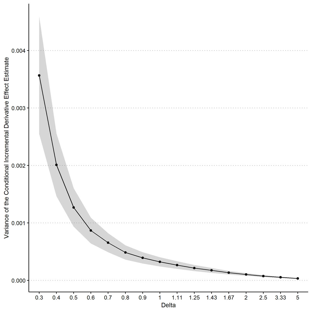
V-CIDE vs
6 Discussion
In this work, we introduced three conditional effects based on incremental propensity score interventions – the conditional incremental effect (CIE), conditional incremental contrast effect (CICE), and conditional incremental derivative effect (CIDE). We proposed two estimators, the Projection-Learner and the I-DR-Learner, which can be used to estimate any of the three conditional effects. We showed that the Projection-Learner, a projection approach, achieves parametric efficiency under weak
Finally, we illustrated our methods with a real data analysis of the effect of ICU admission on mortality conditional on a patient’s risk score. This analysis demonstrated that estimating counterfactual mean outcomes across a spectrum of incremental interventions can be more informative than just estimating the ATE. We found evidence that the ATE is positive, suggesting that sending no one to the ICU is better than sending everyone to the ICU in terms of average mortality rates. However, by examining the spectrum of incremental interventions, we estimated that average mortality changes little with mild changes in ICU admission rates. Further, we found that there is indeed statistically significant treatment effect heterogeneity across patient risk scores, but the magnitude of heterogeneity is small. An additional limitation of this analysis is that it assumed there were no unmeasured confounders, which might be implausible. The sensitivity of the results to possible unmeasured confounders could be examined in future work. To our knowledge, sensitivity analyses for incremental propensity score interventions have not yet been developed.
There are other interesting avenues for future investigation. Here we proposed CIE estimators with the simplest data generating setup – one time point and binary treatment. Several natural extensions of this work to more complex frameworks are (i) time-varying data, (ii) incremental parameters that can depend on covariate data or past data, and (iii) multi-valued or continuous treatments with different stochastic interventions. Since positivity violations are almost guaranteed with time-varying data or multi-valued or continuous treatment, it would also be important to understand how nonparametric estimators behave and how projection approaches might be utilized to approximate ATE-style effects when positivity is violated.
Acknowledgements
The authors thank the Causal Inference Reading Group at Carnegie Mellon University and several anonymous reviewers for helpful discussion and comments, and Luke Keele for guidance on the (SPOT)light study data.
-
Funding information: The authors state no funding involved.
-
Conflict of interest: The authors state no conflict of interest.
Appendix A Stability condition for Theorem 2
In this section, we state the stability condition invoked in Section 3.2 and Theorem 2. This stability condition is described in detail in Section 3 of Kennedy [3], and can be viewed as a form of stochastic equicontinuity for nonparametric regression.
Definition 1
(Stability) Suppose
wherever
Definition 1 says that the difference between the regression estimate with estimated outcomes (
where
B Estimator for the variance of the conditional incremental derivative effect (V-CIDE) when the conditioning covariate is a strict subset of all covariates
In this section, we briefly outline an estimator for the V-CIDE when the conditioning covariates
By the definition of the variance and iterated expectation,
The squared expectation term,
Lemma 3
Under Assumptions
1
and
2, the un-centered efficient influence function for
where
This result suggests the following estimator:
And, combined with the results in Sections 3.2 and 4, suggests the following estimator for the V-CIDE:
Algorithm 4
(V-CIDE Estimator when
On the training data
In the estimation sample
This estimator satisfies a similar double robustness condition to the estimator outlined in Section 4, but includes a dependence on
Theorem 4
Let
then
where
where
The theorem shows that the estimator for the V-CIDE satisfies a version of double robustness under relatively weak conditions. The result shows that our estimator attains
Like the estimator from Algorithm 3, the estimator in Algorithm 4 converges to a degenerate distribution when the V-CIDE equals zero. As discussed at the end of Section 4, we can construct a valid test for any treatment effect heterogeneity by overestimating the variance of the estimator
where
C Simulations for the Projection-Learner and I-DR-learner
In this section, we study the performance of the Projection-Learner and I-DR-Learner for estimating the conditional incremental contrast effect (CICE) with
which corresponds to the difference between the counterfactual mean outcomes when the odds of treatment are multiplied by 5 minus the counterfactual mean outcome when the odds of treatment are divided by 5. For all the analyses, we simulate 1,000 times datasets of sizes
and the CATE is defined implicitly as
which follows from the identification result in Proposition 1. Each simulated dataset
The data generating process is also illustrated in Figure A1. The covariate data

Data generating process.
We simulated estimates for the propensity scores and regression functions by adding noise, parameterized by
The
First, we compare the I-DR-Learner to the oracle estimator (“Oracle I-DR-Learner”) and a baseline learner (“Baseline CICE”) in terms of integrated mean squared error (MSE). The oracle estimator constructs the true influence function value from
This is motivated by causal identification, such as the result in Proposition 1, and does not make use of the efficient influence function for the relevant average effect. The baseline estimator for the CATE was previously examined in the literature, and has been referred to as the “T-Learner” [4].
The results of these simulations are summarized in Figure A2. Each different panel corresponds to a different convergence rate

Comparing CICE estimators.
Figure A2 illustrates the phenomenon anticipated by Theorem 2. The oracle estimator performs the best, which we would expect since it has access to the true nuisance functions. The I-DR-Learner performs the next best, and its error approaches that of the oracle estimator as
C.1 Coverage of the Projection-Learner
In this subsection, we outline results for the Projection-Learner. Specifically, we show that the projection-learner achieves approximately correct coverage for the true coefficients in the model. The true model is
and the working model is
Since the working model is well-specified, the Projection-Learner estimates the true coefficients. Figure A3 shows the coverage of 95% confidence intervals constructed for each coefficient using the sandwich variance as in Corollary 2. When the nuisance function estimators have large error, such that

Coverage of Projection-Learner confidence intervals for coefficient estimates.
D Proofs for results in Section 2
Proposition 2
Let
where
Proof
We have
where the first line follows by definition, the second by Assumptions 1 and 2, and the third and final line by exchanging expectation and derivative, taking the derivative with respect to
E Proofs for results in Section 3
Lemma 1
Under Assumptions
1
and
2, the un-centered efficient influence function for the average incremental derivative effect,
where
Proof
We prove the result by showing that
Let
where
where
By iterated expectations and rearranging,
where
It can be shown that
We show this in the postscript to this proof. Here we provide some intuition. It is clear that the first line of (43) is already a second order. The second line of (43) is second order because
Now, we relate
for
with
since
which shows that
Since the model is nonparametric, the tangent space is the entire Hilbert space of mean-zero finite-variance functions, and so there is only one influence function satisfying (44) and it is the efficient one [32]. Therefore,
Below, we show the algebra for why
Therefore, letting
For the second line in (43), we have
Finally, revisiting the first line of (43),
E.1 Efficient influence functions for the average incremental effect and the average incremental contrast effect
By Corollary 2 in the study by Kennedy [11], the efficient influence function for the average incremental effect is
and the efficient influence function for the average incremental contrast effect is
Corollary 1
Let
where
Proof
Let
where
Following essentially the same logic as in Lemma 1, by iterated expectations and rearranging,
This second order term can be expressed as a product of errors, as is shown in post script to the proof for Lemma 1. Therefore, since our model is nonparametric,
Theorem 1
Let
The function class
The estimators are consistent in the sense that
The map
where
Proof
This proof follows closely both Lemma 3 from the study by Kennedy et al. [45] and Theorem 5.31 of the study by van der Vaart [34]. Since
By adding and subtracting on the right hand side of the equation above, omitting
The first term appears directly in the statement in the theorem, so we will not manipulate it. It is a sample average of a fixed function, and so by the central limit theorem it will be asymptotically Gaussian. The second and third terms are empirical process terms. The fourth term can be linearized in
First, we will tackle the second and third terms. Under the Donsker and consistency conditions in Assumptions (c) and (d), the second term is
The fourth term, by the differentiability of the map
where the first line is a first-order Taylor expansion about
Bringing everything together,
Re-arranging, we have that
We can re-arrange and by the non-singularity of the derivative matrix
To address the
so that
and therefore
and
Finally, plugging these results back into equation (48), we have
And, adding back in all arguments, we can conclude
which provides the first statement of the theorem.
For the second statement, recall that
The final result follows by Cauchy–Schwartz and a boundedness condition, which depends on the target estimand. If the estimand is a projection of the CIDE, then the result follows by equivalent logic to the proof of Lemma 1 and the first part of Assumption (a), which says that the estimated CATE is bounded. If, instead, the estimand is a projection of the CIE or the CICE, the result follows by equivalent logic to the proofs of Lemmas 5 and 6 in the appendix of the study by Kennedy [11] and the second part of Assumption (a), which says that the true CATE is bounded.□
Theorem 2
Let
for
and
Proof
This follows from Proposition 1 of the study by Kennedy [3], the definition of
The bounded functions in
where
When
where
F Proofs for results in Section 4
Lemma 2
Under Assumptions
1
and
2, the un-centered efficient influence function for
where
Proof
As in Lemma 1, we prove this result by showing that the estimand admits a von Mises expansion where the second-order term is a product of errors.
Omitting arguments, let
where
and
Theorem 3
Let
then
where
Proof
First, note that, by construction
where the second line follows by defining
Similarly, by construction,
Therefore, if we define
Then, by adding and subtracting terms, we have the usual expansion
where the first term on the right hand side of the final equation will follow a central limit theorem, the second term is an empirical process term, and the third term is a bias term.
Starting with the third term, we see
where the second line follows by the proof of Lemma 2. For the second term on the final line above, we see that
where the fourth line follows by Assumption (a), the fifth line because
The second term from equation (49), the empirical process term, is simpler to bound. By Lemma 2 of the study by Kennedy et al. [79] and by sample splitting, we have
By the triangle inequality
where the last line follows by Assumption (a), which says that
Therefore, by the central limit theorem,
with
Proposition 4
Let
Under Assumptions 1 and 2, Assumption (a) from Theorem 1, and Assumption (a) from Theorem 3. If
then
where
Proof
This result follows by Lemmas 1 and 2, the conditions of the Proposition, and the Delta method (for the second convergence result).□
Proposition 5
Let
so that
Proof
By the assumption that
Therefore, when
And so,
which implies the result.□
Proposition 3
Under Assumptions 1 and 2, Assumption (a) from Theorem 1, and Assumption (a) from Theorem 3, if
then the asymptotic Type I error rate of the test in (28) is less than or equal to
Proof
By definition,
where
where
By Proposition 5, when
Therefore, since
which implies that the asymptotic Type I error of the test in (28) is less than or equal to
References
[1] Athey S, Imbens G. Recursive partitioning for heterogeneous causal effects. Proc National Acad Sci. 2016;113(27):7353–60. 10.1073/pnas.1510489113Search in Google Scholar PubMed PubMed Central
[2] Foster DJ, Syrgkanis V. Orthogonal statistical learning. Ann Stat. 2023;51(3):879–908. 10.1214/23-AOS2258Search in Google Scholar
[3] Kennedy EH. Towards optimal doubly robust estimation of heterogeneous causal effects. 2020. arXiv: http://arXiv.org/abs/arXiv:2004.14497. Search in Google Scholar
[4] Künzel SR, Sekhon JS, Bickel PJ, Yu B. Metalearners for estimating heterogeneous treatment effects using machine learning. Proc Nat Acad Sci. 2019;116(10):4156–65. 10.1073/pnas.1804597116Search in Google Scholar PubMed PubMed Central
[5] Nie X, Wager S. Quasi-oracle estimation of heterogeneous treatment effects. Biometrika. 2021;108(2):299–319. 10.1093/biomet/asaa076Search in Google Scholar
[6] Semenova V, Chernozhukov V. Debiased machine learning of conditional average treatment effects and other causal functions. Econom J. 2021;24(2):264–89. 10.1093/ectj/utaa027Search in Google Scholar
[7] Shalit U, Johansson FD, Sontag D. Estimating individual treatment effect: generalization bounds and algorithms. In: International Conference on Machine Learning. PMLR; 2017. p. 3076–85. Search in Google Scholar
[8] Keele L, Harris S, Grieve R. Does transfer to intensive care units reduce mortality? A comparison of an instrumental variables design to risk adjustment. Medical Care. 2019;57(11):e73–9. 10.1097/MLR.0000000000001093Search in Google Scholar PubMed
[9] Díaz I, Hejazi NS. Causal mediation analysis for stochastic interventions. J R Stat Soc Ser B Stat Methodol. 2020;82(3):661–83. 10.1111/rssb.12362Search in Google Scholar
[10] Haneuse S, Rotnitzky A. Estimation of the effect of interventions that modify the received treatment. Stat Med. 2013;32(30):5260–77. 10.1002/sim.5907Search in Google Scholar PubMed
[11] Kennedy EH. Nonparametric causal effects based on incremental propensity score interventions. J Amer Stat Assoc. 2019;114(526):645–56. 10.1080/01621459.2017.1422737Search in Google Scholar
[12] Moore KL, Neugebauer R, van der Laan MJ, Tager IB. Causal inference in epidemiological studies with strong confounding. Stat Med. 2012;31(13):1380–404. 10.1002/sim.4469Search in Google Scholar PubMed PubMed Central
[13] Muñoz ID, van der Laan M. Population intervention causal effects based on stochastic interventions. Biometrics. 2012;68(2):541–9. 10.1111/j.1541-0420.2011.01685.xSearch in Google Scholar PubMed PubMed Central
[14] Young JG, Hernán MA, Robins JM. Identification, estimation and approximation of risk under interventions that depend on the natural value of treatment using observational data. Epidemiol Methods. 2014;3(1):1–9. 10.1515/em-2012-0001Search in Google Scholar PubMed PubMed Central
[15] Zhou X, Opacic A. Marginal interventional effects. 2022. arXiv: http://arXiv.org/abs/arXiv:2206.10717. Search in Google Scholar
[16] Bonvini M, McClean A, Branson Z, Kennedy EH. Incremental causal effects: an introduction and review. In: Handbook of Matching and Weighting Adjustments for Causal Inference. New York, USA: Chapman and Hall/CRC; 2023. p. 349–72. 10.1201/9781003102670-18Search in Google Scholar
[17] Wen L, Marcus JL, Young JG. Intervention treatment distributions that depend on the observed treatment process and model double robustness in causal survival analysis. Stat Methods Med Res. 2023;32(3):509–23. 10.1177/09622802221146311Search in Google Scholar PubMed PubMed Central
[18] Westreich D, Cole SR. Invited commentary: positivity in practice. Amer J Epidemiol. 2010;171(6):674–7. 10.1093/aje/kwp436Search in Google Scholar PubMed PubMed Central
[19] Stensrud MJ, Laurendeau J, Sarvet AL. Optimal regimes for algorithm-assisted human decision-making. 2022. arXiv: http://arXiv.org/abs/arXiv:2203.03020. Search in Google Scholar
[20] R Core Team. A Language and Environment for Statistical Computing. 2023. R Foundation for Statistical Computing. Search in Google Scholar
[21] Kennedy EH. npcausal: Nonparametric Causal Inference Methods [Internet]. 2021. [cited 2023 Sept 20]. https://github.com/ehkennedy/npcausal/. Search in Google Scholar
[22] Kim K, Kennedy EH, Naimi AI. Incremental intervention effects in studies with dropout and many timepoints. J Causal Infer. 2021;9(1):302–44. 10.1515/jci-2020-0031Search in Google Scholar
[23] Sarvet AL, Wanis KN, Young JG, Hernandez-Alejandro R, Stensrud MJ. Longitudinal incremental propensity score interventions for limited resource settings. Wiley Online Library; 2023. 10.1111/biom.13859Search in Google Scholar PubMed
[24] Rudolph JE, Kim K, Kennedy EH, Naimi AI. Estimation of the time-varying incremental effect of low-dose aspirin on incidence of pregnancy. Epidemiology. 2022;34(1):38–44. 10.1097/EDE.0000000000001545Search in Google Scholar PubMed PubMed Central
[25] Chakraborty B, Murphy SA. Dynamic treatment regimes. Ann Rev Stat Appl. 2014;1:447–64. 10.1146/annurev-statistics-022513-115553Search in Google Scholar PubMed PubMed Central
[26] Murphy SA. Optimal dynamic treatment regimes. J R Stat Soc Ser B Stat Methodol. 2003;65(2):331–55. 10.1111/1467-9868.00389Search in Google Scholar
[27] Díaz I, Williams N, Hoffman KL, Schenck EJ. Nonparametric causal effects based on longitudinal modified treatment policies. J Amer Stat Assoc. 2023;118(542):846–57. 10.1080/01621459.2021.1955691Search in Google Scholar
[28] Taubman SL, Robins JM, Mittleman MA, Hernán MA. Intervening on risk factors for coronary heart disease: an application of the parametric g-formula. Int J Epidemiol. 2009;38(6):1599–611. 10.1093/ije/dyp192Search in Google Scholar PubMed PubMed Central
[29] Robins JM, Hernán MA, Siebert U. Effects of multiple interventions. In: Ezzati M, Lopez AD, Rodgers AA, Murray CJ. Comparative Quantification of Health Risks: Global and Regional Burden of Disease Attributable to Selected Major Risk Factors. Geneva, Switzerland: World Health Organization; 2004. p. 2191–230. Search in Google Scholar
[30] Vansteelandt S, Bekaert M, Claeskens G. On model selection and model misspecification in causal inference. Stat Meth Med Res. 2012;21(1):7–30. 10.1177/0962280210387717Search in Google Scholar PubMed
[31] Bickel PJ, Klaassen CA, Ritov YA, Wellner JA. Efficient and adaptive estimation for semiparametric models. Baltimore: Johns Hopkins University Press; 1993. Search in Google Scholar
[32] Tsiatis AA. Semiparametric theory and missing data. New York: Springer; 2006. Search in Google Scholar
[33] van der Laan MJ, Robins JM. Unified methods for censored longitudinal data and causality. New York: Springer; 2003. 10.1007/978-0-387-21700-0Search in Google Scholar
[34] van der Vaart AW Asymptotic statistics. Cambridge: Cambridge University Press; 2000. Search in Google Scholar
[35] van der Vaart AW. Semiparametric statistics. In: Lectures on Probability Theory and Statistics. Berlin: Springer; 2002. p. 331–457. Search in Google Scholar
[36] Mises RV. On the asymptotic distribution of differentiable statistical functions. Ann Math Stat. 1947;18(3):309–48. 10.1214/aoms/1177730385Search in Google Scholar
[37] Chernozhukov V, Chetverikov D, Demirer M, Duflo E, Hansen C, Newey W, et al. Double/debiased machine learning for treatment and structural parameters. Econom J. 2018;21(1):C1–C68. 10.1111/ectj.12097Search in Google Scholar
[38] Kennedy EH. Semiparametric doubly robust targeted double machine learning: a review. 2022. arXiv: http://arXiv.org/abs/arXiv:2203.06469. Search in Google Scholar
[39] Beran R. Minimum Hellinger distance estimates for parametric models. Ann Stat. 1977;5:445–63. 10.1214/aos/1176343842Search in Google Scholar
[40] Berk R, Buja A, Brown L, George E, Kuchibhotla AK, Su W, et al. Assumption lean regression. Amer Stat. 2019;75(1):76–84. 10.1080/00031305.2019.1592781Search in Google Scholar
[41] Buja A, Brown L, Kuchibhotla AK, Berk R, George E, Zhao L. Models as approximations II. Stat Sci. 2019;34(4):545–65. 10.1214/18-STS694Search in Google Scholar
[42] Huber PJ. The behavior of maximum likelihood estimates under nonstandard conditions. In: Proceedings of the Fifth Berkeley Symposium on Mathematical Statistics and Probability. 1967; (Vol. 1. Issue No. 1) pp. 221–33. Search in Google Scholar
[43] White H. Using least squares to approximate unknown regression functions. Int Econom Rev. 1980;21(1):149–70. 10.2307/2526245Search in Google Scholar
[44] Cuellar M, Kennedy EH. A non-parametric projection-based estimator for the probability of causation, with application to water sanitation in Kenya. J R Stat Soc Ser A Stat Soc. 2020;183(4):1793–818. 10.1111/rssa.12548Search in Google Scholar
[45] Kennedy EH, Balakrishnan S, Wasserman LA. Semiparametric counterfactual density estimation. Biometrika. 2023;110:asad017. 10.1093/biomet/asad017Search in Google Scholar
[46] Petersen M, Schwab J, Gruber S, Blaser N, Schomaker M, van der Laan MJ. Targeted maximum likelihood estimation for dynamic and static longitudinal marginal structural working models. J Causal Infer. 2014;2(2):147–85. 10.1515/jci-2013-0007Search in Google Scholar PubMed PubMed Central
[47] Neugebauer R, van der Laan M. Nonparametric causal effects based on marginal structural models. J Stat Plan Inference. 2007;137(2):419–34. 10.1016/j.jspi.2005.12.008Search in Google Scholar
[48] Vansteelandt S, Dukes O. Assumption-lean inference for generalised linear model parameters. J R Stat Soc Ser B Stat Methodol. 2022;84(3):657–85. 10.1111/rssb.12504Search in Google Scholar
[49] Hahn PR, Murray JS, Carvalho CM. Bayesian regression tree models for causal inference: Regularization, confounding, and heterogeneous effects (with discussion). Bayesian Anal. 2020;15(3):965–1056. 10.1214/19-BA1195Search in Google Scholar
[50] Zimmert M, Lechner M. Nonparametric estimation of causal heterogeneity under high-dimensional confounding. 2019. arXiv: http://arXiv.org/abs/arXiv:1908.08779. Search in Google Scholar
[51] Hines O, Dukes O, Diaz-Ordaz K, Vansteelandt S. Demystifying statistical learning based on efficient influence functions. Amer Stat. 2022;76(3):292–304. 10.1080/00031305.2021.2021984Search in Google Scholar
[52] Robins JM. Correcting for non-compliance in randomized trials using structural nested mean models. Commun Stat-Theory Methods. 1994;23(8):2379–412. 10.1080/03610929408831393Search in Google Scholar
[53] Robins JM, Mark SD, Newey WK. Estimating exposure effects by modelling the expectation of exposure conditional on confounders. Biometrics. 1992;48:479–95. 10.2307/2532304Search in Google Scholar
[54] Robinson PM. Root-N-consistent semiparametric regression. Econometrica: J Econometric Soc. 1988;56:931–54. 10.2307/1912705Search in Google Scholar
[55] Vansteelandt S, Joffe M. Structural nested models and g-estimation: the partially realized promise. Stat Sci. 2014;29(4):707–31. 10.1214/14-STS493Search in Google Scholar
[56] Chen Q, Syrgkanis V, Austern M. Debiased machine learning without sample-splitting for stable estimators. Adv Neural Inform Process Syst. 2022;35:3096–109. Search in Google Scholar
[57] van der Vaart AW, Wellner JA. Weak convergence and empirical processes. New York, USA: Springer; 1996. 10.1007/978-1-4757-2545-2Search in Google Scholar
[58] Robins J, Li L, Tchetgen Tchetgen E, van der Vaart A. Higher order influence functions and minimax estimation of nonlinear functionals. In: Probability and statistics: essays in honor of David A. Freedman. Beechwood, Ohio, USA: Institute of Mathematical Statistics. 2008. Vol. 2. p. 335–422. 10.1214/193940307000000527Search in Google Scholar
[59] Zheng W, van der Laan MJ. Asymptotic theory for cross-validated targeted maximum likelihood estimation. U.C. Berkeley Division of Biostatistics Working Paper Series. 2010. Paper 273. 10.2202/1557-4679.1181Search in Google Scholar PubMed PubMed Central
[60] Birgé L, Massart P. Estimation of integral functionals of a density. Ann Stat. 1995;23(1):11–29. 10.1214/aos/1176324452Search in Google Scholar
[61] Farrell MH. Robust inference on average treatment effects with possibly more covariates than observations. J Econometrics. 2015;189(1):1–23. 10.1016/j.jeconom.2015.06.017Search in Google Scholar
[62] Tibshirani R. Regression shrinkage and selection via the lasso. J R Stat Soc Ser B Stat Methodol. 1996;58(1):267–88. 10.1111/j.2517-6161.1996.tb02080.xSearch in Google Scholar
[63] Tsybakov AB. Introduction to nonparametric estimation. New York: Springer; 2009. 10.1007/b13794Search in Google Scholar
[64] Wasserman L. All of nonparametric statistics. New York, USA: Springer Science & Business Media; 2006. Search in Google Scholar
[65] Crump RK, Hotz VJ, Imbens GW, Mitnik OA. Nonparametric tests for treatment effect heterogeneity. Rev Econom Stat. 2008;90(3):389–405. 10.1162/rest.90.3.389Search in Google Scholar
[66] Ding P, Feller A, Miratrix L. Randomization inference for treatment effect variation. J R Stat Soc Ser B Stat Methodol. 2016;78(3):655–71. 10.1111/rssb.12124Search in Google Scholar
[67] Ding P, Feller A, Miratrix L. Decomposing treatment effect variation. J Amer Stat Assoc. 2019;114(525):304–17. 10.1080/01621459.2017.1407322Search in Google Scholar
[68] Luedtke A, Carone M, van der Laan MJ. An omnibus non-parametric test of equality in distribution for unknown functions. J R Stat Soc Ser B Stat Methodol. 2019;81(1):75–99. 10.1111/rssb.12299Search in Google Scholar PubMed PubMed Central
[69] Williamson BD, Gilbert PB, Simon NR, Carone M. A general framework for inference on algorithm-agnostic variable importance. J Amer Stat Assoc. 2023;118(543):1645–58. 10.1080/01621459.2021.2003200Search in Google Scholar PubMed PubMed Central
[70] Harris S, Singer M, Sanderson C, Grieve R, Harrison D, Rowan K. Impact on mortality of prompt admission to critical care for deteriorating ward patients: an instrumental variable analysis using critical care bed strain. Intensive Care Med. 2018;44:606–15. 10.1007/s00134-018-5148-2Search in Google Scholar PubMed PubMed Central
[71] Gabler NB, Ratcliffe SJ, Wagner J, Asch DA, Rubenfeld GD, Angus DC, et al. Mortality among patients admitted to strained intensive care units. Am J Respiratory Critical Care Med. 2013;188(7):800–6. 10.1164/rccm.201304-0622OCSearch in Google Scholar PubMed PubMed Central
[72] Renaud B, Santin A, Coma E, Camus N, Van Pelt D, Hayon J, et al. Association between timing of intensive care unit admission and outcomes for emergency department patients with community-acquired pneumonia. Critical Care Medicine. 2009;37(11):2867–74. 10.1097/CCM.0b013e3181b02dbbSearch in Google Scholar PubMed
[73] Harrison DA, Parry GJ, Carpenter JR, Short A, Rowan K. A new risk prediction model for critical care: the Intensive Care National Audit & Research Centre (ICNARC) model. Crit Care Med. 2007;35(4):1091–8. 10.1097/01.CCM.0000259468.24532.44Search in Google Scholar PubMed
[74] Williams B, Alberti G, Ball C, Ball D, Binks R, Durham L. National Early Warning Score (NEWS). Standardising the assessment of acute-illness severity in the NHS. London, UK: Royal College of Physicians; 2012. Search in Google Scholar
[75] Vincent JL, Moreno R, Takala J, Willatts S, De Mendonça A, Bruining H, et al. The SOFA (Sepsis-related Organ Failure Assessment) score to describe organ dysfunction/failure: On behalf of the Working Group on Sepsis-Related Problems of the European Society of Intensive Care Medicine. 1996. 10.1007/BF01709751Search in Google Scholar PubMed
[76] Kang H, Jiang Y, Zhao Q, Small D. ivmodel: Statistical Inference and Sensitivity Analysis for Instrumental Variables Model [Internet]. 2023 [cited 2023 Oct 25]. https://cran.r-project.org/web/packages/ivmodel/. Search in Google Scholar
[77] Wright MN, Ziegler A. Ranger: a fast implementation of random forests for high dimensional data in C++ and R. J Stat Software. 2017;77(1):1–17. 10.18637/jss.v077.i01Search in Google Scholar
[78] Wood S. mgcv: Mixed GAM computation vehicle with GCV/AIC/REML smoothness estimation. 2012. Search in Google Scholar
[79] Kennedy EH, Balakrishnan S, G’Sell M. Sharp instruments for classifying compliers and generalizing causal effects. Ann Stat. 2020;48(4):2008–30. 10.1214/19-AOS1874Search in Google Scholar
© 2024 the author(s), published by De Gruyter
This work is licensed under the Creative Commons Attribution 4.0 International License.
Articles in the same Issue
- Research Articles
- Evaluating Boolean relationships in Configurational Comparative Methods
- Doubly weighted M-estimation for nonrandom assignment and missing outcomes
- Regression(s) discontinuity: Using bootstrap aggregation to yield estimates of RD treatment effects
- Energy balancing of covariate distributions
- A phenomenological account for causality in terms of elementary actions
- Nonparametric estimation of conditional incremental effects
- Conditional generative adversarial networks for individualized causal mediation analysis
- Mediation analyses for the effect of antibodies in vaccination
- Sharp bounds for causal effects based on Ding and VanderWeele's sensitivity parameters
- Detecting treatment interference under K-nearest-neighbors interference
- Bias formulas for violations of proximal identification assumptions in a linear structural equation model
- Current philosophical perspectives on drug approval in the real world
- Foundations of causal discovery on groups of variables
- Improved sensitivity bounds for mediation under unmeasured mediator–outcome confounding
- Potential outcomes and decision-theoretic foundations for statistical causality: Response to Richardson and Robins
- Quantifying the quality of configurational causal models
- Design-based RCT estimators and central limit theorems for baseline subgroup and related analyses
- An optimal transport approach to estimating causal effects via nonlinear difference-in-differences
- Estimation of network treatment effects with non-ignorable missing confounders
- Double machine learning and design in batch adaptive experiments
- The functional average treatment effect
- An approach to nonparametric inference on the causal dose–response function
- Review Article
- Comparison of open-source software for producing directed acyclic graphs
- Special Issue on Neyman (1923) and its influences on causal inference
- Optimal allocation of sample size for randomization-based inference from 2K factorial designs
- Direct, indirect, and interaction effects based on principal stratification with a binary mediator
- Interactive identification of individuals with positive treatment effect while controlling false discoveries
- Neyman meets causal machine learning: Experimental evaluation of individualized treatment rules
- From urn models to box models: Making Neyman's (1923) insights accessible
- Prospective and retrospective causal inferences based on the potential outcome framework
- Causal inference with textual data: A quasi-experimental design assessing the association between author metadata and acceptance among ICLR submissions from 2017 to 2022
- Some theoretical foundations for the design and analysis of randomized experiments