Conditional generative adversarial networks for individualized causal mediation analysis
-
Cheng Huan


Abstract
Most classical methods popularly used in causal mediation analysis can only estimate the average causal effects and are difficult to apply to precision medicine. Although identifying heterogeneous causal effects has received some attention, the causal effects are explored using the assumptive parametric models with limited model flexibility and analytic power. Recently, machine learning is becoming a major tool for accurately estimating individualized causal effects, thanks to its flexibility in model forms and efficiency in capturing complex nonlinear relationships. In this article, we propose a novel method, conditional generative adversarial network (CGAN) for individualized causal mediation analysis (CGAN-ICMA), to infer individualized causal effects based on the CGAN framework. Simulation studies show that CGAN-ICMA outperforms five other state-of-the-art methods, including linear regression, k-nearest neighbor, support vector machine regression, decision tree, and random forest regression. The proposed model is then applied to a study on the Alzheimer’s disease neuroimaging initiative dataset. The application further demonstrates the utility of the proposed method in estimating the individualized causal effects of the apolipoprotein E-ε4 allele on cognitive impairment directly or through mediators.
1 Introduction
Mediation analysis has been widely applied in biomedical [1–4], epidemiology [5,6], and social-psychological studies [7–9]. Its initial idea can be at least dated back to Woodworth’s stimulus-response model in dynamic psychology in 1929 [10] and Wright’s path analysis in statistics in 1934 [11]. Conceptually, mediation analysis is an effective statistical tool that investigates the underlying mechanism of how an exposure exerts its effects on the outcome of interest [12,13]. Specifically, an exposure may affect the outcome of interest directly or indirectly through some intermediate variables, commonly referred to as mediators. The exposure’s total effect (TE) on the outcome of interest can be decomposed into direct and indirect effects. Then, the counterfactual framework, also known as the potential outcome framework or Rubin’s model [14–17], for mediation analysis is proposed to identify the direct and indirect effects. Such mediation analysis is called the causal mediation analysis and is under study in this article. Causal mediation analysis allows researchers to build various methods to accommodate different outcome types, such as discrete, continuous, and time-to-event outcomes.
In recent years, there have been a growing number of studies in causal mediation analysis that focus on the average causal effects. Various methods have been developed, including parametric [3,4,18–20], semiparametric [1,21,22], and nonparametric models [23]. However, given the prevalence of personalized medicine, it is also interesting to look beyond the average causal effects to estimate the conditional average causal effects or individualized causal effects (ICEs) and further understand how the causal effects vary with observable characteristics. Typical examples include accommodation of exposure–mediator interaction into the outcome regression model [16,24] and conditional direct/indirect effects given the covariates level [25,26]. Estimating ICEs can be particularly challenging for two main reasons. First, a common framework for causal mediation analysis is the counterfactual framework [14–16], where potential mediators contain both factual and counterfactual mediators, and potential outcomes contain both factual and counterfactual outcomes. However, we can only observe the factual mediators and outcomes but never counterfactual mediators and outcomes. Second, the functional forms of causal effects are often nonlinear and unknown, but statistical methods for causal mediation analysis to deal with unknown nonlinear functions are still lacking. Park and Kaplan [27] combined Bayesian inferential methods with G-computation to conduct Bayesian causal mediation analysis for group randomized designs with homogeneous and heterogeneous effects. Qin and Hong [28] developed a weighting method to identify and estimate site-specific mediation effects using inverse-probability-of-treatment weight [29] and ratio-of-mediator-probability weighting [30]. Later on, Dyachenko and Allenby [31] proposed a Bayesian mixture model combining likelihood functions based on two different outcome models. Xue et al. [32] suggested a novel mediation penalty to jointly incorporate effects in mediator and outcome models for high-dimensional data. Qin and Wang [33] proposed general definitions of causal conditional effects with moderated mediation effects and conducted estimations of the indirect and direct effects across subgroups. Although these methods for estimating heterogeneous causal effects have been proven helpful in many situations, they also have limitations. For example, some of these methods [27,32] rely heavily on the structure of linear structural equation modeling (LSEM), which may not accurately capture the complexity of real-world systems. Qin and Hong [28] focused on estimating the population average and between-site variance of indirect and direct effects. However, their analysis did not extend to estimating these effects for different subpopulations. Qin and Wang [33] rely on correct specifications of the parametric mediator and outcome models for estimating and inferring causal effects. Other methods, such as the one proposed by Dyachenko and Allenby [31], require a prespecified number of subgroups and only consider a single mediator variable. To address these limitations, we explore alternative modeling frameworks that can better capture the complexity of real-world systems in terms of relaxing the linear assumption, allowing more general forms of heterogeneity, and accommodating multiple mediators. These improvements can enhance the flexibility and generalizability of causal mediation analysis and allow for more accurate estimation of heterogeneous causal effects.
Recently, machine learning has triggered our interest, which does not presuppose the model forms and can effectively capture complex nonlinear relationships. It has achieved widespread success in many fields, such as computer vision [34] and natural language processing [35]. Integrating machine learning and statistical methods has also received much attention. In causal inference, for example, Chen and Liu [36] proposed a specific network to evaluate the heterogeneous treatment effect. Chen et al. [37] further used deep representation learning to estimate the individualized treatment effect (ITE). In addition, Chu et al. [38] developed an adversarial deep treatment effect prediction model, and Ge et al. [39] modified the conditional generative adversarial networks (CGANs) to estimate ITE. In particular, Yoon et al. [40] proposed a CGAN-based deep learning approach called conditional generative adversarial nets for inference of individualized treatment effects (GANITE). This approach consists of two blocks: a counterfactual imputation block and an ITE block, each of which consists of a generator and a discriminator. Despite its superior utility in identifying ITEs, this method did not consider mediators and is thus inapplicable to the mediation analysis in this study.
We propose a novel approach, CGAN for individualized causal mediation analysis (CGAN-ICMA), to estimate ICEs and explore the individualized causal mechanism. The proposed method consists of two main components: a mediator block and an outcome block, where the framework within each component is similar to GANITE. The mediator block consists of two subblocks: a counterfactual mediator block, including a counterfactual mediator generator
This study is motivated by the Alzheimer’s disease (AD) neuroimaging initiative (ADNI) dataset, which recruited approximately 800 subjects between 55 and 80 years old initially and collected imaging, genetic biomarkers, and cognitive data from subjects. Among the biological variables, the apolipoprotein E-
The work is structured as follows. Section 2 briefly reviews ICEs and several assumptions in the mediation analysis and the problem formulation. Section 3 elucidates the proposed CGAN-ICMA method. In Section 4, we evaluate the empirical performance of the proposed method by comparing it with various state-of-the-art approaches, including linear regression (LR), k-nearest neighbor (KNN), support vector machine regression (SVM), decision tree (DT), and random forest regression (RF), through simulation studies. To further evaluate the performance, we apply the proposed method to the ADNI dataset to investigate the ICEs of carrying the APOE-
2 Individualized causal effects
In Section 2.1, we begin by briefly reviewing the standard causal mediation analysis with multiple mediators and defining the individualized direct, indirect, and TE [15,16,48] of interest under the potential outcomes framework. Then, in Section 2.2, we introduce a set of assumptions [16,48,49] in the mediation analysis and the problem formulation.
2.1 Definitions
Let
where
Next, we define the individualized natural direct effect (NDE) for the
and the individualized TE for the
Again, in the real data analysis of this article,
Therefore, the NIE under one treatment state and the NDE under the other treatment state add up to the TE. In this article, we consider the decomposition with
The NIE defined earlier can be further broken into
Similar to the decomposition proposed by Wang et al. [48], there are
2.2 Assumptions and problem formulation
We now introduce several assumptions [16,48,49] in the mediation analysis to identify the direct and indirect effects. The first assumption stated in the following is called the stable unit treatment value assumption (SUTVA).
Assumption 1
(SUTVA)
The potential outcomes for any unit do not vary with the treatments assigned to other units;
For each unit, there are no different forms or versions of each treatment level, which lead to different potential outcomes.
These two elements of SUTVA enable us to exploit the presence of multiple units for estimating causal effects. The second assumption is to guarantee that the probability of being assigned to each treatment arm is positive for every subject.
Assumption 2
(Overlap). For all
Denote the potential mediators by
Assumption 3
(Unconfoundedness)
for each
It follows from the aforementioned assumptions that
such that the ICEs can be identified through the expected potential outcomes as long as the joint distribution of the potential mediators,
In general case with multiple mediators (
Then, we look at the integral in equation (6). Assuming the mediator–outcome relationship is linear, we can move the expectation in equation (6) outside the integral sign. This allows us to obtain the expected potential outcomes by estimating the conditional expectation of
We clarify that the linear assumption on the mediator–outcome relationship aims at resolving the challenge of computing the integral in equation (6) through the joint distribution, especially in the case where there are multiple mediators (
Notably, only potential mediators and potential outcomes corresponding to the assigned treatment can be observed. We call these potential mediators and potential outcomes factual mediators and factual outcomes, respectively, and call the unobservable potential mediators and potential outcomes counterfactual mediators and counterfactual outcomes, respectively. Denote the observed individualized sample as
3 CGAN-ICMA
We propose CGAN-ICMA to predict the potential outcomes given the covariates and further estimate the ICEs of interest. First, given covariates
3.1 Mediator block
We emphasize that only the potential mediators corresponding to the assigned treatment can be observed, and the counterfactual mediators are missing. So we adapt the structure of the model introduced by Yoon et al. [40] to predict the complete mediators given the covariates and further obtain the potential mediators.
First, we set up a counterfactual mediator block, including a generator and a discriminator, to generate the complete mediator vector. Next, we transfer this complete mediator vector with given covariates
3.1.1 Counterfactual mediator generator (
G
M
)
We denote by
3.1.2 Counterfactual mediator discriminator (
D
M
)
Noticing that the first component of a sample from
Now, for the observed samples, we denote the generated complete mediator vector as
where
In addition, since the generated factual mediators should be close to the observed factual mediators, an additional “supervised” loss is considered as follows:
where
where
3.1.3 Inferential mediator block (
I
M
)
After training the aforementioned counterfactual mediator block, we can obtain the complete mediator vector
In this block, the given covariates
For the observed samples, denote the corresponding mediator samples obtained by this block as
Then, the inferential mediator block is optimized as follows:
where
After introducing the first component to predict the complete mediators for the given covariates, we describe the second component, the outcome block, to predict the potential outcomes.
3.2 Outcome block
Like the mediator block, the outcome block comprises two subblocks: a counterfactual outcome block and an inferential outcome block. We briefly describe these two subblocks as follows.
3.2.1 Counterfactual outcome generator (
G
Y
)
Denote
3.2.2 Counterfactual outcome discriminator (
D
Y
)
Denote
For the observed samples, denote the generated vector of
and the “supervised” loss as follows:
Then, we iteratively optimize
where
3.2.3 Inferential outcome block (
I
Y
)
After training the aforementioned counterfactual outcome block, we can obtain the vector
In this block, we combine the given covariates
For the observed samples, denote the generated vector of this block as
and the inferential outcome block is optimized as follows:
where
Kingma and Adam [52] is chosen as the optimizer for training the aforementioned network to obtain the best performance. Once the trained model is obtained, we can predict the individualized potential outcomes given the covariates
The predicted potential mediator vector is then presented as
for the corresponding combination of

Architecture of CGAN-ICMA (
4 Simulation study
This section evaluates the empirical performance of CGAN-ICMA through simulation studies. We estimate ICEs and compare CGAN-ICMA with LR [53], KNN [54], SVM [55], DT [56], and RF [57], which are introduced in Section 4.2 based on metrics defined in Section 4.1.
4.1 Performance metrics
Yoon et al. [40] introduced an empirical precision in estimation of heterogeneous effect (PEHE) without mediators as follows:
where
Denote the observed training dataset as
and the predicted potential outcomes as follows:
for each specific choice of
A small value of
4.2 Competing methods
In this section, we provide additional information on how we implemented five competing methods, LR, KNN, SVM, DT, and RF. As our proposed method consists of a mediator block and an outcome block, it is necessary that the competing methods also include two corresponding components. First, the LR method is applied in both the mediator and outcome blocks to model the relationships between the covariates, treatment, mediator, and outcome. Specifically, the LR model in the mediator block captures the linear relationship between the mediator and the covariates and treatment, while the LR model in the outcome block captures the linear relationship between the outcome and the covariates, mediator, and treatment. We implement LR using the LinearRegression function available in the sklearn.linear_model module of Python. Similarly, the KNN method is utilized in both the mediator and outcome blocks. To implement KNN, we use the KNeighborsRegressor function provided by the sklearn.neighbors module in Python. The SVM method is applied in both the mediator and outcome blocks, and we implement SVM using the SVR function available in the sklearn.svm module of Python. Furthermore, to execute DT in both blocks, we use the DecisionTreeRegressor function provided by the the sklearn.tree module in Python. Finally, we use the RandomForestRegressor function provided by the sklearn.ensemble module in Python to implement the RT method in both blocks.
4.3 Simulation 1 (one-mediator case)
We consider two settings: one is heterogeneous, and another is homogeneous. Table S1 of the Supplementary Material summarizes the hyperparameters in the network for this simulation.
4.3.1 Setting 1 (heterogeneous setting)
where
We generate 1,000 samples from the above setting and use 900 instances for training and 100 instances for testing (i.e., n = 1,000,
Performance of six methods for estimating ICE in Simulation 1 (heterogeneous setting)
| Methods | Mean (std) based on 1,000 replications | ||
|---|---|---|---|
|
|
|
|
|
| CGAN-ICMA | 7.705 (4.771) | 2.682 (0.862) | 7.183 (4.895) |
| LR | 10.389 (5.010) | 3.812 (0.751) | 9.692 (5.155) |
| KNN(3) | 10.523 (4.226) | 5.569 (0.723) | 8.937 (4.480) |
| KNN(5) | 9.500 (4.450) | 4.659 (0.637) | 8.105 (4.679) |
| KNN(8) | 9.249 (4.661) | 4.089 (0.597) | 7.990 (4.951) |
| SVM(linear) | 10.521 (5.128) | 3.748 (0.717) | 9.620 (5.366) |
| SVM(rbf) | 9.408 (5.300) | 2.985 (0.718) | 8.505 (5.474) |
| DT | 11.141 (5.251) | 4.424 (0.634) | 9.749 (5.419) |
| RF | 9.900 (4.899) | 3.775 (0.680) | 8.536 (5.066) |
Table 1 shows that CGAN-ICMA performs the best with the smallest values of the averaged
4.3.2 Setting 2 (homogeneous setting)
The distributions in this setting are the same as in Setting 1, and the data generating process is given as follows:
under which the true causal effects are homogeneous. Similarly, we generate 1,000 samples and use 900 instances for training and 100 instances for testing, and the training rate is 0.9. We compare CGAN-ICMA with LR, KNN, SVM, DT, and RF by repeating these methods 100 times. Table 2 presents the corresponding result.
Performance of six methods for estimating ICE in Simulation 1 (homogeneous setting)
| Methods | Mean(std) based on 100 replications | ||
|---|---|---|---|
|
|
|
|
|
| CGAN-ICMA | 0.771 (0.389) | 0.622 (0.335) | 0.494 (0.303) |
| LR | 0.114 (0.082) | 0.059 (0.040) | 0.113 (0.080) |
| KNN(3) | 1.629 (0.203) | 1.057 (0.110) | 1.495 (0.237) |
| KNN(5) | 1.342 (0.192) | 0.828 (0.071) | 1.212 (0.220) |
| KNN(8) | 1.118 (0.135) | 0.671 (0.066) | 0.992 (0.135) |
| SVM(linear) | 0.046 (0.036) | 0.038 (0.028) | 0.026 (0.020) |
| SVM(rbf) | 0.180 (0.039) | 0.116 (0.044) | 0.140 (0.023) |
| DT | 0.840 (0.103) | 0.555 (0.069) | 0.527 (0.148) |
| RF | 0.604 (0.025) | 0.430 (0.018) | 0.215 (0.023) |
As expected, LR and SVM with a linear kernel perform the best because the relationships between the exposure and mediator, exposure and outcome, and mediator and outcome are linear in this setting. Although CGAN-ICMA is not the best performer, it considerably outperforms KNN and is comparable to DT and RF.
4.4 Simulation 2 (two-mediator case)
This section presents a two-mediator case to assess the empirical performance of CGAN-ICMA and compare it with the five other methods. Likewise, we consider two settings: one is heterogeneous and the other is homogeneous. Table S2 of the Supplementary Material summarizes the hyperparameters in the network for this simulation.
4.4.1 Setting 1 (heterogeneous setting)
The data-generating process is as follows:
where
Performance of six methods for estimating ICEs in Simulation 2 (heterogeneous setting)
| Methods | Mean(std) based on 100 replications | ||||
|---|---|---|---|---|---|
|
|
|
|
|
|
|
| CGAN-ICMA | 5.188 (1.917) | 2.018 (0.416) | 5.031 (1.965) | 4.045 (2.001) | 2.399 (0.646) |
| LR | 8.883 (2.121) | 3.474 (0.255) | 8.143 (2.258) | 6.336 (2.316) | 3.332 (0.431) |
| KNN(3) | 7.672 (2.080) | 3.252 (0.256) | 7.355 (2.089) | 5.856 (2.162) | 3.815 (0.459) |
| KNN(5) | 7.596 (2.148) | 2.980 (0.287) | 7.145 (2.187) | 5.710 (2.240) | 3.304 (0.412) |
| KNN(8) | 7.643 (2.167) | 2.888 (0.281) | 7.111 (2.234) | 5.688 (2.281) | 3.018 (0.408) |
| SVM(linear) | 9.166 (2.154) | 3.451 (0.271) | 8.360 (2.273) | 6.411 (2.335) | 3.426 (0.439) |
| SVM(rbf) | 8.078 (2.244) | 2.946 (0.275) | 7.259 (2.371) | 5.709 (2.408) | 2.784 (0.487) |
| DT | 9.046 (1.976) | 5.318 (1.281) | 8.879 (2.009) | 6.952 (2.128) | 4.913 (0.941) |
| RF | 6.375 (2.069) | 2.227 (0.374) | 6.877 (2.113) | 5.198 (2.195) | 2.868 (0.451) |
As shown in Table 3, CGAN-ICMA also performs the best with smallest values of the averaged
4.4.2 Setting 2 (homogeneous setting)
The distributions in this setting are the same as in Setting 1, and the data-generating process is given as follows:
where
Performance of six methods for estimating ICEs in Simulation 2 (homogeneous case)
| Methods | Mean(std) based on 100 replications | ||||
|---|---|---|---|---|---|
|
|
|
|
|
|
|
| CGAN-ICMA | 0.670 (0.307) | 0.618 (0.335) | 0.329 (0.129) | 0.202 (0.089) | 0.243 (0.093) |
| LR | 0.068 (0.046) | 0.069 (0.054) | 0.054 (0.036) | 0.050 (0.017) | 0.033 (0.024) |
| KNN(3) | 1.837 (0.070) | 1.711 (0.068) | 1.636 (0.073) | 1.202 (0.066) | 1.466 (0.070) |
| KNN(5) | 1.465 (0.049) | 1.343 (0.055) | 1.240 (0.061) | 0.877 (0.047) | 1.110 (0.061) |
| KNN(8) | 1.180 (0.042) | 1.091 (0.044) | 0.953 (0.042) | 0.660 (0.039) | 0.855 (0.041) |
| SVM(linear) | 0.064 (0.049) | 0.064 (0.050) | 0.044 (0.029) | 0.043 (0.021) | 0.023 (0.018) |
| SVM(rbf) | 0.201 (0.021) | 0.111 (0.019) | 0.163 (0.013) | 0.104 (0.008) | 0.121 (0.013) |
| DT | 0.962 (0.058) | 0.599 (0.077) | 0.609 (0.090) | 0.326 (0.071) | 0.487 (0.095) |
| RF | 0.693 (0.022) | 0.406 (0.016) | 0.301 (0.008) | 0.139 (0.003) | 0.174 (0.006) |
On the basis of the aforementioned results, we conclude the satisfactory performance of the proposed method in that it not only significantly outperforms the other state-of-the-art approaches under heterogeneous cases, but also performs comparably to the other methods under homogeneous cases. In addition, we change the hyperparameters, sample size, and training rate to repeat the analyses in Simulations 1 and 2. The results presented in Tables S3–S6 of the Supplementary Material indicate that the proposed CGAN-ICMA outperforms others in estimating ICEs in almost all the situations considered. Furthermore, the performance of most methods improves when the sample size or training rate increases. To further check reliability of the obtained results under 100 replications, we increase the number of replication to 1,000 under setting 1 of Simulation 1 and setting 1 of Simulation 2. Similarly results with those reported in Tables 1 and 3 are observed with only slight difference, while the proposed method still outperforms the competing ones. Details are presented in Tables S7 and S8 of the Supplementary Material.
5 Application: ADNI dataset
The proposed CGAN-ICMA is applied to the ADNI dataset to confirm its utility in estimating ICEs. The five other state-of-the-art methods are also applied to the ADNI dataset for comparison. The ADNI study began in 2004 and collected imaging, genetic biomarkers, and cognitive data from subjects. The ADNI-1 recruited approximately 800 subjects between 55 and 80 years old and has been extended by three studies afterward. More detailed information on ADNI can be obtained on the official website: http://adni.loni.usc.edu/. In this study, we focus on 805 (
Among the biological variables given earlier, carrying APOE-
The original dataset
5.1 Heterogeneous causal effects
First, we predict the complete mediator vector:
Figure 2 (left panel) and Figure 3 show the predicted probability density function for each element of the complete mediator vector and several potential outcomes, respectively. On the basis of the prediction result, we can make further discussion below.

The left panel presents the predicted probability density functions of mediators

The predicted probability density functions of several potential outcomes, where “yhat_11” means the predicted probability density function of
5.1.1 Individualized
m
(
1
)
−
m
(
0
)
On the basis of the aforementioned prediction, we can first estimate
5.1.2 Individualized causal effects
On the basis of the prediction of the potential outcomes, we can estimate three kinds of ICE for each of the 805 patients as follows:
where
Figure 4 shows the results of these estimated values with respect to the patient index. We can draw several conclusions. First, all values in each subfigure are positive. Since a high score of ADAS11 indicates poor cognitive ability, these positive values imply that the existence of APOE-

Estimated values of three kinds of ICEs with respect to the patient index.
We also use the five other state-of-the-art methods to estimate
5.1.3 Group average causal effects (GACEs) for discrete subgroups
Beyond estimating the ICEs of interest, one may also be interested in intermediate aggregation levels coarser than ICEs but finer than average ones. Specifically, for six covariates (
Abrevaya et al. [59] defined conditional average treatment effects (CATEs), and Knaus [60] and Knaus et al. [61] further distinguished two particular cases of CATEs: group average treatment effects and individualized average treatment effects. Inspired by their studies, we define three kinds of GACEs as follows:
where
We follow Knaus [60] to start by estimating such GACEs along discrete variables, gender (
Coefficients and heteroscedasticity robust standard errors (in parentheses) of the OLS in analyzing GACEs using discrete covariates (*
|
|
|
|
|
|---|---|---|---|
| Panel A: | |||
| Constant | 2.242*** (0.010) | 1.393*** (0.008) | 0.849*** (0.008) |
| Male | 0.060*** (0.014) | 0.023** (0.010) | 0.037*** (0.010) |
| Panel B: | |||
| Constant | 2.278*** (0.007) | 1.406*** (0.005) | 0.871*** (0.005) |
| Hispanic or Latino |
|
|
|
| Panel C: | |||
| Constant | 2.082*** (0.034) | 1.339*** (0.020) | 0.744*** (0.026) |
| White | 0.205*** (0.034) | 0.071*** (0.020) | 0.133*** (0.026) |
| Panel D: | |||
| Constant | 2.176*** (0.016) | 1.380*** (0.010) | 0.796*** (0.012) |
| Married | 0.128*** (0.018) | 0.032*** (0.012) | 0.096*** (0.013) |
Panel B replaces the male dummy in the regression with a Hispanic or Latino dummy. The result shows some ethnic difference; the GACEs of Hispanics or Latinos are less than those of the non-Hispanics and non-Latinos. For example, after adding the coefficient for Hispanic or Latino to the constant, the group average TE (
5.1.4 Nonparametric GACEs for continuous covariates
We now use kernel regression [60] based on the R-package np [64] to estimate GACEs along two continuous variables: age (
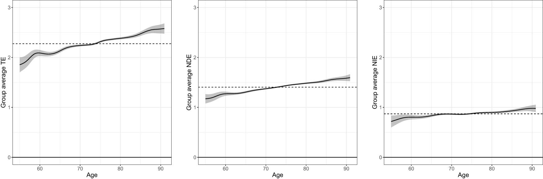
Effects heterogeneity regarding age, where “Group average TE (NDE, NIE)” means estimate of

Effects heterogeneity regarding education level, where “Group average (NDE, NIE)” means estimate of
We find effect heterogeneity related to age manifested by all the causal pathways. As shown in Figure 5, the three kinds of GACEs are all associated with age. The group average NDE (
5.1.5 Best linear prediction of GACEs
Considering that the GACEs presented above are only univariate, we now model GACEs using the multivariate OLS regression with six covariates. Although it may be misspecified, the model gives the best linear predictor of GACEs with six covariates and provides an accessible summary of the effect heterogeneities. As seen in Table 6, the results are basically in accordance with those we obtained earlier. For example, the white coefficient for the group average TE is significant and positive, suggesting that the white group with the APOE-
Coefficients and heteroscedasticity robust standard errors (in parentheses) of best linear prediction of GACEs. *
|
|
|
|
|
|---|---|---|---|
| Constant | 0.697*** (0.065) | 0.359*** (0.054) | 0.338*** (0.064) |
| Age | 0.018*** (0.001) | 0.013*** (0.001) | 0.006*** (0.001) |
| Male |
|
|
0.008 (0.010) |
| Education level |
|
0.003* (0.002) |
|
| Hispanic or Latino |
|
|
|
| White | 0.147*** (0.021) | 0.040** (0.016) | 0.106*** (0.020) |
| Married | 0.157*** (0.012) | 0.055*** (0.010) | 0.102*** (0.011) |
5.2 Average causal effects
It is worth mentioning that, based on the three kinds of estimated ICEs, we can also obtain the average causal effects: average TE =
6 Discussion and conclusion
Machine learning is becoming a powerful tool for precision medicine. In this study, we introduced a novel approach, CGAN-ICMA, to estimate the ICEs and explore the individualized causal mechanism. CGAN-ICMA, composed of two components – the mediator block and the outcome block – does not presuppose the forms of the model and can effectively model complex nonlinear relationships, thus enhancing model flexibility and analytic power. Furthermore, CGAN-ICMA not only estimates average causal effects but also can accurately estimate ICEs. The utility of CGAN-ICMA was evaluated through simulation studies and an application to the ADNI dataset. In the simulation studies, we proposed several metrics to assess CGAN-ICMA and compare it with five other state-of-the-art methods. The results showed that CGAN-ICMA outperformed all others. In the application, we estimated the ICEs of the existence of the APOE-
This study can be extended in several directions. First, CGAN-ICMA can only estimate the ICEs of binary treatment. However, we believe that extending our method to more general types of treatments, including categorical and continuous treatments, would be an interesting problem to explore in the future. This extension can be realized by changing the mathematical formulations of the generator and discriminator for both mediator and outcome blocks. Second, we imposed linear assumption on the mediator–outcome relationship to make it easier to apply the proposed method to multiple-mediator problems. However, in real-world scenarios, the relationship between the outcome and the mediators may be more complex. One promising extension would be to turn to more plausible assumptions and network setups that allow for sampling from the joint distribution of the complete potential mediators, but this may raise theoretical challenges. Nonetheless, our method offers a valuable alternative to existing approaches, particularly for situations where nonlinear relationships are present, but the structure of LSEM may not be suitable. Third, Adam was chosen as the optimizer to train CGAN-ICMA, but it is possible to derive a better optimization algorithm to train our model. In simulation studies, we proposed several metrics to evaluate the empirical performance of CGAN-ICMA. Exploration of richer discrepancy metrics would be interesting future work. Finally, sensitivity analysis is crucial for evaluating the robustness of the obtained causal conclusions toward violation of the unconfoundedness assumption, which is always untestable. Popular strategies developed for parametric mediation models include (1) evaluating certain sensitivity parameters, such as the error correlation between the mediator and outcome models and the proportion of unexplained variance of the outcome that is explained by incorporating treatment–mediator interaction terms [16]; (2) modeling the joint distribution of the potential mediators and potential outcomes, as well as
Supplementary Material
This Supplementary Material includes the pseudo-code of the computer algorithm, the hyperparameters of CGAN-ICMA, additional numerical results, and derivation of equation (6).
Acknowledgments
The authors are thankful to the editor, the associate editor, and two anonymous reviewers for their valuable comments.
-
Funding information: This research was fully supported by GRF Grant (14303622) from Research Grant Council of the Hong Kong Special Administration Region.
-
Author contributions: Cheng Huan is responsible for method development and numerical studies; Rongqian Sun is responsible for method development and preliminary draft; Xinyuan Song is accountable for model establishment, manuscript writing, and revision.
-
Conflict of interest: The authors state no conflict of interest.
-
Ethical approval: The study needs no ethical approval.
-
Informed consent: N.A.
-
Data availability statement: This study generates no new data.
References
[1] Huang YT, Cai T. Mediation analysis for survival data using semiparametric probit models. Biometrics. 2016;72(2):563–74. 10.1111/biom.12445Search in Google Scholar PubMed
[2] Schaid DJ, Sinnwell JP. Penalized models for analysis of multiple mediators. Genetic Epidemiol. 2020;44(5):408–24. 10.1002/gepi.22296Search in Google Scholar PubMed PubMed Central
[3] Sun R, Zhou X, Song X. Bayesian causal mediation analysis with latent mediators and survival outcome. Struct Equ Model Multidiscipl J. 2021;28(5):778–90. 10.1080/10705511.2020.1863154Search in Google Scholar
[4] Zhou X, Song X. Mediation analysis for mixture Cox proportional hazards cure models. Stat Meth Med Res. 2021;30(6):1554–72. 10.1177/09622802211003113Search in Google Scholar PubMed
[5] VanderWeele TJ, Vansteelandt S. Odds ratios for mediation analysis for a dichotomous outcome. Amer J Epidemiol. 2010;172(12):1339–48. 10.1093/aje/kwq332Search in Google Scholar PubMed PubMed Central
[6] VanderWeele T, Vansteelandt S. Mediation analysis with multiple mediators. Epidemiol Meth. 2014;2(1):95–115. 10.1515/em-2012-0010Search in Google Scholar PubMed PubMed Central
[7] MacKinnon DP, Lockwood CM, Hoffman JM, West SG, Sheets V. A comparison of methods to test mediation and other intervening variable effects. Psychol Meth. 2002;7(1):83. 10.1037//1082-989X.7.1.83Search in Google Scholar
[8] Rucker DD, Preacher KJ, Tormala ZL, Petty RE. Mediation analysis in social psychology: Current practices and new recommendations. Social Personality Psychol Compass. 2011;5(6):359–71. 10.1111/j.1751-9004.2011.00355.xSearch in Google Scholar
[9] Shrout PE, Bolger N. Mediation in experimental and nonexperimental studies: new procedures and recommendations. Psychol Methods. 2002;7(4):422. 10.1037//1082-989X.7.4.422Search in Google Scholar
[10] Woodworth RS. Psychology (revised edition). New York: Henry Holt & Co; 1929. Search in Google Scholar
[11] Wright S. The method of path coefficients. Ann Math Stat. 1934;5(3):161–215. 10.1214/aoms/1177732676Search in Google Scholar
[12] MacKinnon DP. Introduction to statistical mediation analysis. New York, NY: Routledge; 2012. 10.4324/9780203809556Search in Google Scholar
[13] VanderWeele T. Explanation in causal inference: methods for mediation and interaction. United States of America: Oxford University Press; 2015. Search in Google Scholar
[14] Huang YT, Yang HI. Causal mediation analysis of survival outcome with multiple mediators. Epidemiology (Cambridge, Mass). 2017;28(3):370. 10.1097/EDE.0000000000000651Search in Google Scholar PubMed PubMed Central
[15] Imai K, Keele L, Tingley D. A general approach to causal mediation analysis. Psychol Methods. 2010;15(4):309. 10.1037/a0020761Search in Google Scholar PubMed
[16] Imai K, Yamamoto T. Identification and sensitivity analysis for multiple causal mechanisms: Revisiting evidence from framing experiments. Political Anal. 2013;21(2):141–71. 10.1093/pan/mps040Search in Google Scholar
[17] Rubin DB. Causal inference using potential outcomes: Design, modeling, decisions. J Amer Stat Assoc. 2005;100(469):322–31. 10.1198/016214504000001880Search in Google Scholar
[18] Cho SH, Huang YT. Mediation analysis with causally ordered mediators using Cox proportional hazards model. Stat Med. 2019;38(9):1566–81. 10.1002/sim.8058Search in Google Scholar PubMed
[19] Lange T, Hansen JV. Direct and indirect effects in a survival context. Epidemiology. 2011;22(4):575–81. 10.1097/EDE.0b013e31821c680cSearch in Google Scholar PubMed
[20] VanderWeele TJ. Causal mediation analysis with survival data. Epidemiology (Cambridge, Mass). 2011;22(4):582. 10.1097/EDE.0b013e31821db37eSearch in Google Scholar PubMed PubMed Central
[21] Tchetgen EJT. On causal mediation analysis with a survival outcome. Int J Biostat. 2011;7(1):0000102202155746791351. 10.2202/1557-4679.1351Search in Google Scholar PubMed PubMed Central
[22] Tchetgen EJT, Shpitser I. Semiparametric theory for causal mediation analysis: efficiency bounds, multiple robustness, and sensitivity analysis. Ann Stat. 2012;40(3):1816. 10.1214/12-AOS990Search in Google Scholar PubMed PubMed Central
[23] Kim C, Daniels MJ, Marcus BH, Roy JA. A framework for Bayesian nonparametric inference for causal effects of mediation. Biometrics. 2017;73(2):401–9. 10.1111/biom.12575Search in Google Scholar PubMed PubMed Central
[24] VanderWeele TJ, Vansteelandt S. Conceptual issues concerning mediation, interventions and composition. Statist Interface. 2009;2(4):457–68. 10.4310/SII.2009.v2.n4.a7Search in Google Scholar
[25] Preacher KJ, Rucker DD, Hayes AF. Addressing moderated mediation hypotheses: Theory, methods, and prescriptions. Multivariate Behav Res. 2007;42(1):185–227. 10.1080/00273170701341316Search in Google Scholar PubMed
[26] Valeri L, VanderWeele TJ. Mediation analysis allowing for exposure-mediator interactions and causal interpretation: theoretical assumptions and implementation with SAS and SPSS macros. Psychological Methods. 2013;18(2):137. 10.1037/a0031034Search in Google Scholar PubMed PubMed Central
[27] Park S, Kaplan D. Bayesian causal mediation analysis for group randomized designs with homogeneous and heterogeneous effects: simulation and case study. Multivariate Behav Res. 2015;50(3):316–33. 10.1080/00273171.2014.1003770Search in Google Scholar PubMed
[28] Qin X, Hong G. A weighting method for assessing between-site heterogeneity in causal mediation mechanism. J Educat Behav Stat. 2017;42(3):308–40. 10.3102/1076998617694879Search in Google Scholar
[29] Rosenbaum PR. Model-based direct adjustment. J Amer Stat Assoc. 1987;82(398):387–94. 10.1080/01621459.1987.10478441Search in Google Scholar
[30] Hong G, Deutsch J, Hill HD. Ratio-of-mediator-probability weighting for causal mediation analysis in the presence of treatment-by-mediator interaction. J Educat Behav Stat. 2015;40(3):307–40. 10.3102/1076998615583902Search in Google Scholar
[31] Dyachenko TL, Allenby GM. Bayesian analysis of heterogeneous mediation. Georgetown McDonough School of Business Research Paper; 2018. p. 2600140. Search in Google Scholar
[32] Xue F, Tang X, Kim G, Koenen KC, Martin CL, Galea S, et al. Heterogeneous mediation analysis on epigenomic PTSD and traumatic stress in a predominantly African American cohort. J Amer Stat Assoc. 2022;(just-accepted):1–36. 10.1080/01621459.2022.2089572Search in Google Scholar PubMed PubMed Central
[33] Qin X, Wang L. Causal moderated mediation analysis: Methods and software. Behav Res Methods. 2023:1–21. 10.3758/s13428-023-02095-4Search in Google Scholar PubMed
[34] Forsyth D, Ponce J. Computer vision: a modern approach. New Jersey: Prentice Hall; 2011. Search in Google Scholar
[35] Chowdhary K. Natural language processing. Fundamentals Artif Intelligence. In: Fundamentals of Artificial Intelligence. New Delhi: Springer; 2020. p. 603–49. 10.1007/978-81-322-3972-7_19.Search in Google Scholar
[36] Chen R, Liu H. Heterogeneous treatment effect estimation through deep learning. 2018. ArXiv Preprint ArXiv:181011010. Search in Google Scholar
[37] Chen P, Dong W, Lu X, Kaymak U, He K, Huang Z. Deep representation learning for individualized treatment effect estimation using electronic health records. J Biomed Informatics. 2019;100:103303. 10.1016/j.jbi.2019.103303Search in Google Scholar PubMed
[38] Chu J, Dong W, Wang J, He K, Huang Z. Treatment effect prediction with adversarial deep learning using electronic health records. BMC Med Inform Decision Making. 2020;20(4):1–14. 10.1186/s12911-020-01151-9Search in Google Scholar PubMed PubMed Central
[39] Ge Q, Huang X, Fang S, Guo S, Liu Y, Lin W, et al. Conditional generative adversarial networks for individualized treatment effect estimation and treatment selection. Frontiers Genetics. 2020;11:585804. 10.3389/fgene.2020.585804Search in Google Scholar PubMed PubMed Central
[40] Yoon J, Jordon J, Van Der Schaar M. GANITE: Estimation of individualized treatment effects using generative adversarial nets. In: International Conference on Learning Representations; 2018. Search in Google Scholar
[41] Apostolova LG, Dutton RA, Dinov ID, Hayashi KM, Toga AW, Cummings JL, et al. Conversion of mild cognitive impairment to Alzheimer disease predicted by hippocampal atrophy maps. Archives Neurol. 2006;63(5):693–9. 10.1001/archneur.63.5.693Search in Google Scholar PubMed
[42] Apostolova LG, Green AE, Babakchanian S, Hwang KS, Chou YY, Toga AW, et al. Hippocampal atrophy and ventricular enlargement in normal aging, mild cognitive impairment and Alzheimer’s disease. Alzheimer Disease Associated Disorders. 2012;26(1):17. 10.1097/WAD.0b013e3182163b62Search in Google Scholar PubMed PubMed Central
[43] Barnes J, Bartlett JW, van de Pol LA, Loy CT, Scahill RI, Frost C, et al. A meta-analysis of hippocampal atrophy rates in Alzheimer’s disease. Neurobiol Aging. 2009;30(11):1711–23. 10.1016/j.neurobiolaging.2008.01.010Search in Google Scholar PubMed PubMed Central
[44] Fox NC, Freeborough PA, Rossor MN. Visualisation and quantification of rates of atrophy in Alzheimeras disease. The Lancet. 1996;348(9020):94–7. 10.1016/S0140-6736(96)05228-2Search in Google Scholar PubMed
[45] Jack CR, Petersen RC, O’brien PC, Tangalos EG. MR-based hippocampal volumetry in the diagnosis of Alzheimeras disease. Neurology. 1992;42(1):183–3. 10.1212/WNL.42.1.183Search in Google Scholar
[46] Thompson PM, Hayashi KM, De Zubicaray GI, Janke AL, Rose SE, Semple J, et al. Mapping hippocampal and ventricular change in Alzheimer disease. Neuroimage. 2004;22(4):1754–66. 10.1016/j.neuroimage.2004.03.040Search in Google Scholar PubMed
[47] Verghese PB, Castellano JM, Holtzman DM. Apolipoprotein E in Alzheimer’s disease and other neurological disorders. Lancet Neurol. 2011;10(3):241–52. 10.1016/S1474-4422(10)70325-2Search in Google Scholar PubMed PubMed Central
[48] Wang W, Nelson S, Albert JM. Estimation of causal mediation effects for a dichotomous outcome in multiple-mediator models using the mediation formula. Statist Med. 2013;32(24):4211–28. 10.1002/sim.5830Search in Google Scholar PubMed PubMed Central
[49] Imbens GW, Rubin DB. Causal Inference in Statistics, Social, and Biomedical Sciences. Cambridge University Press; 2015. 10.1017/CBO9781139025751Search in Google Scholar
[50] Mirza M, Osindero S. Conditional generative adversarial nets. 2014. ArXiv Preprint ArXiv:14111784. Search in Google Scholar
[51] Goodfellow I, Bengio Y, Courville A. Deep learning. Cambridge: MIT Press; 2016. Search in Google Scholar
[52] Kingma DP, Ba J. Adam: A method for stochastic optimization. 2014. ArXiv Preprint ArXiv:14126980. Search in Google Scholar
[53] Seber GA, Lee AJ. Linear regression analysis. Hoboken, New Jersey: John Wiley & Sons; 2012. Search in Google Scholar
[54] Kramer O. K-nearest neighbors. In: Dimensionality reduction with unsupervised nearest neighbors. Springer-Verlag Berlin Heidelberg: Springer; 2013. p. 13–23. 10.1007/978-3-642-38652-7_2Search in Google Scholar
[55] Suthaharan S. Support vector machine. In: Machine learning models and algorithms for big data classification. Springer Science+Business Media New York: Springer; 2016. p. 207–35. 10.1007/978-1-4899-7641-3_9Search in Google Scholar
[56] Batra M, Agrawal R. Comparative analysis of decision tree algorithms. In: Nature inspired computing. Springer Nature Singapore Pte Ltd.: Springer; 2018. p. 31–6. 10.1007/978-981-10-6747-1_4Search in Google Scholar
[57] Breiman L. Random forests. Machine Learn. 2001;45(1):5–32. 10.1023/A:1010933404324Search in Google Scholar
[58] Devanand D, Pradhaban G, Liu X, Khandji A, De Santi S, Segal S, et al. Hippocampal and entorhinal atrophy in mild cognitive impairment: prediction of Alzheimer disease. Neurology. 2007;68(11):828–36. 10.1212/01.wnl.0000256697.20968.d7Search in Google Scholar PubMed
[59] Abrevaya J, Hsu YC, Lieli RP. Estimating conditional average treatment effects. J Business Economic Stat. 2015;33(4):485–505. 10.1080/07350015.2014.975555Search in Google Scholar
[60] Knaus MC. Double machine learning-based programme evaluation under unconfoundedness. Econometrics J. 2022;25(3):602–27. 10.1093/ectj/utac015Search in Google Scholar
[61] Knaus MC, Lechner M, Strittmatter A. Machine learning estimation of heterogeneous causal effects: Empirical monte carlo evidence. Econometrics J. 2021;24(1):134–61. 10.1093/ectj/utaa014Search in Google Scholar
[62] Farrer LA, Cupples LA, Haines JL, Hyman B, Kukull WA, Mayeux R, et al. Effects of age, sex, and ethnicity on the association between apolipoprotein E genotype and Alzheimer disease: a meta-analysis. Jama. 1997;278(16):1349–56. 10.1001/jama.278.16.1349Search in Google Scholar
[63] Tang MX, Stern Y, Marder K, Bell K, Gurland B, Lantigua R, et al. The APOE-ε4 allele and the risk of Alzheimer disease among African Americans, whites, and Hispanics. Jama. 1998;279(10):751–5. 10.1001/jama.279.10.751Search in Google Scholar PubMed
[64] Hayfield T, Racine JS. Nonparametric econometrics: The np package. J Stat Software. 2008;27:1–32. 10.18637/jss.v027.i05Search in Google Scholar
[65] Albert JM, Wang W. Sensitivity analyses for parametric causal mediation effect estimation. Biostatistics. 2015;16(2):339–51. 10.1093/biostatistics/kxu048Search in Google Scholar PubMed PubMed Central
[66] McCandless LC, Somers JM. Bayesian sensitivity analysis for unmeasured confounding in causal mediation analysis. Stat Meth Med Res. 2019;28(2):515–31. 10.1177/0962280217729844Search in Google Scholar PubMed
© 2024 the author(s), published by De Gruyter
This work is licensed under the Creative Commons Attribution 4.0 International License.
Articles in the same Issue
- Research Articles
- Evaluating Boolean relationships in Configurational Comparative Methods
- Doubly weighted M-estimation for nonrandom assignment and missing outcomes
- Regression(s) discontinuity: Using bootstrap aggregation to yield estimates of RD treatment effects
- Energy balancing of covariate distributions
- A phenomenological account for causality in terms of elementary actions
- Nonparametric estimation of conditional incremental effects
- Conditional generative adversarial networks for individualized causal mediation analysis
- Mediation analyses for the effect of antibodies in vaccination
- Sharp bounds for causal effects based on Ding and VanderWeele's sensitivity parameters
- Detecting treatment interference under K-nearest-neighbors interference
- Bias formulas for violations of proximal identification assumptions in a linear structural equation model
- Current philosophical perspectives on drug approval in the real world
- Foundations of causal discovery on groups of variables
- Improved sensitivity bounds for mediation under unmeasured mediator–outcome confounding
- Potential outcomes and decision-theoretic foundations for statistical causality: Response to Richardson and Robins
- Quantifying the quality of configurational causal models
- Design-based RCT estimators and central limit theorems for baseline subgroup and related analyses
- An optimal transport approach to estimating causal effects via nonlinear difference-in-differences
- Estimation of network treatment effects with non-ignorable missing confounders
- Double machine learning and design in batch adaptive experiments
- The functional average treatment effect
- An approach to nonparametric inference on the causal dose–response function
- Review Article
- Comparison of open-source software for producing directed acyclic graphs
- Special Issue on Neyman (1923) and its influences on causal inference
- Optimal allocation of sample size for randomization-based inference from 2K factorial designs
- Direct, indirect, and interaction effects based on principal stratification with a binary mediator
- Interactive identification of individuals with positive treatment effect while controlling false discoveries
- Neyman meets causal machine learning: Experimental evaluation of individualized treatment rules
- From urn models to box models: Making Neyman's (1923) insights accessible
- Prospective and retrospective causal inferences based on the potential outcome framework
- Causal inference with textual data: A quasi-experimental design assessing the association between author metadata and acceptance among ICLR submissions from 2017 to 2022
- Some theoretical foundations for the design and analysis of randomized experiments