Food Crises in Germany, 1500–1871
-
Hakon Albers
Hakon Albers is a post-doctoral researcher at Martin Luther University Halle-Wittenberg, where he received his PhD in economics in 2020. He does quantitative research at the intersection of growth & development, economic history, and agricultural economics. He has analyzed agricultural production and trade in different contexts considering the impacts of climate and weather. Recent key publications are:H. Albers/C. Gornott/S. Hüttel , How Do Inputs and Weather Drive Wheat Yield Volatility? The Example of Germany, in: Food Policy 70, 2017, pp. 50-61; andH. Albers/U. Pfister , Climate Change, Weather Shocks, and Price Convergence in Pre-industrial Germany, in: European Review of Economic History 25, 2021, pp. 467-489. and
Ulrich Pfister
and
Ulrich Pfister
Ulrich Pfister is Senior Professor of Social and Economic History at the University of Münster since 1996. He received his PhD from the University of Zürich in 1984, theHabilitation followed in 1991. His research covers the social and economic history of Europe from the sixteenth to the nineteenth century. He has published in the fields of historical demography, the development of regional export industries, the history of religion, agricultural history and economic growth. Recent publications include:U. Pfister/J.-O. Hesse/M. Spoerer/N. Wolf (eds.) , Deutschland 1871. Die Nationalstaatsbildung und der Weg in die moderne Wirtschaft, Tübingen 2021, english version:U. Pfister/N. Wolf (Eds.) , An Economic History of the First German Unification. State Formation and Economic Development in a European Perspective, London 2023; andU. Pfister , Economic Growth in Germany, 1500–1850, in: Journal of Economic History 82, 2022, pp. 1071-1107.

Abstract
This study is the first to establish a chronology of food crises in Germany from the sixteenth century to their disappearance in the late 1860s based on a standard methodology to detect cycles in commodity prices. To this end, we develop an aggregate rye price series, deflate it by a consumer price index and decompose this real price in trend and cyclical components using the Butterworth filter. Years are classified as food price crisis when the cyclical component exceeds the trend component by 20 percent or more. Using this methodology, we identify 24 food crises between the 1540s and 1871. Additional information from other research is employed to assess the demographic consequences of food price crises. Viewing the latter from an aggregate perspective suggests four distinct regimes of food crises driven by climate change and economic forces.
1 Introduction
This study explores the timing and magnitude of short-term spikes of grain prices in Germany from the sixteenth to the nineteenth centuries. The relevance of this topic stems from two stylized facts about historical economies prior to the onset of modern economic growth and globalization in the nineteenth century. First, because the income of most households was low, expenditure on food dominated household budgets, and grain formed the principal ingredient for most foods, either directly for products such as bread, beer or mush, or indirectly in the form of animal feed. [1] Second, poor harvests resulting from adverse weather conditions could lead to negative shocks in the supply of grain at the regional level. Given a long-term trend of market integration, trade increasingly held the potential to compensate for these regional deficiencies but its contribution to stabilize consumption remained mostly limited to areas along navigable waterways. [2] Furthermore, some crop failures transcended the regional level. Thus, poor harvests that entailed high grain prices could lead to economic crises and famines that took a heavy toll on human lives, sometimes on a pan-European scale. [3]
With respect to pre-industrial Germany, the short-term dynamics of grain prices and famines more generally remain little studied. To be sure, Hans-Heinrich Bass has developed a detailed chronology and geography of food crises in Prussia during the first half of the nineteenth century, and in an overview, Dominik Collet and Daniel Krämer have presented a chronology of famines from the fourteenth to the early nineteenth centuries. [4] However, their list is based on qualitative accounts of the existing literature concerning individual crises rather than a comparative methodology. There are also a number of valuable monographs on individual food crises or specific regions. [5] However, we still lack a chronology of food crises during the pre-unification era that is based on a unified methodology. Consequently, there is also no research addressing the question of how the pattern of food crises has changed over time.
Based on a quantitative approach, we establish a new chronology of food crises from the sixteenth to the nineteenth centuries and identify a sequence of four crisis regimes over this period. Specifically, we construct aggregate series of real rye prices and apply the Butterworth filter to decompose the price series into trend and cyclical components. Years in which the cyclical component exceeds the trend value of the aggregate price by more than 20 percent are defined as food price crises (from the consumers’ perspective). Based on this method, we identify 24 dearth episodes between the 1540s and 1871, combine them with other data such as vital rates whenever possible, and contextualize these crises with the literature on individual famines or specific regions. This empirical analysis shows that the frequency and severity of food crises evolved in four distinct regimes until food crises disappeared in the late 1860s. To be sure, food crises occurred in the context of the two World Wars, particularly during the winter months of 1916/1917 and 1946/1947. [6] Their characteristics and context differ radically from the historical food crises that form the object of the present enquiry; hence, they are outside the focus of our study.
This article is organized as follows: Section 2 presents the concepts that serve to define and characterize food crises. Section 3 describes the construction of the grain price series that we use to identify food crises. Section 4 explains our empirical strategy to isolate crisis years based on price data. Section 5 discusses the trend of the real rye price and provides an account of the 24 food crises identified using the cyclical component of the rye price. Section 6 combines this evidence with other information to characterize four regimes of food crises between the sixteenth century and the 1860s, and is then followed by a conclusion.
2 Conceptual Framework: Dearth, Famine, and Subsistence Crisis
Existing scholarship has discussed food crises under three conceptual headings, namely, dearth or food price crisis, famine, and subsistence crisis. The term dearth relates to episodes of high food prices. It was used in older literature based on the wording of contemporaries (Teuerung) whereas research on more recent periods and from other disciplines uses the term food price crisis to refer to periods of high prices. [7] With nominal income given and an assumed price elasticity of the demand for food of -0.6, high food prices indicate restricted access to food, and thus potential malnutrition among large segments of the population. [8] Accordingly, dearth indicates a food crisis, and existing literature often uses spikes in grain prices, the most important staple food of the preindustrial period in Europe, as a means to identify food crises. [9]
Dearth implies a decline of food intake to a level that has serious consequences for physical wellbeing, but not necessarily death. [10] A famine, by contrast, is characterised by a lack of food that causes increased mortality. [11] Here, it is important to emphasize that the reduction in actual food intake matters independent of its price. However, given the absence of systematic data on actual food consumption for pre-industrial societies, the price of grain in combination with the two assumptions mentioned above (unchanged nominal income, negative price elasticity of demand) remains a useful proxy variable for a reduction in food consumption and thus a food crisis. Nevertheless, it is essential to combine information on food prices and mortality to distinguish a dearth from a famine, albeit this still remains an indirect and second-best approach given the definition of a famine. This is because other variables matter as well, when considering shortfalls of food consumption, such as the availability of income, wealth, food entitlements and the potential of temporary migration to alleviate nutritional distress. [12]
French scholars in particular have emphasized that food shortages impacted on population not only through higher mortality but also via lower fertility. As a result, the term subsistence crisis (crise de subsistence) entered the literature. [13] The temporary decline of the birth rate distinguishes subsistence crises from other demographic crises, such as epidemics, which need not be related to food crises. Since the population loss resulting from an epidemic ceteris paribus increases the real wage in a Malthusian regime, we would not expect it to go together with a decline in fertility, unless there is an additional negative economic shock such as a harvest failure.
The difference between the concepts of famine and subsistence crisis remains elusive. In both types of crisis, food prices, birth and death rates behave in the same way. While excess mortality is the prime characteristic of famines, Cormac Ó Gráda points out that present-day famines also come along with low birth rates based on the same mechanisms as subsistence crises. [14] The difference mostly arises from historical context. Famines of the late nineteenth and twentieth centuries are typically not called subsistence crises. Rather, this term is reserved for crises of the pre-industrial era, that is, under the Malthusian growth regime. The reverse is not true, however: food price crises during the pre-industrial era are also often called famines if there is excess mortality. [15]
In summary, we use four terms developed in the interdisciplinary literature on food crises: dearth, food price crisis, famine, and subsistence crisis. Dearth and food price crisis are defined through high food prices, and we use them synonymously. This type of food crisis is not necessarily lethal and evidence on vital rates is important to distinguish dearth from famine. For the time before the 1810s, when Germany was in a Malthusian growth regime, we use the terms famine and subsistence crisis as synonyms, because no difference exists between both terms except for the historical context: a subsistence crisis is a famine in a Malthusian setting. [16]
We now review how food shortages can impact on fertility and mortality. Food shortages impacted on population via lower fertility through multiple channels. On the one hand, malnutrition led to amenorrhea; in addition, reduced libido and the temporal separation of spouses in search for employment and food may also have reduced the number of conceptions. On the other hand, the income decline affecting the majority of the population led to a deferral of marriages and births. [17]
The main view in the literature is that death caused by starvation constitutes only a part of the excess mortality observed during famines and subsistence crises. [18] Nutrition-related death may occur in the form of starvation/marasmus (due to protein and energy deficiency), famine edema/dropsy (due to protein deficiency), and as a result of the consumption of poisoned food. [19] In particular, mould in the form of ergot or fusarium tricinctum contaminated grain, the consumption thereof being potentially lethal. Additionally, ergot poisoning also negatively impacts on fertility. [20] Ergot infections of rye were more likely during cool and wet conditions in spring, because these prolonged the flowering stage. [21]
Nevertheless, it is important to acknowledge that excess mortality in famine years was also caused indirectly by infectious diseases rather than directly through poisoning or insufficient quantities of food, and only some of the epidemic diseases noted during food crises resulted from insufficient nutrition. [22] Other recorded diseases are by and large invariant to nutritional status, but their spread was enhanced by the social dislocation arising from the food deficit. A disease that was often connected with malnutrition is bacillary dysentery. By contrast, a typical disease that is considered as invariant to nutritional status but whose spread was amplified by the social circumstances surrounding subsistence crises is louse-borne typhus. Specifically, both typhus and subsistence crises in Europe occurred together in winter and spring. The reason is that cold weather made people stay indoors, where the disease was easily transmitted via lice. The spread of the disease was further extended by famine conditions, because people would travel to other towns in search for food and work.
3 Data
To identify food price crises, we construct several variants of an aggregate real rye price extending from the early sixteenth century to 1871. We opt for rye prices because rye dominated arable farming during the period studied and because it constituted the most important type of vegetable food for most segments of the population. We draw on a novel dataset of nominal grain prices in grams of silver per litre [23] in 70 cities within the borders of the German Empire of 1871 for which we possess information on grain prices both before and after 1800 (see Figure 1). [24] We compute the aggregate real rye price as the arithmetic mean of the values for individual towns. In the following, we first introduce three alternative sample definitions. Second, we explain how we deflate nominal prices.
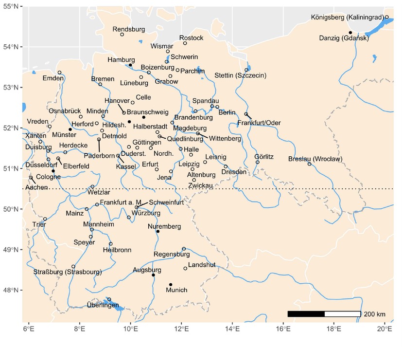
Sample Overview. Note: Black solid circles: stable sample 1561–1860: not more than 5 percent missing observations per individual series. White filled circles: additional cities of unbalanced sample. Abbreviations: Duderst. (Duderstadt), Hildesh. (Hildesheim), Nordh. (Nordhausen). Source: Own representation based on map of Europe from www.naturalearthdata.com. Borders of 1871 from https://hgl.harvard.edu/catalog/harvardghgis1871germanempire (19.10.2024)
We construct three series based on varying sample definitions: The first sample contains all available data points (all 70 cities in Figure 1) with the only restriction that there must be at least five cross-sectional prices in the dataset. This condition is satisfied from 1512 onwards for all years until 1871. Particularly for the first half of the sixteenth century, data are scarce, but from the 1560s onwards, there are always more than ten cities in the dataset; from the 1640s onwards until 1871 coverage exceeds 20 cities. [25] We refer to this sample as our unbalanced sample; it serves to contextualize the other two samples with regard to time and space.
The second sample is what we call the geographically stable sample, in which the number of cities per geographical area is fixed to make the aggregate price comparable across time. In each year, the sample uses five Northern cities and four Southern cities. To allocate cities to Northern and Southern Germany, we split the sample at 50.5° latitude (see dotted line in Figure 1). The sample starts with the earliest available information fulfilling the restriction (in 1543). The inclusion of more than nine cities per year would be beneficial but would also lead to a shorter period covered due to data limitations. Whenever possible the same cities are used; in Table 1 we refer to these cities as main cities. Gaps in each series are filled using the price of the closest replacement city from the same geographical area that is not already part of the sample. For instance, missing years in the series for Hamburg are filled with data from Lüneburg. If a series ends, the same principle applies, that is, Lüneburg substitutes Hamburg. In total, we use information from 23 cities. All cities used in the geographically stable sample and their allocation to the sub-regions are documented in Table 1. [26] Working with a geographically stable sample eliminates the possibility that time variation from additional cities would dominate the variance of the aggregate price.
Cities in the geographically stable sample.
| Northern Germany | Southern Germany | |
|---|---|---|
| Main cities | Braunschweig, Cologne, Gdansk, Hamburg, Xanten | Augsburg, Munich, Nuremberg, Würzburg |
| Replacement cities | Altenburg, Leipzig, Hanover, Dresden, Lüneburg, Vreden, Hildesheim, Celle | Strasbourg, Frankfurt (Main), Speyer, Landshut, Heilbronn, Regensburg |
Source: own representation.
Third, we construct a shorter stable sample with a fixed composition of nine cities with not more than 5 percent missing observations per series (Figure 1, black filled circles). This sample serves as the basis for a consistent high-quality aggregate rye price series that we use as a robustness check on the geographically stable sample.
To distinguish food crises from inflationary shocks and to be able to compare price spikes across time we study the real price, rather than the nominal price of rye. The real price is defined as the price of a particular good divided by the consumer price index (CPI). Prior to 1850, we rely on a CPI based on the value of fixed quantities of eleven goods, which are supposed to reflect the annual consumption of an adult city dweller. In the form of bread, rye also enters this CPI; in the 1760s, the presumed share of bread in total expenditure was 34 percent. However, the price of bread includes a non-negligible labour component (about 20 percent), so that the bread price is less volatile than the price of rye. An increase of the mean rye price by 1 percent was associated with an increase of the CPI by 0.3 percent to 0.4 percent. [27] To obtain a CPI for the whole period under study, we splice this CPI with a CPI based on expenditure shares covering the period 1850–1889 and normalize the resulting index to the year 1701=1. [28] Hence, the real price shown in Figure 2 shows how much ten litres of rye would cost in prices prevailing in 1701. Following Robert Allen’s bread equation and historical evidence, 10 litres of rye correspond to the input necessary to produce 10 pieces of bread with a weight of 0.8 kg each. [29] The year 1701 is chosen to compare these data to the seminal work by Wilhelm Abel on agricultural fluctuations. [30]
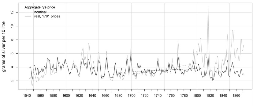
Nominal and real aggregate rye price (real price in 1701 prices). Note: Based on the geographically stable sample. Trend estimated with linear regression for 1701–1800 including dummy variable for the Seven Years’ War (1756–1763). Coefficient for linear trend 1701–1800, real =0.0043, (Newey-West) se = 0.0032, p-value = 0.1898. Coefficient for linear trend 1701–1800, nominal =0.0165, (Newey-West) se = 0.0081, p-value = 0.0447. Data sources: The aggregate nominal rye price is deflated with the consumer price indices from Pfister, The Timing and Pattern, and Pfister, Real Wages, which are spliced in 1850 and normalized to the base year 1701. Grain price data sources: Albers/Pfister, Grain Prices.
Abel studied nominal grain prices and concluded that they increased during most of the eighteenth century. He interpreted this as a result of monetary factors – a renewed influx of precious metals into western Europe – and increased demand resulting from population growth. [31] The nominal rye price in Figure 2 indeed shows a rising trend between about 1701 and 1800 (statistically significant, see note for Figure 2) whereas the real price remained largely stable (trend not significant). Thus, the trend in the nominal rye price was exclusively driven by inflation and was unrelated to real factors such as population growth.
Apart from the eighteenth century, the nominal price increased faster than the real price in the sixteenth and nineteenth centuries. In addition, deflation with the CPI reduces the amplitude of grain price spikes during the Napoleonic Wars (1803–1815) and their aftermath, to a lesser extent also during earlier inflationary episodes related to war finance, such as the so-called Kipper und Wipper era around 1620 and during the Seven Years’ War (1756–1763). [32] These examples show the relevance of the control for inflation for the discussion of grain prices
4 Empirical Strategy
Some authors in famine research and historical demography have used trendcycle decomposition to identify years with high food prices, an avenue we follow here. [33] The tacit assumption of this approach is that the trend is an estimate of what consumers expect about the price level and to which they can adapt. The cyclical component, by contrast, quantifies an unexpected shock.
Econometricians have developed a large portfolio of time series filters. Researchers developing accounts of famines based on prices have employed either a 25-year moving-average (MA) filter or the popular Hodrick-Prescott (HP) filter. [34] In his recent work on the long-term behaviour of commodity prices, David Jacks relies on the Christiano-Fitzgerald (CF) filter and alternatively the Butterworth (BW) filter. [35] We opt for filtering the aggregate price with the BW filter, and run a robustness check with the CF filter (see section 5.3). Appendix A explains our choice of the filter and its specification, most importantly the cut-off frequency.
In line with the existing literature and explorative data analysis, we opt for 20 years as cut-off. That is, cycles with a periodicity of longer than or equal to 20 years (and a frequency lower or equal to 1/20) are part of the trend component; higher frequencies form the cyclical component. In our robustness checks we also vary the cut-off period.
Like Jacks and other literature on commodity prices, we filter the log of the real price. The use of logs is consistent with a log-linear demand function for food consumption in pre-industrial Europe. [36] Thus, the natural logarithm of the real rye price R in year t is decomposed into its trend and cyclical components: log(Rt) = Tt + Ct, where T denotes the trend component and C the cyclical component.
Given that C represents changes in a logarithmic variable, C multiplied by 100 is an approximate percent change. To calculate the exact percentage change, which is relevant for larger deviations during crises, we exponentiate the filtered values: [exp(C) − 1] ∙ 100. [37] This value is used to compare and rank price crises across time. We classify years as food crises when the cyclical component exceeds the trend component by 20 percent or more. From a theoretical perspective, with the demand function mentioned above, which assumes a price elasticity of food demand of -0.6, [38] a surge in the rye price by 20 percent implies a 12 percent reduction in rye consumption, which we consider as substantial. From a statistical perspective, 20 percent is close to the standard deviation (0.198) of log(Rt), which corresponds to 21.9 percent. Assuming a normal distribution for log(Rt), and a trend value at the sample mean, 15.4 percent of the values can be expected to be above this threshold. [39]
To assess the severity of a food crisis, we consider both the deviation from the trend and the duration of a crisis. The latter criterion is motivated by previous studies that observed harvest shortfalls over a number of years aggravating a food crisis. [40] This phenomenon in turn can be related to consumption smoothing, which refers to the behaviour of households to postpone consumption into the future through savings or to bring consumption into the present by liquidating inventories to achieve stable consumption across time. [41] The cost of shifting consumption of the same good (in this case grain) to the future typically depends on the interest rate in the economy, which may be regarded as constant. If households demand more than one good, relative prices matter as well. A higher relative price of grain in a given period makes it relatively more expensive to save grain for future consumption compared to other non-grain goods and thereby reduces savings of grain for follow-up years. Hence, the potential demographic impact of the second or third year of a crisis that extends over multiple years is likely to be more severe than the impact of the first year.
Consumption smoothing implies that the pre-crisis year also needs to be considered to assess the severity of a crisis: A pre-crisis year with a bumper harvest (and a lower relative price of grain than expected) allows consumers to store grain for future crisis years. Furthermore, food consumption in the precrisis year is relatively higher, so that consumers are in comparatively good health at the beginning of the crisis.
Based on these premises, we construct a crisis index that is defined as the sum of price deviations from the trend during all crisis years and the pre-crisis year. A negative deviation from trend in the pre-crisis year reduces the severity of the crisis and vice versa.
One limitation of the approach of detecting crisis years by means of trendcycle decomposition remains: This is a concept of crisis based on relative price changes, whereas the absolute caloric intake, and the related absolute costs matter during famines. Thus, the severity of a crisis that is generated by a combination of high price levels, which go together with a low level of real household income and only comparably small price shocks, might be underestimated.
Nevertheless, giving up the filtering procedure and instead fixing the point of reference simply to the long-term average would neglect the capacity of households to adapt to a changing economic environment: households adjust their consumption choices over time (consumption smoothing) and across goods (responding to relative price changes) as well as their fertility decisions to both food price shocks and trends. [42]
5 The Long-Term Trend of the Real Rye Price and 24 Food Crises
This section presents and discusses the results of the trend-cycle decomposition of the aggregate real rye price from 1512 to 1871. The presentation comes in two parts. Because the identification of food crises depends crucially on the elimination ofthe trend, section 5.1 begins with an interpretation of the trend of the real rye price. Section 5.2 develops a chronology of food price crises at the aggregate level and examines to what extent these crises can be traced in demographic data, while section 5.3 describes robustness checks.
5.1 The Trend of the Real Rye Price
Panel (a) of Figure 3 presents the three versions of the aggregate real rye price for Germany from about 1500 to 1871. All values are in natural logarithms. Panel (b) shows the trend component of the real rye price identified using the BW filter for all three samples over the same period. Panel (a) establishes that the price based on the smaller but geographically stable sample closely follows the overall movement of the larger but heterogeneous unbalanced sample that includes all 70 cities. Similarly, the price based on the geographically stable sample is mostly well in line with the one based on the stable sample of cities with 5 percent or less missing observations but shorter time coverage. This buttresses our confidence that the geographically stable sample represents a good compromise between data coverage and quality. Below, we therefore focus on the geographically stable sample.
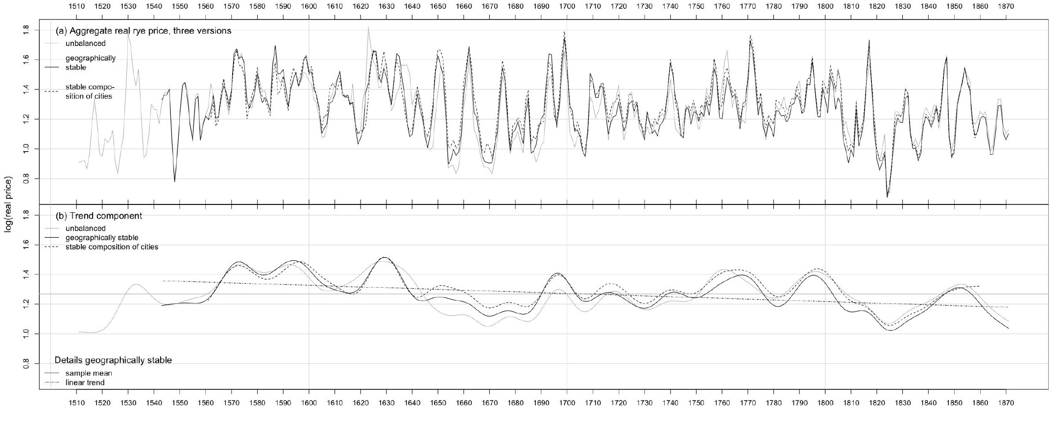
Three versions of the aggregate real rye price and corresponding trend components, Germany, 1512–1871. Note: Panel (a): natural logarithm of aggregate real rye price for three samples: unbalanced sample: 70 cities, varying data coverage; geographically stable sample: 9 cities from 2 geographically fixed areas (Northern and Southern Germany); stable sample: 9 cities with not more than 5 percent missing observations. Panel (b) Trend components from Butterworth filter (Pollock, Trend Estimation), with cut-off frequency 1/20 and order 4. Mean and trend from linear regression shown for geographically stable sample. Data sources: same as Fig. 2.
The trend component displayed in panel (b) indicates changes in the relative scarcity of grain. With a given level of technology, the mid-term movements of the trend component are driven by shifts in relative prices between land-intensive and labour-intensive products. This is because grain is a land-intensive product, whereas the CPI used for deflation also includes products with a considerable labour component, such as linen cloth and beer. Hence, in a Malthusian economy with little technological progress, the trend of the real rye price should parallel swings in population size: Population growth increases the scarcity of land relative to labour; hence, the price of land-intensive products should increase relative to labour-intensive products. By contrast, demographic contraction should produce a decline of the real price. [43]
In the sixteenth and the eighteenth centuries, German population increased by an annual rate of about 0.4 percent and declined by at least a third in the second quarter of the seventeenth century. In 1816–1870 the rate of demographic expansion doubled to 0.8 percent. [44] Following the hypothesis stated above, the real and relative prices of grain should fall in the era of the Thirty Years’ War and should increase during the remainder of the period under study. According to panel (b) of Figure 3, the mid-term movements in the trend of the real price of rye conforms to the expected pattern until the late seventeenth century: the real price of rye rose during the sixteenth century, declined between about 1630 and 1670 and recovered until the end of the seventeenth century. This pattern warrants characterizing Germany as a Malthusian economy during the first two centuries of the modern era.
The situation changed around 1700: Apart from two mid-term peaks in the 1760s and the 1790s and the dip during the agricultural price depression of the 1820s, the trend component of the real rye price remained essentially stable until the end of the period studied, which contradicts the Malthusian hypothesis. If anything, the trend was slightly downward after 1800 despite the acceleration of population growth mentioned above. A linear time trend fitted to the logarithm of the real price based on the geographically stable sample shows that it declined with an annual rate of 0.05 percent per year (p<0.05, Figure 3, panel (b), dot-dashed line). Also, after 1700 the mid-term peaks of the trend component do not reach the high levels prevailing during the sixteenth and seventeenth centuries.
Two factors account for the increased stability of the level of the trend component after 1700: the price of energy and increasing agricultural productivity. First, energy has a considerable weight in the consumer basket underlying the CPI – 11.0 percent in the 1760s, with firewood or charcoal alone making up for 5.5 percent [45] – and the relative price of firewood to rye began to increase continuously from about 1700. This reflects a rising energy intensity of economic growth related to the expansion of proto-industrial iron manufacture and other non-agricultural activities. [46]
Second, the textiles-rye price ratio remained more or less stable between about 1700 and the 1830s. [47] The most obvious explanation is that agricultural supply broadly kept pace with the expanding population. Estimates of grain production in two proto-industrial regions reaching back to the 1730s suggest that this was indeed the case. [48] One potential reason for the expansion of grain output was the advance in grain market integration during the late seventeenth and early eighteenth centuries. [49] The resulting reduction of trade costs must have improved the efficiency of the allocation of factors of production. The behaviour of the real rye price thus establishes that Malthusian forces began to lose sway over Germany from about 1700. This conclusion departs from earlier research by Wilhelm Abel who posited that Malthusian forces continued to prevail until the middle of the nineteenth century. [50]
5.2 A Chronology of Food Price Crises
Panel (a) of Figure 4 again shows the logarithm of the real rye price for the geographically stable sample from 1543 to 1871. Panel (b) shows the cyclical component of the real rye price both for the geographically stable sample and the sample with a fixed composition of cities (the stable sample). Our discussion again focuses on the results for the geographically stable sample and uses the information on the stable sample as a cross-check. The peaks of the cyclical component of the geographically stable sample (marked with vertical bars and corresponding years at the bottom of panel (a) in Figure 4) indicate food price crises (when the cyclical component of the real price exceeds the trend by at least 20 percent). We regard contiguous years with high prices as one single crisis.
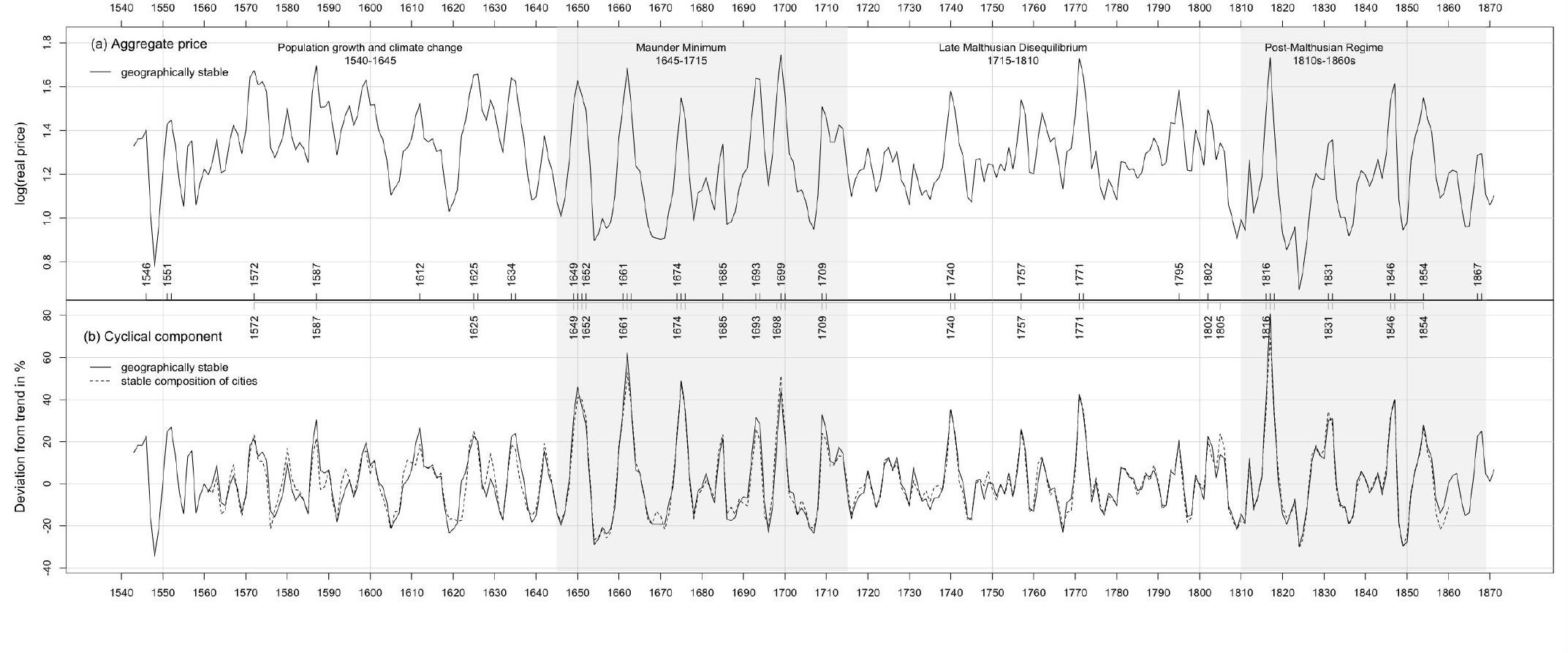
Aggregate real rye price and food price crises in Germany, 1543–1871. Note: Panel (a) plots the natural logarithm of the aggregate real rye price for the geographically stable sample. Vertical lines and years indicated on the horizontal axis in panel (a) mark major price peaks (cyclical component exceeds trend component by at least 20 percent). The grey upper horizontal axis in panel (b) and corresponding crisis years refers to our robustness check using the rye price based on the stable sample. Data sources: same as in Figure 2.
We find 24 price crises within the period studied based on the geographically stable sample with a total of 44 crisis years; 15 of these crises are multiyear crises. Table 2 presents an overview of all food price crises in chronological order. Columns 2 and 3 show the years in which the individual crisis began and ended, column 4 shows the number of corresponding crisis years and column 5 the year within the crisis period in which the rye price reached a peak. Columns 6 to 8 show the percentage deviation from the trend in the pre-crisis year, the first crisis year and in the peak year, respectively. In addition, column 9 presents the cumulative percentage deviation from the trend over the whole crisis period including the pre-crisis year. In column 10 we rank all crises based on this criterion. To classify the crises as dearth, famine or subsistence crises, we also include demographic data if available (columns 11 to 14).
Years of dearth based on cyclical component of aggregate real rye price.
| (1) | (2) | (3) | (4) | (5) | (6) | (7) | (8) | (9) | (10) | (11) | (12) | (13) | (14) |
|---|---|---|---|---|---|---|---|---|---|---|---|---|---|
| Crisis no. | start year | end year | no. of years within crisis | year of price peak | cyclical component in pre-crisis year (%) | cyclical component in first year (%) | peak deviation (%) | sum of deviations (%) | crisis rank sum | CDR, sum cyclical component (%) | CBR, sum cyclical component (%) | burials South, sum cyclical component (%) | baptisms South, sum cyclical component (%) |
| 1 | 1546 | 1546 | 1 | 1 | 18.2 | 22.7 | 22.7 | 40.8 | 19 | ||||
| 2 | 1551 | 1552 | 2 | 2 | 0.9 | 24.7 | 26.9 | 52.4 | 12 | ||||
| 3 | 1572 | 1572 | 1 | 1 | 18.5 | 21.1 | 21.1 | 39.6 | 20 | ||||
| 4 | 1587 | 1587 | 1 | 1 | 16.8 | 30.4 | 30.4 | 47.2 | 15 | ||||
| 5 | 1612 | 1612 | 1 | 1 | 19.2 | 26.5 | 26.5 | 45.8 | 17 | ||||
| 6 | 1625 | 1626 | 2 | 1 | 15.9 | 22.6 | 22.6 | 58.6 | 11 | ||||
| 7 | 1634 | 1635 | 2 | 2 | 1.5 | 22.2 | 23.9 | 47.6 | 14 | ||||
| 8 | 1649 | 1652 | 4 | 2 | 2.6 | 31.4 | 46.0 | 144.8 | 3 | ||||
| 9 | 1661 | 1663 | 3 | 2 | 16.3 | 36.5 | 62.2 | 151.3 | 2 | ||||
| 10 | 1674 | 1676 | 3 | 2 | -1.8 | 23.0 | 49.0 | 104.8 | 4 | 51.9 | -79.5 | ||
| 11 | 1685 | 1685 | 1 | 1 | 11.1 | 21.6 | 21.6 | 32.7 | 21 | -30.5 | 33.0 | ||
| 12 | 1693 | 1694 | 2 | 1 | 13.4 | 31.6 | 31.6 | 73.0 | 9 | 49.3 | -47.2 | ||
| 13 | 1699 | 1700 | 2 | 1 | 17.8 | 44.0 | 44.0 | 84.5 | 5 | 5.1 | 25.3 | ||
| 14 | 1709 | 1710 | 2 | 1 | -11.0 | 32.7 | 32.7 | 46.9 | 16 | 14.1 | -3.0 | ||
| 15 | 1740 | 1741 | 2 | 1 | 14.4 | 35.1 | 35.1 | 73.6 | 8 | 23.0 | -11.0 | 5.S | -7.5 |
| 16 | 1757 | 1757 | 1 | 1 | 5.0 | 25.9 | 25.9 | 30.9 | 22 | 32.6 | -16.9 | 29.0 | -3.8 |
| 17 | 1771 | 1772 | 2 | 1 | 8.2 | 42.3 | 42.3 | 83.3 | 6 | 63.8 | -28.2 | 53.2 | -19.0 |
| 18 | 1795 | 1795 | 1 | 1 | 4.3 | 20.9 | 20.9 | 25.2 | 23 | 24.3 | -7.8 | 18.1 | -7.5 |
| 19 | 1802 | 1802 | 1 | 1 | -7.4 | 22.5 | 22.5 | 15.0 | 24 | -13.8 | 7.6 | 3.9 | 8.5 |
| 20 | 1816 | 1818 | 3 | 2 | 3.4 | 39.8 | 80.9 | 156.0 | 1 | 0.7 | -3.6 | 0.4 | -27.8 |
| 21 | 1831 | 1832 | 2 | 2 | 11.9 | 30.1 | 30.9 | 72.8 | 10 | 6.7 | -6.7 | 3.6 | 0.4 |
| 22 | 1846 | 1847 | 2 | 2 | 4.9 | 31.5 | 40.0 | 76.4 | 7 | 10.3 | -12.5 | 1.8 | -18.7 |
| 23 | 1854 | 1854 | 1 | 1 | 13.9 | 28.0 | 28.0 | 41.9 | 18 | 4.5 | -11.9 | ||
| 24 | 1867 | 1868 | 2 | 2 | 2.5 | 22.6 | 24.9 | 49.9 | 13 | -6.1 | -6.7 |
Note: own calculations. Cyclical components from Butterworth filter as in Figure 4. The sum of cyclical components in vital events includes the first post-crisis year. Aggregate price based on geographically stable sample. Data sources: same as in Figure 2; additional demographic data from U. Pfister/G. Fertig, The Population History of Germany. Research Strategy and Preliminary Results, MPIDR Worming Papers No. 2010-035, Max-Planck-Institute for Demographic Research, 2010 (for numbers of burials and baptism in South Germany); Pfister/Fertig, From Malthusian Disequilibrium, Online appendix (CDR Crude Death Rate, CBR Crude Birth Rate at aggregate level from 1730).
While large and long-lasting deviations from the trend are informative about the level of economic stress, we would like to know more about these crises: were they part of European-wide shocks? What do we know about their demographic impact? Hence, we contextualize all 24 crises using information from the current historiography on local, regional, national, and European crises. To this end, we use the overview by Guido Alfani and Cormac Ó’ Gráda, who develop a European chronology of famines based on the criteria of high grain prices and high mortality in which at least two of nine macro-regions of the continent were affected. [51] The chapter by Dominik Collet and Daniel Krämer on Germany, Switzerland and Austria in the same volume serves as our benchmark at the country level. [52] The quantitative approach of our study complements these overviews in two ways. First, we date and rank crises within a unified methodological framework and discover hitherto unknown food price crises. Second, we draw on vital rates from recent historical demographic work to check whether food price crises also qualify as subsistence crises. [53]
While Collet and Krämer also discuss evidence on famines dating back until the fourteenth century, [54] our crisis chronology starts only in the middle of the sixteenth century due to data limitations. Visual evidence from the unbalanced sample in Figure 3 in Section 5.1 suggests that there certainly was a major food crisis in the first half of the 1530s. [55] Figure 3 also suggests a likely strong earlier shock in 1517. [56] We do not include these two crises in our chronology, because the geographically stable sample does not cover these years.
Whenever possible, we complement our discussion of individual crises with information on local and regional events in Germany, which is mostly based on local prices as well as demographic data where available. In a few cases, output data (tithe or yields) are available as an additional indicator of yield quantity; low yield quality is traced with information on ergot poisoning, medical descriptions of which surfaced in the late sixteenth century. [57] Similarly, we list three crises that do not feature in our baseline result but are mentioned in the existing literature.
The first two food crises we identify when using our methodology occurred in 1546 and 1551/1552. Neither of them has been documented in the existing literature, but the second price crisis coincides with a marked downturn of tithe returns, which proxy grain output, around Nuremberg. [58] The first major famine in our chronology that is covered by the existing literature is the one of the early 1570s. [59] The cyclical component of the real rye price in 1572 is relatively small, but note that the trend component experienced a massive rise around 1570 (Figure 3). During several years of the 1570s, the trend component as such is more than 20 percent above the long-term mean shown in Figure 3, panel (b). There were only three such episodes in the entire period of observation. [60] Thus, our analysis suggests that the severity of this crisis, which is attested by qualitative accounts, resulted from the combination of forces operating in the medium term and short-term shocks. The price crisis of 1587 was a European crisis but has not been documented for Germany yet. There is regional evidence for an ergot epidemic in Silesia in 1587, and there was considerable excess mortality in Nuremberg, albeit slightly earlier in 1585/1586. Evidence from both regions is consistent with low food availability around this time. [61]
The end of the sixteenth century most likely witnessed a low level of food security. The 1590s saw the second episode in which the trend component was 20 percent above the long-term mean over several years. The real rye price rose almost continuously, culminating in a peak in 1599, which falls only slightly short of the criterion of 20 percent excess above trend (19.6 percent), and is thus not included in Table 2. In our alternative chronology based on the CF filter, the deviation is slightly larger than 20 percent, but when using the sample with a fixed composition of cities, 1599 is again just below the threshold (see below, section 5.3, and Figures 4 and B1). For 1595/1596 ergot epidemics are documented in eight regions, which suggests a severe famine. Low food availability at the end of the sixteenth century is also rendered plausible by below average yields in Franconia, and moderate excess mortality recorded for Nuremberg in 1599/1600. [62]
The price spike of 1612 does not appear in existing chronologies of food crises. Nevertheless, narrative evidence for Ulm (northern Swabia) documents consecutive years with cold winters during the first half of the 1610s, notably in 1611/1612, leading to a shortage in grain. In 1611 and 1614 public authorities distributed grain at a reduced price to the inhabitants of the town. The food crisis followed a plague epidemic peaking in 1611, which may have disrupted the production and distribution of food more severely than it reduced demand. [63] The crises of 1625/1626 and 1634/1635 have been described on the basis of local data on prices, tithes, and mortality for Nuremberg and central Franconia (specifically for 1625–1628, and 1632–1635). Both crises again coincided with massive plague epidemics, which may have adversely affected food supply. The food crisis in the 1620s has been noted at the European level, whereas the one in the 1630s may have been confined to Germany. [64]
Existing chronologies also mention a food crisis in 1620–1623, which does not feature in our results. [65] While European annual, summer, and winter temperatures were far below average at this time (mean -1.5 standard deviations, SD), these years do not belong to the coldest recorded (mean -2 SD). [66] This was, however, also a period of severe currency debasement related to inflationary war financing during the initial stage of the Thirty Years’ War, the so-called Kipper und Wipper era. Whereas nominal prices of all products quoted in debased currency soared during the half decade preceding 1623, the real price of rye was actually below trend around 1620 (see Figure 4, panel (b)). This may reflect an effect of the inflation tax that shifted purchasing power from workers, whose nominal wages remained sticky, to warring rulers and thereby reduced demand for food. Thus, the Kipper und Wipper era likely was a serious economic crisis, but it was not triggered by an adverse supply shock in agriculture that is characteristic of a food crisis. [67]
The crises of 1649-1652 and 1661-1663 have been noted by several studies and are ranked third and second in severity among all 24 crises (column 10 in Table 2). [68] Both crises show cumulative sums of deviation from trend of more than 140 percent and stretch over three and four years, respectively. Regional evidence confirms the severity of these food crises. Specifically, widespread ergot poisoning was reported for the Vogtland (Saxony) in 1648/1649. [69] In Brandenburg and its western possessions, a poor harvest led to a ban on grain exports in 1651, and similar measures were taken in 1660–1662. [70]
The crisis of 1674–1676 was of similar magnitude according to our ranking criterion (see column 10 in Table 2). Its severity is confirmed by evidence from demographic data, which is available from 1675 onwards. We show a cumulative deviation from trend established using the BW filter of the logarithm of the series (specification and calculation of percentage deviation as for the real rye price) during periods of crisis and the first post-crisis year (in columns 11 to 14 in Table 2). Research suggests that vital events reacted both immediately and with a time lag on fluctuations of material living conditions. [71] Thus, we measure the demographic impact of a food crisis with the sum of the deviation from trend in crisis years and one year later. During the crisis of 1674–1676, a sample of parishes located in Southern Germany recorded exceptionally high numbers of deaths and a dip in the number of births. There was also renewed ergot poisoning in Vogtland and Westphalia in 1675. [72] Thus, the grain price spike of 1674–76 clearly qualifies as a subsistence crisis.
The crisis of 1685 features a comparably small deviation from trend (just above 20 percent) and lasted only one year. Evidence concerning vital events in Southern Germany is not consistent with a subsistence crisis. Consequently, 1685 may be best characterized as a dearth episode. By contrast, the crisis of the early 1690s is known as one of the most severe famines in early modern Europe. It is clearly visible in a spike of the number of deaths and a low number of births in a sample of southern German parishes. [73] The crisis of 1699/1700 has been described for Brandenburg-Prussia, North-Western Germany and Saxony. There is also testimony of widespread ergot poisoning in Thuringia in 1699. Given the massive spike in the aggregate rye price (rank 5 according to column 10 of Table 2), this crisis may have been more severe than the crisis of 1693/94 according to the cumulative deviation from trend. While it is not visible in the vital events series based on parishes in Southern Germany, a tentative estimate of vital rates at the aggregate level suggests a spike in the death rate and a trough in the birth rate in 1699, which clearly characterizes this episode as a subsistence crisis. [74]
The food crisis of 1709 has been documented using qualitative evidence for Brandenburg-Prussia, and its demographic effects are reflected in a high number of deaths in 1709/1710 and a low number of births in 1710 in Southern Germany. It has also been characterized as a European-wide crisis but its impact on mortality was weaker compared to the crisis of the early 1690s in most countries. [75]
Dominik Collet and Daniel Krämer mention a food crisis in 1724/1725 in their chronology. We find spikes in the real rye price in these years, but the deviations from trend are less than 20 percent (8.9 percent and 12.7 percent, respectively). In a tentative estimate of aggregate vital rates for this period, there is also a minor spike of the death rate and a small dip in the birth rate in 1724, which combine into a negative rate of natural increase. Finally, contemporary reports mention widespread ergot poisoning in Silesia, parts of Pomerania and Brandenburg in 1722/1723. All this renders it plausible that at least a minor subsistence crisis occurred around 1724. [76]
The crises of 1740 and 1771/1772 are well-known pan-European food crises. However, the one of the early 1770s was apparently much more severe in Germany than in other parts of the continent. [77] The greater severity of the crisis in 1771/1772 relative to the one of the early 1740s is confirmed by our ranking according to the cumulative deviation from trend (rank 6 vs. 8). The crisis of the early 1770s was also characterized by the highest spike in the crude death rate in the aggregate series of life events starting in 1730, and a marked slump in the crude birth rate, rendering it one of the most serious subsistence crises in German demographic history. By contrast, the price peak in 1757 is less known. Nevertheless, this crisis can be clearly identified by an excess of deaths over births in the aggregate series of vital events.
The price spike in 1795 is the last food supply shock that went together with a massive increase of mortality, which – combined with a slump in fertility – produced an excess of deaths over births at the aggregate level. The one of 1802, by contrast, seems to have been a minor crisis; to our knowledge it is mirrored neither in demographic evidence nor in contemporary reports.
From the 1810s to the 1850s, four negative shocks in food supply occurred at short intervals: (i) The first was the crisis of 1816-1818 following the eruption of Mount Tambora in 1815, which resulted in crop failures over consecutive years. [78] This crisis was the most serious one in the period under study with regard to the sum of price deviations from trend (column 10 in Table 2). (ii) The substantial spike in the real price of rye in 1831/1832 does not appear in existing famine chronologies, but deviations of vital events from trend are consistent with a famine, which is corroborated by qualitative evidence for parts of Prussia. [79] (iii) Serious food shortages in 1846/1847 originally arose from the European-wide potato blight spreading from 1845, the effects of which were aggravated by crop failures of cereals in 1846. [80] (iv) The price spike of 1854 was less marked than the one in 1846/1847, which makes this crisis less known, but the mid-term trend of the real rye price shows a massive bulge during the first half of the 1850s (see Figure 3). The economic effects of the combination of a high trend level and a short-term shock were likely of similar severity as those of the shock of 1846/1847: In 1855, the birth and marriage rates showed their lowest values in the entire period between 1815 and 1913, and emigration to overseas destinations reached a peak in 1854. There were also reports on widespread ergot poisoning in several regions. Net industrial capital formation was zero in 1855 and strongly negative in 1856, which suggests that the crisis also affected the nonagricultural sectors. [81]
The crisis of 1868 was the last economic crisis that originated from output shortfalls in the agrarian sector. While emigration to overseas destinations shows a local peak in 1868, the effect on vital rates was small at best. The only exception was in the extreme northeast of the country, the Province of East Prussia, which experienced an excess of deaths over births in 1868 and where there was a high number of deaths attributable to ergot poisoning. [82]
The food crises from the late 1810s to the 1860s share the characteristic that their demographic effects were weaker compared to the crises of the eighteenth century. Notably, the cumulative deviation of the death rate from trend never exceeded 10.3 percent, whereas the deviation was always larger than 23 percent in the food crises that occurred between 1740 and 1795. As a result of the weakening of the response of the death rate to food price shocks, there was no year with a negative rate of natural increase – that is, an excess of deaths over births – at the aggregate level after 1815. The last year that saw a negative rate of natural increase was 1814. It may have been related to a spike of grain prices in 1812 (cyclical component 12.2 percent), which, however, does not qualify as a food crisis according to our criterion. [83] A weakening of the demographic impact of dearth is also documented at the European level, in particular with respect to the Tambora crisis. [84] Nevertheless, high food prices were still accompanied by a decline in the birth rate (column 12 of Table 2) and, hence, the rate of natural increase, a decline in the marriage rate and, increasingly so, spikes in emigration. There were also substantial regional differences. Regions in north-eastern Germany, where the lower classes depended mostly on employment in agriculture, continued to suffer negative rates of natural increase during the crises of 1831/1832, 1846/1847, 1854, and 1868. [85]
5.3 Robustness Checks
We performed four robustness checks to explore the sensitivity of the chronology of the 24 identified food crises and their relative ranking with regard to sample variation and econometric filter. We derived an alternative chronology using the same BW filter but based on the stable sample (as described in Section 3, see plot of cyclical component and corresponding crisis years on grey axis at the top of panel (b) of Figure 4 in Section 5.2). In this alternative version, only 19 crises are detected. Three crises cannot be detected simply because of the shorter period of observation: 1546, 1551 and 1867. Thus, 21 of the 24 crises are left, which are detectable in the stable sample. Three crises do not pass the threshold value and an additional one is detected. The three crises that are missing when using this alternative sample are the ones of 1612, 1634/1635, and 1795. The crisis of 1612 is ranked 17 of 24 in the baseline results; 1634/1635 is a multi-year crisis and has rank 14. In the stable sample the cyclical components for these years are below the threshold value (18.9 percent and 16.3 percent) but still considerably large. In the baseline specification, the deviation from trend in 1795 is just above the threshold of 20 percent and ranked 23; the value based on the stable sample fails to meet this criterion only slightly (19.9 percent). The additional crisis detected with this sample is 1805, lasting one year with a peak of 23.8 percent; the deviation in the geographically stable sample is only 13.8 percent. 1805 was marked by a negative deviation of average temperature, [86] but the demographic response to the crisis was weak and ambiguous. While fertility at the aggregate level deviated negatively from trend in 1805-1806 (-2.8 percent), the death rate also decreased (-4.7 percent). Thus, there was no excess mortality, which contradicts the typical pattern during famines.
The ranking of the top half of the 24 crises changes only slightly (see Table B1 in the Appendix). The most notable change is that the crises of 1685 and 1854 are ranked higher (12 vs. 21 in baseline and 11 vs. 18 in baseline, respectively); by contrast, the one of 1693 has a lower rank (14 vs. 9 in baseline).
Our crisis chronology is also robust when altering the method of time series decomposition to the CF filter. Using this filter, only 23 crises are identified; we show them in the appendix (see Figure B1 and Table B1, Appendix B). The crises that are missing compared to the results based on the BW filter are those in 1546 (at the beginning/end of the sample the CF filter might be unreliable), [87] and 1795 (which is just below the threshold of 20 percent). The year 1599 is an additional crisis year (just above the threshold, see Section 5.2 for a discussion of the historical evidence). There are two minor changes regarding the dating of crises: 1634/1635 is reduced to a single-year crisis (1635), and the crisis of 1674–1676 starts one year later in 1675. The ranking of crises is very similar (see Table B1, Appendix B). Among the top three crises, 1816 and 1661 swap positions. Among the less severe crises, 1551 is now ranked 13 (vs. 12 in baseline) while 1709 is attributed rank 12 (vs. 16 in baseline).
Next to varying the sample and the type of filter, we considered two alternative cut-off periods for the BW filter, P=30, and 60, respectively. Intuitively, a shorter cut-off period attributes more fluctuations to the trend component whereas a longer cut-off period generates a smoother trend (see also Figures B2 and B3, Appendix B). When there are runs of years with high prices, a smoother trend would make it easier to identify a multi-year crisis, because the decomposition attributes less variation to the trend and more to the cyclical component.
The majority of crises is insensitive to these variations; nevertheless, the following modifications appear: The detection of crisis years at the sample end points is different (1540s, 1860s), but in a rather unsystematic way. With a higher cut-off period (P=30, P=60), 1685 (ranked 21 in the baseline) is not a crisis year anymore. More importantly, the crisis of the early 1570s grows in significance as specifications with longer cut-off periods show a higher number of crisis years. In the specification with P=60, 1571–1574 is ranked at 6. In addition, the year 1599 is detected. These results are in line with the strongly rising trend component of the baseline results discussed in Section 5.2 above; with a higher cut-off period more of the variation is attributed to the cyclical component.
These alternative results also make it clear that the importance of the absolute price level is downplayed by trend-cycle decomposition in general. A smoother trend at a longer cut-off period shows a lower level during the 1570s and 1590s, so that the shock (the cyclical component) grows in size, which partly remedies this issue. However, with P=30 the trend level is underestimated at the beginning of the sample when compared to the long-run sample, giving an implausibly high weight to the crisis of the 1540s (see Figures 3 and B2). Furthermore, at higher cut-off periods such as P=60, it also becomes more difficult to argue that the cyclical component represents unexpected shocks to which adaptation is more difficult than to the current trend.
We conclude that our chronology of food crises is largely robust to both sample variation and the method applied to identify cycles in the aggregate real rye price.
6 Four Regimes of Food Crises
To some extent, food crises were the effect of short-term random weather shocks. Nevertheless, the characteristics of food crises were also influenced over longer periods by climate change: temperature and grain prices exhibit a negative correlation in early modern Europe; therefore, the evolution of the Little Ice Age, which culminated between c. 1570 and 1710, should have impacted on grain price fluctuations. [88] Moreover, the German lands underwent profound societal and economic changes in the period studied, involving processes such as state formation, market integration, and the transition to modern economic growth. [89] These general considerations suggest that food crises and their demographic impact shared common characteristics over longer periods of time. In what follows, we present the systematic features of food crises as a sequence of four distinct food crisis regimes.
6.1 Population Growth and Climate Change (c. 1540–1645): Rising Demand Meets Increasingly Constrained Supply
Food crises do not seem to have evolved in any systematic pattern during the sixteenth century with respect to frequency, duration and deviation from trend. However, the trend component of the real rye price experienced a massive rise over time (see Figure 3 and the previous discussion in Section 5): From about 20 percent below the long-term average at the beginning of the century it rose to a level slightly below the mean during the 1540s and 1550s, and peaked at values more than 20 percent above the long-term average in the early 1570s and the 1590s. Thus, whereas the local peaks of the real rye price in 1572, 1587 and 1599 deviated less from trend than the majority of other food crises, the absolute value of the real rye price in those years was at par with the value prevailing in 1642–1652 and 1661–1663, which were years with some of the most serious food price crises according to our ranking. In other words, the food crises of the last three decades of the sixteenth century represent particularly dire episodes in a context where access to food was severely restricted due to very high price levels.
Explanations of the situation in the sixteenth century can be structured by considering the aggregate supply and demand for grain. The first explanation relates to an important supply side factor: climate change. From about 1560 the weather in Central Europe became wetter and colder in all seasons. This increased the likelihood of harvest failures and, correspondingly, of dearth and subsistence crises. The negative relationship between grain prices and temperature implies a structural deterioration in food availability during this period. [90]
The second explanation of the changing behaviour of the real rye price during the sixteenth century relates to the demand side. Between 1500 and 1600, Germany’s population grew by 78 percent from about 7.2 million to about 12.8 million. In line with the textbook model of a Malthusian economy with static technology and a fixed amount of land, the real wage of urban labourers fell by roughly one-half, because population growth reduced the endowment of labour with land. The mid-1590s recorded the lowest level of real wages during the early modern era. Thus, while the real price of rye rose to an extraordinarily high level, income per capita declined; in combination, these two processes reduced the quantity of food that households could demand. [91] Note that population growth may also impact on the supply side: While the amount of land is fixed, not all plots are of the same quality and increasing reliance on marginal land in the wake of the expansion of the cultivated area may have decreased the level of land productivity and increased the variability of harvest outcomes, given that marginal land is more susceptible to shocks. [92]
6.2 The Maunder Minimum (c. 1645–1715): High Frequency and Intensity of Food Price Shocks
The Maunder Minimum (MM) characterizes a climatic period with low solar irradiance, which contributed to low temperatures during the growing season and extremely cold winters. [93] The volatility of the real rye price, measured by the standard deviation of the cyclical component, was 21.7 percent during this period, compared to only 13.6 percent during the preceding phase. The 70 neighbouring years (35 years before and after the MM) feature a volatility of only 12.6 percent. Thus, dearth episodes indicated by rye price spikes were both more frequent and more severe during the MM than before and after. According to Table 2, five of the twelve most severe price crises of the whole modern period occurred during the MM. In addition, the MM exhibits an excess in crisis years: With a total of seven dearth episodes (only 1685 and 1709/1710 do not figure among the twelve most severe crises), this 70-year period contains seventeen crisis years, while the 70 neighbouring years include four dearth episodes with only seven crisis years. Finally, the total cumulative percentage deviation above trend was 638 percent during the MM period, but only 226 percent during the 70 neighbouring years. The demographic evidence that increasingly becomes available from the second half of the seventeenth century qualifies the dearth episodes of this period as subsistence crises except for the crisis of 1685. For this latter case, reports concerning ergot poisoning and export bans provide qualitative evidence of severe restrictions on access to food. The Maunder Minimum period implied that the preceding crises of the 1620s and 1630s, which were aggravated by plague epidemics, were followed by another eighty years of frequent and massive adverse shocks. The mid-seventeenth to early eighteenth century thus presents itself as a prime case of the economic effects of climate change in German economic history.
6.3 The Late Malthusian Disequilibrium (c. 1715 to early 1810s): High Vulnerability to Fewer Shocks
The century preceding 1815 has been characterized as a demographic disequilibrium because of a parallel decline of the death rate and the real wage; there was thus no long-term equilibrium relationship between the real wage and mortality as implied by the Malthusian hypothesis of a positive check. The period also qualifies as late Malthusian because there was still a negative relationship between population and the real wage, whereas other elements of a Malthusian economy had vanished. Recall the early signs of an increase in total factor productivity in agriculture mentioned in Section 5.1. [94] According to the evidence presented in Table 2, rye price crises were less frequent and less severe during this era than both before and after, and price volatility was relatively low (12.2 percent in 1716–1809). However, a salient feature of this period is that while the level of mortality fell, the death rate reacted much more strongly to fluctuations of the real wage than in other European countries at the time. [95] These fluctuations were essentially driven by grain prices. The German population was thus highly vulnerable to adverse shocks in agricultural output. Whereas the frequency and severity of food shortages declined after the end of the Maunder Minimum, they continued to have dire economic consequences and caused immense human suffering; the food crisis of 1771/1772 is a prime example.
6.4 The Post-Malthusian Era (late 1810s to 1860s): High Food Price Volatility Combined with Decreasing Demographic Impact
The period between the late 1810s and the 1860s qualifies as a post-Malthusian era for two reasons: First, the real wage remained stable and there was a progressive increase of the growth rate of real GDP per capita, despite a massive acceleration of population growth. The Malthusian effect of population growth that would dilute the resource endowment of labour was thus fully compensated by forces that raised total factor productivity. Second, as already mentioned above, the death rate was largely insensitive to negative income shocks at the aggregate level; by the late 1810s, the Malthusian positive check had disappeared in a short-term perspective as well. [96] However, during the first part of the post-Malthusian era, rye price volatility surged to 21.2 percent for the years 1810–1859 (19.7 percent for the years 1810-1871), that is, approximately the same level as during the Maunder Minimum period. In less than fifty years, there were four dearth episodes, three of which ranked among the top half of all food crises with respect to our severity indicator (see Tables 2 and B1).
Two explanations stand out to account for the increase in the frequency and magnitude of food price spikes between the late 1810s and the 1860s. The first explanation pertains to climate. Apart from the early 1820s, when weather conditions favoured grain farming (see the negative spike of real rye prices in 1824 in Figure 4), most of the period was characterized by a high frequency of negative temperature anomalies. Conversely, the warming that took place in the 1860s may have contributed to the decline of food price volatility in combination with globalization forces. [97]
A second explanation points to the possibility that third market effects increased grain price volatility between the late 1820s and the onset of the so-called European grain invasion in the 1860s. [98] From the 1760s, the northern parts of Germany had gradually emerged as an important supplier of grain to industrializing Britain. The enactment of the Corn Laws in 1815 temporarily muted this trend, but their progressive dismantling between 1828 and 1846 led to a renewed increase of grain trade between Germany and Britain and to a narrowing of the price gap between English and Prussian grain markets. The rise of the trend component of the real rye price between the 1820s and the 1850s thus reflects an increase in both national and international demand. However, trade volumes were highly volatile: peaks were recorded in 1818, 1830, 1841 and in the late 1840s. [99] Three of these peak years correspond with the food crisis years in our rye price series. This correspondence between food price crises and temporary peaks of grain exports is consistent with views originally presented by George Grantham and Amartya Sen.
Grantham, based on the work of Jean Meuvret, has argued that in a first stage of market integration, when trade costs were still high, long-distance trade of grain was intermittent and largely confined to periods of strong spatially asymmetric shocks. Only when prices were very high in one place and low in another were price gaps large enough to cover trade costs. [100] Sen highlighted the role of demand failure in food crises. [101] In regions where agriculture was the prime source of employment, harvest failures also led to a decline of labour income among the lower class because fewer harvesters and threshers were needed. Because of the decline of local demand, more grain became available for being exported to regions where households depended less on agricultural output for their income. At least at a first glance, the views of Grantham and Sen are consistent with the pattern of food crises during the first part of the post-Malthusian era, that is, high volatilities of grain prices and grain exports as well as the concentration of crisis-related mortality peaks in the north-eastern parts of the Kingdom of Prussia, which had specialized in export-oriented grain production. [102]
However, the question remains: if Prussian export regions were suffering from serious food shortages, why did high food prices no longer lead to a massive increase of mortality at the aggregate level between the late 1810s and 1860s compared to the eighteenth century? Three factors were likely responsible for this phenomenon. First, in contrast to the international level, market integration within Germany may have reduced the occurrence of regional deficiencies in supply much better than before 1815. Market integration was promoted by territorial consolidation and trade reforms during the Napoleonic Wars, the formation of the customs union (Zollverein) in 1834, and infrastructure development like paved roads construction (from the late 1810s) and railways (from the 1840s). [103] Second, the spread of potato cultivation reduced food risk. Potatoes react differently to weather conditions than do cereals, so harvests of rye and potatoes are only moderately correlated. Consequently, the spread of potato cultivation complemented market integration with regard to diversifying sources of food supply. [104] Finally, increasing state capacity and rising per capita income may have increased the volume and efficiency of food aid programmes implemented by both public authorities and private associations. [105]
In Germany, food crises ended in the late 1860s. This end of the historical pattern of food crises in the late 1860s is testified by the complete absence of a mortality response to the food price shock in 1867. Two reasons most likely account for the heightened resilience with respect to adverse shocks in agricultural output around this time. First, the progress of industrialization decreased the dependence of household incomes on agricultural output, which stabilized domestic food demand. Household survey data for industrial workers from 1888/1890 show how industrial incomes contributed to cover the costs of the required nutritional intake. However, German workers still had a low nutritional intake and faced a nutritional gap compared to the USA; consequently, significant welfare gains continued to make emigration attractive. [106]
Second, and notwithstanding rising agricultural protectionism from the 1880s, the globalization of grain markets allowed meeting the food demand of industrial workers through international markets. This is evidenced by the fact that Germany, after having been a net exporter of grain for many years (including the crisis years of the mid-1850s), showed a surplus of grain imports over grain exports in 1867 and 1868; over the following decade, Germany turned from an exporter to an importer of grain around 1870. [107]
7 Conclusion
This study is the first to establish a chronology of food crises in Germany from the sixteenth century to the 1860s based on a standard methodology to detect cycles in commodity prices. To this end, we developed several variants of an aggregate rye price series, deflated it by a consumer price index and decomposed it in trend and cyclical components using the Butterworth filter. The estimated trend stabilized from about 1700 onwards despite rapid population growth, which suggests that Malthusian forces lost their power much earlier than posited by earlier research.
We identify 24 food crises between the 1550s and 1860s, in which the cyclical component exceeds the trend component by 20 percent or more. 15 of these crises extended over multiple years and the three most serious crises (measured by the cumulative deviation from trend during the crises) were in the years 1816, 1661, and 1649.
Viewing all 24 food crises from an aggregate perspective suggests four distinct food crisis regimes driven by climate change and economic forces, which impacted on the extent of price volatility and the vulnerability of demographic variables to price shocks. In the first regime, which lasted from c. 1540 to 1645, population growth resulted in rising demand that faced a constrained supply because of adverse climate change. Whereas this period featured on average high price levels combined with low volatility, the reverse is true for the regime prevailing during the Maunder Minimum (c. 1645–1715). The latter was followed by a late Malthusian disequilibrium that lasted until the early 1810s and featured fewer shocks than the period of the Maunder Minimum, but demographic vulnerability with respect to spikes in food prices was still high. Grain price volatility increased again during the Post-Malthusian era (late 1810s to 1860s) but the demographic impact of food crises at the aggregate level decreased. Among these regimes, the Maunder Minimum stands out with regard to both frequency and severity of food crises. While this is a new result, at least in part this might be related to the applied method, because trend-cycle decomposition focuses on the deviation from trend irrespective of price level, which may downplay the severity of crises during the first regime (characterized by high price levels, low income and comparably small shocks). Unfortunately, we mostly lack the demographic data for the first two regimes to classify the food crises as fullfledged famines with excess mortality; more detailed mortality information could contribute to assess the relative weight of these two regimes.
Future research will have to test econometrically whether the Maunder Minimum regime went hand-in-hand with structural breaks in the behaviour of grain price series. Furthermore, the contrast between the increased amplitude of grain price variations and the weak response of mortality to spikes in the grain prices in the four decades after 1815 calls for further enquiry. Specifically, an indepth analysis of this phenomenon will have to explore the relevance and relative weight of agricultural development, structural change resulting from industrialization, international trade, and the increasing state capacity in accounting for the disappearance of famine-related mortality.
8 Appendix A: Choice and Specification of Filter
Choice of Filter
Earlier research using grain prices to detect food crises applied the MA and the HP filter (cf. section 4). However, both filters have serious disadvantages. The trend estimate from a symmetric MA filter is by construction shorter at both ends of the sample, because leads or lags of the underlying time series are not available. Use of the HP filter has been discouraged by Hamilton. [108]
The CF filter used in the literature on commodity prices is a bandpass filter, that is, it targets a range of frequencies, which pass the filter while the other ones do not. This filter can also be used as a high-pass filter if the minimum period is set to 2. In its baseline version, the CF filter assumes series that are integrated of order 1; nevertheless, it can also be applied to stationary time series. [109] The price series we analyse turn out to be stationary or trend-stationary depending on the specification of the price series and the test chosen (Table A1).
Time series properties of aggregate real rye price.
| Phillips-Perron test | KPSS test | |||||
|---|---|---|---|---|---|---|
| Sample | real | log(real) | real | real | log(real) | log(real) |
| (level) | (trend) | (level) | (trend) | |||
| Unbalanced | <0.01 | <0.01 | >0.1 | 0.0397 | >0.1 | 0.0345 |
| Stable | <0.01 | <0.01 | 0.0246 | >0.1 | 0.023 | >0.1 |
| Geographically stable | <0.01 | <0.01 | <0.01 | >0.1 | <0.01 | >0.1 |
Note: p-values for corresponding tests on real price or logged real price. Type of null hypothesis for Kwiatkowski-Phillips-Schmidt-Shin (KPSS)-test in brackets, e.g., ‘trend’ corresponds to ‘trend stationarity’.
The BW filter developed by Stephen Pollock can be implemented as a low-pass or as a high-pass filter (only low or high frequencies pass the filter); it is applicable to both stationary series and series with a unit root. [110] Thus, both filters can be used to achieve our aim of isolating the cyclical component as an indicator of food crises. Compared to the CF filter, the additional advantage of the BW filter is that it does not alter the frequencies in the passband (the gain of the filter is unity) except around the cut-off frequency. [111]
Specification of the BW Filter
The choice of a periodicity of 20 years is justified on two grounds: previous research and the periodogram of the detrended data. In view of potential longrun cycles, the literature on commodity prices decomposes the latter in three components using the CF filter: a long-run trend with periodicities larger than 70 years, medium-run cycles with a duration of 20 to 70 years, and short-run cycles below 20 years. [112] Medium-run cycles are often driven by demand and are followed by a supply response. In our context, demand for rye would increase with demographic expansion, and the supply response could result from increased specialization (as a result of market integration or learning-by-doing) and/or land expansion. These arguments also answer the question of what drives the long-run trend; the difference between long-run trend and mediumrun cycle is mostly about how long it takes for these structural adjustment processes to unfold. In view of food crises, our aim is to identify the short-run component, not the medium-run cycles.
Furthermore, much lower cut-offs, for example, in the range of three to five years such as used for the analysis of modern business cycles, are at odds with empirical results on pre-industrial grain prices. Spectral analysis of historical rye price series for Germany found cycles with a length of up to 13 and 10 years, respectively. An investigation into European grain prices has established periodicities of 5 and 16 years. [113] The associated price fluctuations should be part of the cyclical component and justify the choice of a longer cut-off periodicity.
In addition, as advised by Pollock, we inspected the periodogram to find frequencies that occur seldom in the data. [114] These frequencies form a natural criterion for the choice of the cut-off frequency of the filter. The periodogram of the linearly detrended natural logarithm of the real price for our preferred sample, the geographically stable sample, exhibits low spectral density between approximately 8 and 21 degrees, see Appendix Figure A1. These values correspond to a period of P=360°/8°=45 years (frequency f=1/45) and P=360°/21°=17.14 years (frequency f=1/17.14). Our cut-off frequency of f=1/20 corresponds to 360°/20=18°. [115]
In our robustness checks, we consider two alternative cut-offs. The cut-offs can be justified with another lower bound of the medium-run cycle of commodity prices, which is used less often in the literature (P=30). In addition, P=60 can be regarded as the upper bound of the medium-run cycle that falls in between the values of 50 and 70 years, which are mentioned in the literature. [116]
Next to the cut-off frequency, the filter requires the choice of the order, which we set to 4 in our baseline specification. A higher order potentially improves the transition from the passband to the stopband of the filter (cleaner separation of frequencies); however, it increases the complexity of the filter and comes at the cost of potential numerical instability. If the cut-off frequency is lower than the mid-point of 1/2 π (as in our case: the angular frequency corresponding to f =1/20 is ω =2 π f =2 π 1/20 = 1/10 π), higher values of the filter’s order become less important and lower orders suffice to separate the frequencies. [117] In our robustness checks, we also keep the order of the filter at 4 for the cut-o ff frequency of 1/30 but reduce it to 2 for f=1/60.
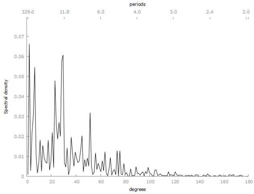
Periodogram of linearly detrended logarithm of aggregate real rye price, 1543–1871. Note: real rye price based on geographically stable sample.
Specification of CF Filter in Robustness Check
To implement the CF filter, we linearly detrend log(Rt) and use the residual, because the filter cannot be applied to trending series (cf. the trend shown in panel (b) Figure 3). To use the CF filter as a high-pass filter, we specify the minimum period as 2 and the maximum period as 20. [118]
About the authors
Hakon Albers is a post-doctoral researcher at Martin Luther University Halle-Wittenberg, where he received his PhD in economics in 2020. He does quantitative research at the intersection of growth & development, economic history, and agricultural economics. He has analyzed agricultural production and trade in different contexts considering the impacts of climate and weather. Recent key publications are: H. Albers/C. Gornott/S. Hüttel, How Do Inputs and Weather Drive Wheat Yield Volatility? The Example of Germany, in: Food Policy 70, 2017, pp. 50-61; and H. Albers/U. Pfister, Climate Change, Weather Shocks, and Price Convergence in Pre-industrial Germany, in: European Review of Economic History 25, 2021, pp. 467-489.
Ulrich Pfister is Senior Professor of Social and Economic History at the University of Münster since 1996. He received his PhD from the University of Zürich in 1984, the Habilitation followed in 1991. His research covers the social and economic history of Europe from the sixteenth to the nineteenth century. He has published in the fields of historical demography, the development of regional export industries, the history of religion, agricultural history and economic growth. Recent publications include: U. Pfister/J.-O. Hesse/M. Spoerer/N. Wolf (eds.), Deutschland 1871. Die Nationalstaatsbildung und der Weg in die moderne Wirtschaft, Tübingen 2021, english version: U. Pfister/N. Wolf (Eds.), An Economic History of the First German Unification. State Formation and Economic Development in a European Perspective, London 2023; and U. Pfister, Economic Growth in Germany, 1500–1850, in: Journal of Economic History 82, 2022, pp. 1071-1107.
Acknowledgement
We are grateful for valuable comments by the editor Jochen Streb, an anonymous reviewer, and seminar participants at the Zurich Virtual Fresh Meeting 2021, the University of Regensburg 2022, and the EHES Conference in Groningen 2022. All errors remain ours.
© 2025 Hakon Albers and Ulrich Pfister, published by De Gruyter
This work is licensed under the Creative Commons Attribution-NonCommercial-NoDerivatives 4.0 International License.
Articles in the same Issue
- Frontmatter
- Nachruf auf Wolfram Fischer
- Special Issue Articles
- Investment and Saving Opportunities for Different Socio-Economic Groups in Medieval and Early Modern Europe
- Politics, Investments and Public Spending in Bologna (End of 13th – First Half of 14th Century)
- Financing Poor Relief in the Small Lower Rhine Town of Kalkar in the Late Middle Ages
- Credit for the Poor, Investments for the Rich? Different Strategies for Investing and Saving Money in Medieval Tirol
- Financing the Commune
- Investing in a New Financial Instrument: The First Buyers of Urban Debt in Catalonia (Mid. 14th Century)
- Set for Life: Old-Age Pensions Provided by Hospitals in Late-Medieval Amsterdam
- Credit Investments in Northern Italian States (17th–18th Centuries)
- Research Forum
- Food Crises in Germany, 1500–1871