Financial Inclusion, Financial Depth, and Macroeconomic Fluctuations
-
Saira Tufail
 and
Mehboob Ul Hassan
and
Mehboob Ul Hassan


Abstract
The study bridges the gap between growth and business cycle literature by addressing two critical issues related to the connection between financial development (FD) and macroeconomic fluctuations (MF). First, it explores strategies for achieving FD in an emerging economy. Second, it examines the extent to which FD can occur while maintaining system stability. To address the first problem, the research evaluates the impact of two main components of FD, financial inclusion and financial depth, on fluctuation, while the second issue examines the impact of different degrees of financial inclusion and depth on macroeconomic volatility. The analysis is extended to consider the influence of demand and supply-side drivers of FD on MF. By introducing theoretical underpinnings of financial depth and access in a large-scale new Keynesian model, the study indicated that the financial sector with low depth and access intensifies fluctuations caused by all shocks, whether real, nominal, or financial. The study also found that for macroeconomic stability in the face of diverse shocks, a medium to high level of depth with a moderate degree of inclusion is essential. Furthermore, it is encouraged to reach a greater degree of FD using supply-side drivers rather than demand-side variables.
1 Introduction
Financial development (FD) has been identified as an important growth driver since the seminal contributions by McKinnon (1973). Lately, its role in the severity and magnitude of macroeconomic fluctuations (MF) has attracted considerable attention from both policymakers and academics across the world. Theoretically, the factors that allow FD to stimulate economic growth should also smooth economic fluctuations. A well-developed financial system mitigates information asymmetries, reduces agency and verification costs, minimizes financial frictions, and cushions economic stability. Resultantly, economies having robust financial sectors (FSs) are thought to be more resilient to shocks and have a higher ability to manage macroeconomic volatilities.
In general, there are two major approaches to model the relationship between fluctuations and FD. The approach followed by growth literature concentrates on numerous aspects of the FD process, like depth and inclusion. It directly assesses their impact on overall measures of macroeconomic volatility, typically overlooking shocks, cycles, and the intricacies of financial structure. In contrast, business cycle literature gives a central position to the shocks that cause fluctuations as well as the role of the economy’s financial structure in the propagation of these shocks, assuming the given FD process.
Empirical evidence surrounding growth literature is growing but ambiguous. The prevailing view supports a non-linear U-shaped relationship where FD dampens macroeconomic volatility up to a point, beyond which further development exacerbates it (Arcand et al., 2015; Dabla-Norris & Srivisal, 2013). This is despite the fact that a number of studies have reported a negative relationship between FD and macroeconomic volatility (Beck et al., 2012, Cevdet et al., 2000; Easterly et al., 2000). The nexus is reported to have varying strengths for different stages of financial and economic development (Kunieda, 2008) and over the short and long term (Darrat et al., 2005; Tiryaki, 2003). Pinheiro et al. (2017) reported a humped-shaped relationship between FD and MF.
Preliminary evidence from business cycle literature like Aghion et al. (1999) showed that the financial markets of less developed countries are typically less stable and grow more slowly. Beck et al. (2006) showed that real shock aggravates growth volatility in the presence of asymmetric information, while the reverse holds for nominal shock. Within the context of the new Keynesian dynamic stochastic general equilibrium (NK-DSGE) model, the empirical insights are more complex. The interplay between a variety of shocks and financial frictions generates a multitude of implications for MF. Nonetheless, existing analyses specify scarce evidence on the decomposition of FD into its characteristics, thus complicating how each characteristic exclusively interrelates with the cyclical properties of variables and leaving much of the richness in fluctuations–FD relationship unexplored.
This clear and significant gap in the literature necessitates additional research efforts in this area as it is of considerable importance for emerging and developing countries that are striving to identify the appropriate level of FD and strategies to achieve that level. Against this background, this study examines the macroeconomic implications of FD, delivering empirical evidence on the relationship between the depth and inclusion of FS and the macroeconomic dynamics generated via nominal, real, and financial shocks. Within the framework of business cycle literature, instead of considering FD as exogenous, we focus on those policy measures that determine the depth and inclusion of FS in the model.
Both financial depth and inclusion are reflective of the success of the FD process. Financial inclusion has multiple definitions and is a multifaceted concept. The most prominent literature in this regard defines it as the availability and utilization of formal financial services (Čihák et al., 2016; Sahay et al., 2015). Financial inclusion has become a formal monetary policy goal for many nations in recent years (Sahay et al., 2015). However, its bearings for macroeconomy are quite an unexplored area of research. Macroeconomic stability and increased resilience of the financial system following the expansion of financial inclusion are expected (Hannig & Jansen, 2011). Contrary to it, financial inclusion, if unregulated, may lead to systemic financial risks due to moral hazard problems (Morgan & Pontines, 2018; Siddiki & Bala-Keffi, 2024).
Like financial inclusion, financial depth is also a double-edged sword. Financial depth is known as the ability of the financial system to provide capital to both the public and private sectors and also ensures the availability of financial services (Bhattacharya & Patnaik, 2016). By determining the size of FS of a particular country relative to its economic size, financial depth eases the liquidity constraints on businesses and promotes long-term investment, which can lower the volatility of growth and investment (Aghion et al., 2010). Nevertheless, there is also the argument that the pro-cyclical nature of FS is increased by the excessive expansion of the sector in relation to the size of the economy in a number of ways, hence amplifying shocks and volatility (Quadrini, 2011).
It is crucial to simultaneously assess the impact of both drivers of FD on economic stability for numerous reasons. First, the sustainability of the FD process may be compromised if one dimension is pursued, while the other is restricted. Second, both factors typically exhibit a bell-shaped relationship with growth and stability, underscoring the need for a simultaneous examination to prevent underestimating the relationship between FD and fluctuations. Additionally, the literature suggests that while financial depth is often assumed to have a bell-shaped relationship with growth and stability, financial inclusion may have a more straightforward, monotonic relationship with growth (Dabla-Noris, 2015; Sahay et al., 2015). This reinforces the necessity for a concurrent examination to determine the optimal levels of both, minimizing the trade-off between FD and cyclical fluctuations.
Given this background, the objectives and major contributions of the study are as follows. First, the existing literature assesses the causal link between the outcomes of the FD process through aggregate measures of depth and inclusion on macroeconomic volatility, which is also measured at the aggregate level. Instead of following an “outcome to outcome”-based approach, we add to the literature by incorporating demand- and supply-side measures of financial depth. Demand-side measures restrict the amount of loans that non-financial borrowers, such as households and businesses, can obtain from financial institutions by operating through their balance sheets. These measures are loan-to-income (LTI) and loan-to-value (LTV) ratios for households and firms, respectively. Supply-side measures operate through the balance sheet of financial intermediaries (like banks) and limit the amount of loans banks can advance. Both demand- and supply-side financial measures determine the amount of credit provisions to the economy and indicate the depth of the FS (Baskaya et al., 2016; Gómez et al., 2019). The percentage of households that are financially included serves as a direct indicator of financial inclusion. In this regard, we hypothesize that policy insights from an “outcome to outcome” are limited only to suggest that either the FD process is leading to or inhibiting MF. However, our study is expected to provide policy prescriptions on how the FD process should proceed without causing macroeconomic instability.
Second, along with exploring the suitable combination of financial depth and inclusion for FD, the study contributes to the literature on a variety of other fronts. For instance, it further investigates the way of increasing financial depth in the economy to reduce MF. Particularly, it sorts out whether financial depth should take place through demand-side measures or supply-side measures. Furthermore, it directly compares the implications of the two most important facets of FD considered in this study.
Although a great deal of research has been done on the effects of FD on growth (Wen et al., 2021), there is a relatively limited body of research that investigates the connection between various aspects of the FD process and economic fluctuations. Similarly, identifying the significance of demand-side and supply-side financial triggers for economic fluctuations remains an underexplored area of study. Additionally, according to Sahay et al. (2015), there is a lack of comprehensive understanding regarding the instability implications of financial inclusion. For instance, in contemporary analysis, Ozili (2020) examined the behavior of financial inclusion over the business cycle; however, the research on how much business cycle fluctuations can be attributed to financial inclusion is in fact scant. This gap in knowledge is even more pronounced in general equilibrium models.
As the effects of FD are faced by all sectors of the economy, it is imperative to explore its significance for the business cycle in a general equilibrium model. In this regard, we estimate the NK-DSGE model for Pakistan using quarterly data from 1972Q1 to 2017QIV to attain the objectives of the study. The research for Pakistan regarding this issue is at an embryonic stage. Majeed and Noreen (2018) is a pioneering contribution. They examined the impact of financial depth, access, stability, and efficiency on output volatility using the “outcome-to-outcome” approach. This study is anticipated to make a significant contribution to the literature by investigating how various policy measures influencing FD affect MF in the face of various nominal, real, and financial shocks. In this regard, the study can be considered the need of time as the government is thriving to improve the worsening credit profile of the country, on the one hand, and intends to pursue the rigorous financial inclusion strategy on the other. The findings of the study can also be suggestive of other developing and emerging countries.
The rest of the study is examined as follows. Section 2 presents the literature review. In Section 3, the data and methodology are presented. Results and discussion are covered in Section 4, and the conclusion is provided in Section 5.
2 Literature Review
2.1 Financial Inclusion and Macroeconomic Fluctuations
Only a handful of studies can be found on the role of financial inclusion for MF in growth literature. First, financial inclusion is reported to have a strong smoothing effect on MF with the efficient intermediation of financial resources between savers and investors, a wider range of economic agents, diversification of financial activities, and, hence, higher financial resilience (Khan, 2011). According to Morgan and Pontines (2018), financial inclusion is a useful strategy for lowering the likelihood of bankruptcy. They showed by extending financial services to small and medium enterprises, banks can effectively reduce non-performing loans; hence, the overall risk banks can encounter. Evidence on reducing output volatility through consumption smoothing as a result of greater access to financial services also provides a strong case for financial inclusion. The findings of Mehrotra and Yetman (2014) indicate that increased household access to financial services for borrowing and saving activities reduces output volatility. It also hinders the growth of the substantial informal sector (García & José, 2016).
On the other hand, Sahay et al. (2015) depicted that the benefits of financial inclusion fade with more inclusion, and it may become a cause for increased instability in the FS. García and José (2016) argued that financial inclusion may increase risks in financial markets, thus leading to macroeconomic instability. Similarly, according to Morgan and Pontines (2018), financial inclusion increases economic and financial instability by opening up financial services to borrowers who pose a risk by loosening lending requirements. As a result, it might lower credit quality and cause credit to grow at an unprecedented rate (Mehrotra & Yetman, 2014). Nonetheless, increases in financial instability and credit risk associated with higher financial inclusion occur only in fragile economies (Siddiki & Bala-Keffi, 2024). According to López and Winkler (2019), it remains a policy challenge to expand financial inclusion without contributing to a potentially destabilizing credit boom.
Apart from these two distinct effects, empirical evidence also revealed a U-shaped relationship between financial inclusion and macroeconomic stability. According to Vo et al. (2019), financial inclusion was found to improve financial stability up to a certain point, after which the relationship was found to be reversed. It was also discovered that financial inclusion helped to limit inflation and stabilize output growth.
In business cycle literature, the concept of financial access is incorporated implicitly in macroeconomic models by incorporating financially excluded or rule-of-thumb households. The research related to the implication of financial inclusion for business cycle fluctuations in the DSGE framework particularly and in overall macroeconomic literature, generally, is limited. Although a few studies have taken financially excluded households into their modeling approach (Coenen & Straub 2004; De Graeve, 2008; Gali et al., 2004; Galí et al., 2007; Mankiw, 2000), neither have they considered it as a characteristic of FD process, nor have examined its implication for macroeconomic stability.
2.2 Financial Depth and MF
Early findings in the literature on growth indicated that lending to the private sector plays a significant role in reducing variations in output and consumption (Easterly et al., 2000). Additionally, Cevdet et al. (2002) argued that less variation exists in output, consumption, and investment growth in nations with highly developed FSs, indicating that the percentage of private credit accounts for the majority of volatility. Tiryaki (2003), instead, demonstrated that the link between FD and business cycle volatility is not straightforward in the short run. The findings of the study showed that though investment volatility reduced following the development of FS, output fluctuations largely remained irresponsive to FD owing to the positive link between consumption volatility and FD. Darat et al. (2000) supported the theoretical contention that financial depth has a strong mitigating effect on growth volatility in the long run; however, in the short run, the effects are insignificant.
Similarly, many studies reported a non-linear U-shaped relationship between FD and MF. A significant contribution is Dabla-Norris and Srivisal (2013). They demonstrated that financial depth considerably reduces the volatility of output, consumption, and investment growth but only to a limited extent. Financial depth increases investment and consumption volatility at very high levels, as seen in many advanced economies. They also showed that the negative effects of external shocks on macroeconomic volatility are lessened by deeper financial systems acting as shock absorbers. Ma and Song (2018) found a substantial U-shaped impact of financial depth on macroeconomic volatility which is more pronounced with a larger FS.
Although the literature on business cycles does not specifically model the degree of FD as a cause of instability, it is implied that financial institutions and intermediaries can reduce overall volatility if they are able to reduce or even eliminate friction. Theoretically, a developed financial system encourages risk sharing and loosens lending restrictions, which strengthens the economy’s resilience to shocks. In particular, in economies with stringent international financial constraints, deeper financial systems can reduce the cash constraints of firms and hence reduce volatility. Aghion et al. (1999) supported the theoretical conjectures and showed that economies with less developed financial systems tend to be more volatile as investors are locked out of credit markets due to imperfections in the advent of an adverse shock. Nonetheless, Pinheiro et al. (2017) showed that reducing financial frictions may generate opposite effects in the forms of reallocation of productive inputs and change in demand for inputs. The theoretical model developed by Beck et al. (2006) predicted that financial intermediaries have a magnifying effect on the spread of monetary shocks and a dampening effect on the spread of real shocks. Their empirical data demonstrated that the overall impact of financial depth on growth volatility is negligible because of the financial intermediaries’ contradictory roles for both real and monetary shocks. Aghion et al. (2010) showed that the cyclical properties of long-term investment change substantially in complete markets as compared to financial markets with tight constraints.
Several noteworthy observations arise from the literature review above, emphasizing the significance of the present study in contemporary literature. Modeling of demand- and supply-side metrics of financial depth, along with the integration of financial inclusion into the business cycle literature, represents an unexplored research area for emerging and developing economies. Additionally, the existing literature for these economies lacks insight into the dynamic interaction among various aspects of the FD process and their implications for the macroeconomy. This study is anticipated to offer pioneering evidence, advocating for the inclusion of FD policies in DSGE literature.
3 Methodology and Data
The DSGE model, as used by Gerali et al. (2010) and Hollander and Liu (2016), is utilized to examine the influence of financial depth and inclusion on MF. Gerali et al. (2010) focused on the housing sector, while Hollander and Liu (2016) considered the equity price channel. We have included financially excluded households in the model and did not consider housing and equity prices in our model. Our main contribution is to analyze state-of-the-art models for different drivers of FD. Utilizing contemporary macroeconomic theory, the DSGE models conduct policy analysis and provide an explanation and forecast for the co-movements of aggregate time series throughout the business cycle. The DSGE models are used primarily for forecasting, transmission mechanisms, and policy experiments. The use of the DSGE model is compatible with the objectives of the research as we intend to examine the transmission of different aspects of FD to economic fluctuations through different simulation experiments. The optimal combination of financial depth and access is ascertained through forecasting. The DSGE models are solved through either calibrations or estimations. The model in this study is estimated with quarterly data. For some of the parameters in the estimations, the prior distribution must be specified; for the remaining parameters, fixed priorities are provided. This is done in Section 3.3.
Households, businesses, and the FS make up the model economy. Numerous nominal and real rigidities are incorporated into the model, including incomplete indexation, staggered price and wage rigidities in the Calvo style, variable capital utilization, accumulation of habit stock by households, and investment adjustment costs. The model hosts two real, one monetary, and four financial shocks. The model is equipped with cutting-edge features and is provided in detail in the reference mentioned. The main equations of the model are presented in the Appendix, and their log-linearized form is presented here.
3.1 Theoretical Model
The model is organized with respect to each sector considered in this study.
3.1.1 Household Sector
There are two types of households. First, there are households that maximize their lifetime utility under an intertemporal budget constraint, known as Ricardian or intertemporally optimizing households. Due to their access to capital markets, these households are able to save or borrow money. The latter group, known as rule-of-thumb or non-Ricardian households or financially excluded, uses up all of their current labor income and is unable to access capital markets. Presumably,
Within Ricardian group R = {S, B}, both representative households maximize expected lifetime utility considering a CRRA utility function with distinct consumption preferences
The savers’ households allocate income from the labor market (
A combination of intra-temporal trade-offs between working hours and consumption, as well as intertemporal substitution in consumption, results in aggregate consumption that revolves around real interest rates
For borrowers’ households, the Euler equation takes the following form:
The log linearized form of borrowers’ borrowing constraint is given as follows:
where
Following Gerali et al. (2010),
where
The consumption of financially excluded households is given as follows:
For intermediate good producers, households provide differentiated labor and while, wages are set in a staggered pattern with a constant Calvo probability
The remaining households’ wages are partially indexed using
In addition to wage mark-up and a cost-push shock to wages
3.1.2 The Production Sector
The production sector is made up of perfectly competitive final goods producers who combine the intermediate goods to create homogenous final goods and monopolistically competitive firms that produce intermediate goods. Aggregate output
where
Furthermore, the optimal capital utilization rate is obtained by equating the cost of increased capital utilization with the capital service rental price
The marginal product of capital is denoted as
The following is the marginal product of labor that also arises from the firm’s cost minimization problem:
Monopolistically competitive firms likewise follow staggered contracts in price settings similar to wages. Following Calvo setting, a number of firms are able to revise their prices using constant Calvo probability
Equation (13) represents a hybrid NK price Philips curve, where the backward-looking portion results from partial indexation, and the forward-looking behavior is represented by the expected future inflation term
3.1.3 Investment and Entrepreneurs
In order to derive the Euler equation for investment, one must assume that new capital stock
Comparable to consumption, the value of installed capital
Given the log-linearized standard capital accumulation equation
The current value of installed capital
where
Entrepreneurs maximize utility from consumption and finance by renting capital to intermediate goods producers and borrowing from banks. The key factor depicting the level of FD arises with the assumption that entrepreneurs need collateral to take loans. The following is the Euler equation for entrepreneurial consumption:
Entrepreneurial loans are subject to the following collateral constraints:
where the maximum permissible leverage ratio is determined by the LTV ratio, represented by
3.1.4 Banking Sector
The structure of the banking industry complies with Gerali et al. (2010). The banking industry is made up of a range of commercial banks that compete monopolistically. Two monopolistically competitive retail branches – the loan and deposit branches – and one perfectly competitive wholesale branch, make up each Bank (j). The deposit branch collects deposits from households and deposits them at the wholesale branch. Because the wholesale deposit rate
The bank capital evolves as follows:
The retail loan branch collects loans from the wholesale branch and advances them to borrowers’ households and entrepreneurs at differentiated rates,
where z = {borrower households, entrepreneurs}. The equation illustrates how the loan rate setting is influenced by the stochastic mark-up, past and expected loan rates, the wholesale loan rate, and the marginal cost of the loan branch determined by the policy rate and the bank’s balance sheet position.
3.1.5 Aggregation
Because of the resource constraint, the aggregate output is divided into four categories: government spending, investment goods, consumption, and resources lost due to variable capital utilization
where the steady-state percentages of GDP for household consumption, investment, and capital utilization loss are
3.2 Financial Depth and Access in Model
Financial access is measured by the proportion of financially included households, that is,
Both LTI and LTV show the demand-side determinants of financial depth, while
The respective values are
The model is estimated using the Bayesian estimation technique. Bayesian methods allow researchers to assess and estimate a broad spectrum of macro models that are often challenging for traditional econometrics. The use of Markov chain Monte Carlo (MCMC) simulators to estimate and assess medium- to large-scale DSGE models has made more computational power available, which has added to the appeal of the Bayesian approach.
3.3 Data and Transformation
We estimated the model for Pakistan using the Bayesian method with five observables. This section comprises information about data and its transformation, calibrated parameter values, and the prior and posterior distributions of estimated structural parameters.
The data encompasses five observables: output, inflation, interest rate, investment, and consumption, and it spans the years 1972QI to 2019QIV. International Finance Statistics has been used as a data source for variables. Due to the log-linearized nature of the model, the percentage deviation of each variable from the deterministic steady state is taken. Data are converted in accordance with Pfeifer (2014) to ensure that the observables are consistent with the variables in the model. To be more precise, all of the variables are first converted into log form and deseasonalized. Since output and investment are trending variables, a one-sided HP filter is used to detrend them. The outcome variables have a mean of 0 and show the long-term trend deviation. Both interest rates and inflation have a direct stationary equivalent in data since they are stationary variables. The percentage deviation of gross inflation and gross interest rate from a corresponding time-varying steady state or trend has been taken in order to match these variables with log-linearized variables in the model. The quarterly gross interest rate was obtained from the fourth-order geometric mean of the annualized net interest rate. Representatively,
3.4 Priors Distribution
The Bayesian estimation technique is used to estimate some of the model’s parameters using the observed variables mentioned above. Columns 3–5 of Table 1 report the structural parameter priors, and columns 6–9 display the estimated posterior statistics. In a similar way, Table 2 presents the prior and posterior distribution of the shock parameters and persistence coefficient. The prior distribution is standard because we derived our study’s priors from the DSGE literature. For information on the prior distribution of the majority of the parameters taken into consideration for estimation, we consult Gilchrist et al. (2009), Kamber et al. (2015), and Smets and Wouters (2003).
Prior and posterior distribution of structural parameters
| Parameters | Description | Prior distribution | Posterior distribution | ||||||
|---|---|---|---|---|---|---|---|---|---|
| Dist. | Mean | St. dev | Mode | St. dev | Mean | 10% | 90% | ||
|
|
Habit persistence | Beta | 0.70 | 0.10 | 0.78 | 0.05 | 0.80 | 0.78 | 0.80 |
|
|
Intertemporal elasticity of substitution | Normal | 1.5 | 0.375 | 2.2 | 0.25 | 1.69 | 1.16 | 2.22 |
|
|
Frisch elasticity of labor supply | Normal | 2.0 | 0.75 | 1.79 | 0.76 | 1.98 | 0.76 | 3.11 |
|
|
Degree of wage stickiness | Beta | 0.5 | 0.10 | 0.90 | 0.13 | 0.44 | 0.37 | 0.52 |
|
|
Degree of price stickiness | Beta | 0.5 | 0.10 | 0.77 | 0.15 | 0.73 | 0.69 | 0.77 |
|
|
Investment adjustment cost | Normal | 4 | 1.5 | 1.83 | 1.38 | 2.2 | 0.23 | 3.92 |
|
|
Interest rate smoothing | Beta | 0.70 | 0.10 | 0.84 | 0.02 | 0.97 | 0.96 | 0.98 |
|
|
Response to inflation | Gamma | 1.5 | 0.25 | 1.12 | 0.21 | 0.87 | 0.76 | 0.97 |
|
|
Response to output | Gamma | 0.5 | 0.10 | 0.001 | 0.13 | 0.43 | 0.29 | 0.57 |
|
|
Leverage adjustment cost | Gamma | 4 | 2 | 7.14 | 2.4 | 7.4 | 6.95 | 7.84 |
|
|
Entrepreneur interest adjustment cost | Gamma | 4 | 2 | 1.89 | 0.69 | 2.2 | 2.07 | 2.32 |
|
|
Household interest adjustment cost | Gamma | 4 | 2 | 0.81 | 0.56 | 0.85 | 0.75 | 0.95 |
Prior and posterior distribution of shock processes
| Parameters | Description | Prior distribution | Posterior distribution | ||||||
|---|---|---|---|---|---|---|---|---|---|
| Dist. | Mean | Parameters | Mode | St. dev | Mean | 10% | 90% | ||
|
|
Shock to LTI ratio | Beta | 0.6 | 0.2 | 0.75 | 0.22 | 0.62 | 0.31 | 0.91 |
|
|
Shock to LTV ratio | Beta | 0.6 | 0.2 | 0.65 | 0.05 | 0.78 | 0.7 | 0.86 |
|
|
Shock to interest elasticity to households | Beta | 0.6 | 0.2 | 0.94 | 0.05 | 0.92 | 0.9 | 0.96 |
|
|
Shock to interest elasticity to entrepreneurs | Beta | 0.6 | 0.2 | 0.66 | 0.05 | 0.65 | 0.63 | 0.68 |
|
|
Productivity shock | Beta | 0.6 | 0.2 | 0.66 | 0.004 | 0.97 | 0.96 | 0.98 |
|
|
Wage mark-up shock | Beta | 0.6 | 0.2 | 0.6 | 0.28 | 0.57 | 0.28 | 0.98 |
|
|
Price mark-up shock | Beta | 0.6 | 0.2 | 0.05 | 0.001 | 0.973 | 0.972 | 0.976 |
|
|
Interest rate shock | Beta | 0.6 | 0.2 | 0.90 | 0.06 | 0.12 | 0.03 | 0.23 |
|
|
Shock to LTI ratio | Inv. Gamma | 0.10 | 2 | 0.86 | 0.12 | 0.62 | 0.31 | 0.91 |
|
|
Shock to LTV ratio | Inv. Gamma | 0.10 | 2 | 0.05 | 0.018 | 0.01 | 0.008 | 0.012 |
|
|
Shock to interest elasticity to households | Inv. Gamma | 0.10 | 2 | 0.06 | 0.014 | 0.02 | 0.016 | 0.03 |
|
|
Shock to interest elasticity to entrepreneurs | Inv. Gamma | 0.10 | 2 | 0.04 | 0.018 | 0.04 | 0.02 | 0.06 |
|
|
Productivity shock | Inv. Gamma | 0.10 | 2 | 0.05 | 0.014 | 0.03 | 0.02 | 0.04 |
|
|
Wage mark-up shock | Inv. Gamma | 0.10 | 2 | 0.04 | 0.01 | 0.07 | 0.02 | 0.11 |
|
|
Price mark-up shock | Inv. Gamma | 0.10 | 2 | 0.01 | 0.001 | 0.01 | 0.008 | 0.011 |
|
|
Interest rate shock | Inv. Gamma | 0.10 | 2 | 0.007 | 0.0003 | 0.007 | 0.006 | 0.008 |
Note: The prior distribution is obtained from three chains of Metropolis Hasting algorithm.
The following distributions are assumed to correspond to the parameters governing the utility function. According to a beta distribution, the mean value of habit persistence is set at 0.7 with a standard error of 0.1. In DSGE models, the value is thought to be consistent in avoiding consumption and equity premium puzzles. Both the labor supply elasticity and the intertemporal elasticity of substitution are set at 2 with a standard error of 0.75 and 1.5, respectively, with a standard error of 0.375. These values are expected to follow a normal distribution.
It is assumed that the parameters that determine the setting of wages and inflation follow the beta distribution. Prices and wages have probabilities of approximately 0.5 for Calvo staggered contracts, meaning that these contracts have an average duration of 6 months. In the labor and goods markets, the prior mean of the degree of indexation to previous inflation is likewise fixed at 0.5.
The Taylor rule’s parameters are as follows: a gamma distribution with a mean of 1.5 and 0.50 and standard errors of 0.25 and 0.10, respectively, characterizes the long-run feedback on output growth and inflation. It is assumed that the lag in interest rates, which indicates the persistence of the policy rule, is beta-distributed with a standard error of 0.1 and a mean of 0.70.
As far as possible, the prior distributions for stochastic processes and persistence are consistent. For every innovation, an inverse gamma distribution with a mean of 0.10 and two degrees of freedom is assumed. It is assumed that the persistence of all AR(1) processes has a beta distribution with a mean of 0.6 and a standard deviation of 0.2.
3.5 Calibrated Parameters
Since there is insufficient information in the data on some observables to account for all the parameters, the remaining parameters are treated as fixed priors. In order to calibrate parameters for the Pakistani economy, we consulted multiple sources. As a reciprocal of the steady-state quarterly gross interest rate,
Parameters’ calibration
| Parameter | Description | Value | Estimation | Data/reference |
|---|---|---|---|---|
|
|
Discount factor for savers’ households | 0.998 | Data | Quarterly data/IMF |
|
|
Discount factor for borrowers’ households | 0.96 | Literature | |
|
|
Discount factor for entrepreneurs | 0.95 | Literature | |
|
|
Discount factor for bank | 0.998 | Literature | |
|
|
Depreciation rate | 0.025 | Data | Annual data/SBP and Penn World Table. Parameters adjusted for quarterly response |
|
|
Depreciation rate for banks | 0.1 | Literature | |
|
|
Curvature of Dixit-Stigler aggregator | 6 | Literature | Choudhri and Malik (2012) |
|
|
Share of capital in production | 0.49 | Cointegration | Annual data/coefficients adjust for quarterly response |
|
|
Elasticity of capital utilization | 0.54 | Literature | |
|
|
Proportion of sticky prices | 0.08 | Literature | Ahmed et al. (2012) |
|
|
Curvature of Dixit-Stigler aggregator | 6 | Literature | Choudhri and Malik (2012) |
|
|
Entrepreneurial survival rate | 0.99 | Literature | Bernanke et al. (1999) |
| Steady-state values in model economy | ||||
|
|
Consumption to GDP ratio | 0.80 | Data | Handbook of Statistics on Pakistan Economy |
|
|
Entrepreneurial consumption to GDP ratio | 0.01 | Literature | |
|
|
Investment to GDP ratio | 0.18 | Data | Handbook of Statistics on Pakistan Economy |
|
|
Proportion of output lost due to capacity utilization | 0.01 | Literature | |
|
|
Steady-state level of capital to net worth ratio | 1.24 | Data | Firms’ annual financial accounts by SBP |
Source: Authors’ tabulation.
3.6 Posterior Distribution
Table 1 shows the posterior distribution of the structural parameters. It was found that the posterior estimate for habit formation was statistically significant at 0.78. According to Havranek et al. (2017), the US, EU, OECD, and Japan had mean values of habit formation that were closer to 0.73 out of 129 estimated DSGE models. Numerous studies, however, have indicated that this estimate falls between 0.8 and 0.9. A higher value of habit stock is more likely for EDEs positioned closer to the left tail of the income distribution.
Our results conform to widespread literature on price and wage stickiness, which reported comparatively more frequent price changes than wage changes. The result showed that the average wage contract withstands longer than the average price contract. The estimated value of the adjustment cost parameter 2.2 is significantly higher than the value found in previous research involving financial frictions. Because capital adjustment costs are higher, capital prices are more susceptible to shocks and increase the volatility of net worth. The price of external funding is directly impacted by higher adjustment cost. Higher adjustment cost also implies that the investment is more costly and less shock-tolerant.
A much higher level of interest rate smoothing is revealed by the monetary policy rule’s lagged policy coefficient (0.86). The rigidity of prices can be partially explained by the central bank’s slow adjustment process. The output gap and inflation response coefficients are 0.03 and 1.20, respectively. Regarding the estimates of reaction coefficients in monetary policy rules, there is no consensus in Pakistan. For example, Malik and Ahmed (2010) argued that Pakistan’s monetary policy is highly accommodating since the weights assigned to output (0.19) and inflation (0.32) in the monetary policy rule deviate significantly from Taylor’s recommendations. However, Haider and Ramzi (2009) demonstrated that the estimated coefficients (1.17 and 0.72), when considered in the context of the DSGE model, are more in line with the Taylor rule’s conjecture. The estimated coefficients of this study are closer to Haider and Ramzi (2009) for inflations where monetary policy pursues inflation targeting steadfastly pursuing growth as a secondary objective.
The estimated shock persistent coefficients show that monetary policy shock is most persistent followed by productivity shock and financial shock to households and entrepreneurs. Given their high persistence, these shocks are likely to be responsible for the majority of the endogenous variable forecast error variance over the long term. In that instance, as indicated by the low value of their standard deviations, both the financial and interest rate shocks were less enduring and less volatile.
3.7 Stylized Facts
Figure 1 compares the financial Development Index of Pakistan with low-income and developing countries, Asia and Pacific, and Emerging economies, while Figure 2 displays different constituents of the FD process. Both figures highlight regional disparities in the pace of FD, with Pakistan showing inconsistent performance. Figure 3 contains the overview of major macroeconomic variables (measured in growth rate form) and their volatilities (3 years moving standard deviation). Figure 3 shows that GFCF and GDP growth exhibit periods of negative or low growth, reflecting economic downturns while consumption appears relatively stable. Similarly, volatility in GFCF and GDP growth seems to be higher than in other variables, especially post-2000, suggesting greater investment and growth uncertainties.

FD. Data source: International Finance Statistics (2024).

Financial depth and access. Data source: International Finance Statistics (2024).

Major macroeconomic conditions of Pakistan. Data source: International Finance Statistics (2024).
Figure 4 contains information on the two-way relationship between the volatilities of major macroeconomic variables and different indicators of FD. Overall, FD and all of its components generally increase inflation volatility. On the contrary, output volatility reduces or remains unresponsive to FD and its constituent except for the financial institution access index. Investment becomes more volatile with an increase in financial market access, which significantly reduces consumption volatility.

FD and volatility of major macroeconomic variables.
4 Results and Discussion
This section presents the results pertaining to the objectives of the study.
4.1 Financial Depth, Inclusion, and Severity of Business Cycle Fluctuations
In this section, results pertaining to the study’s first research question are presented. The effect of varying degrees of financial depth is examined by setting the model for full inclusion. Similarly, to assess how financial inclusion has affected, a medium level of financial depth is considered. Low inclusion case corresponds to the situation where 50 percent of households are financially excluded, high inclusion with 20 percent, and full inclusion where all households interact with financial markets. Comparing models with different degrees of financial depth with fixed inclusion and with different extents of financial inclusion with fixed levels of financial depth, we examine the impact of depth and inclusion on the severity of the business cycle using impulse response functions.
4.1.1 Cost-Push Shock
Figure 5 shows the response of key macroeconomic aggregates on an adverse cost-push shock (depicted in equation (12)) for low, medium, and high levels of FD without considering financial exclusion. Cost-push shock is contractionary for output. Although aggregate consumption, working hours, and loans advanced also reduce; nonetheless, at disaggregated levels, dynamics vary across savers and borrowers and households and entrepreneurs. Savers’ households pay the cost of shock in terms of foregone consumption, whereas both entrepreneurs’ and borrowers’ households are better off in terms of consumption. This may be attributed to the decrease in interest rates for both households and entrepreneurs on their loans. A decrease in interest rate induces entrepreneurs’ loans to increase leading to a higher level of investment. Moreover, the passing-on of an increase in cost to prices is also indicated in a higher level of inflation in response to shock. This induces the policy rate to increase in impact, and its effectiveness in controlling inflation is ubiquitous in the longer term.

Cost-push shock for varying degrees of financial depth (left) and access (right).
It is evident from the figure that the effect of cost-push shock on macroeconomic aggregate is efficiently mitigated in the environment with higher and medium levels of financial depth. A low level of financial depth enhances the cyclicality of macroeconomic aggregates substantially. This implies that a well-developed financial system insures entrepreneurs against cost-push shock and results in the level of economic contractions far below than in a system with inadequate financial depth. This conforms to the findings of Beck et al. (2002), who deliberate that the development of financial intermediaries enhances the macroeconomic volatility in the face of real shock.
Figure 5 also presents the MF arising in response to an adverse cost-push shock in an economy with three levels of financial inclusion and a medium level of financial depth. In a model for different levels of financial inclusion, a positive cost-push shock generates an impact contraction for the output and consumption for 9 quarters, while employment contractions persist for 17 quarters. The response to inflation and interest rate is positive, while in the long run, a decline is observed before returning to the equilibrium level. Financial inclusion of different extents attenuates the negative impact of shock for output, employment, and wages, while for inflation and interest rate, negligible impact differences are found in responses. Low financial inclusion makes the shock persist for longer.
The shock propagates similarly to the above case, where full inclusion is considered with different levels of financial depth. However, contrary to the above case, where a lack of financial depth magnifies the adversity of shock, higher financial inclusion magnifies fluctuations in output and aggregate working hours, while for the rest of variables, high exclusion is observed to magnify the impact of shock, particularly for loans advanced. The findings reveal that FD, through the increase in financial inclusion, mitigates the contraction arising from cost-push shock. Moreover, the general overview of results indicates high inclusion as a favorable policy option for FD instead of full inclusion.
4.1.2 Productivity Shock
The production function presented in equation (7) specifies the productivity shock. Macroeconomic expansion follows in response to a positive productivity shock, as presented in Figure 6. Overall, the responses of key macroeconomic variables are consistent with previous research. The easing of policy interest rate and its effectiveness in reducing inflation in the face of productivity shock is ubiquitous in the current model. Neither the magnitude nor the persistence of productivity shock is responsive to the level of financial depth except for policy rate and savers’ consumption. Our results for consumption conform to Bhattacharya and Patnaik (2016) report that consumption is more volatile when financial inclusion increases.

Productivity shock for varying degrees of financial depth (left) and access (right).
The bearing of productivity shock for business cycle fluctuations is not independent of the different levels of financial inclusion. Output and aggregate consumption increase remarkably higher for full inclusion cases as compared to cases where the financial market is segmented. For monetary and financial variables, low inclusion is magnifying and causing the effect of shock to persist. It is also observed that the positive impact of favorable productivity shock on output and consumption is highest in the full inclusion case, but the impact persists longer for the high inclusion case. This indicates that though productivity shock propagates to key aggregates similarly for all three cases of financial inclusion, nonetheless, amplification and persistence of shock vary to different extents.
4.1.3 Monetary Policy
The responses of the main macroeconomic variables to the unanticipated monetary policy shock shown in the Taylor rule are plotted in Figure 7. Real economic variables decline in response to a contractionary monetary policy shock, with a peak response occurring in the fourth quarter. The strength of the monetary transmission mechanism and the average lag time of the economy’s reaction to monetary policy actions are both supported by the conventional evidence in these responses. Amplification and persistence of monetary shock are evident for low levels of FD.

Monetary policy for varying degrees of financial depth (left) and access (right).
On impact, the response of macroeconomic variables to monetary contraction is not substantially different for the three levels of financial inclusion. The amplification and persistence of monetary contraction over an extended horizon varies moderately with the change in financial inclusion. Particularly for real variables persistence is high for high inclusion. Interest rate inertia, which is observed for all three cases, is substantial for low inclusion cases. Consequently, more contractions are faced by the economy characterized by highly financially inactive households in the face of monetary policy shock.
4.1.4 LTI and LTV Shock
The favorable shock to LTI ratio on households’ borrowings, as specified in equations (3) and (4), induces households to borrow more and increase their consumption. Loans to entrepreneurs are crowded out and cannot get momentum even with remarkable monetary easing. Consequently, investment happens to be counter-cyclical in the face of LTI shock. However, due to an increase in aggregate consumption, output increases. Working hours are also pro-cyclical. The results show that the easing of macro-prudential regulations induces consumption-led growth in the economy.
The on-impact response of different variables is sensitive to the degree of financial depth. The low level of financial depth enhances the magnitude of pro-cyclical responses and reduces the severity of counter-cyclicality in variables. However, its impact on the persistence of shock is not remarkable. This is not the case for models analyzing the impact of different levels of financial inclusion. The impact of easing the LTV on key macroeconomic aggregate is sensitive to the extent of financial inclusion. An expansionary macro-prudential shock induces output to increase marginally, only in case of full financial inclusion. The cyclical behavior of variables induced by macro-prudential shock is largely dampened in the low-inclusion cases (Figure 8).

LTI shock for varying degrees of financial depth (left) and access (right).
Due to the favorable shock to LTV ratio (mentioned in equation (18)), entrepreneurs’ borrowings increase and converge to equilibrium after the fourth quarters. Investment, working hours, and loans are pro-cyclical, while aggregate consumption is counter-cyclical. The FD occurring through an increase in financial depth only affects the on-impact response of the variable shock which is generally high in case of low financial depth. Otherwise, a financial system with medium and high levels of financial depth moderates positive financial innovation (Figure 9).

LTV shock for varying degrees of financial depth (left) and access (right). Source: Impulse responses are retrieved from Dynare.
From the general overview of the results, a few findings are worth mentioning. Financial depth is an important factor in mitigating the negative impact of both nominal and real shocks. It also increases the favorability of productivity shocks for the economy. However, favorable shocks originating from FS are better realized in an environment with low financial depth. Similarly, adverse shock originating from FS is better mitigated in a low financial depth environment. Another important finding of the study reveals FS as a shock absorber in the case of both nominal and real shocks, however, a catalyst for financial shocks.
4.2 Financial Depth or Financial Inclusion: What Matters More for Business Cycle Fluctuations?
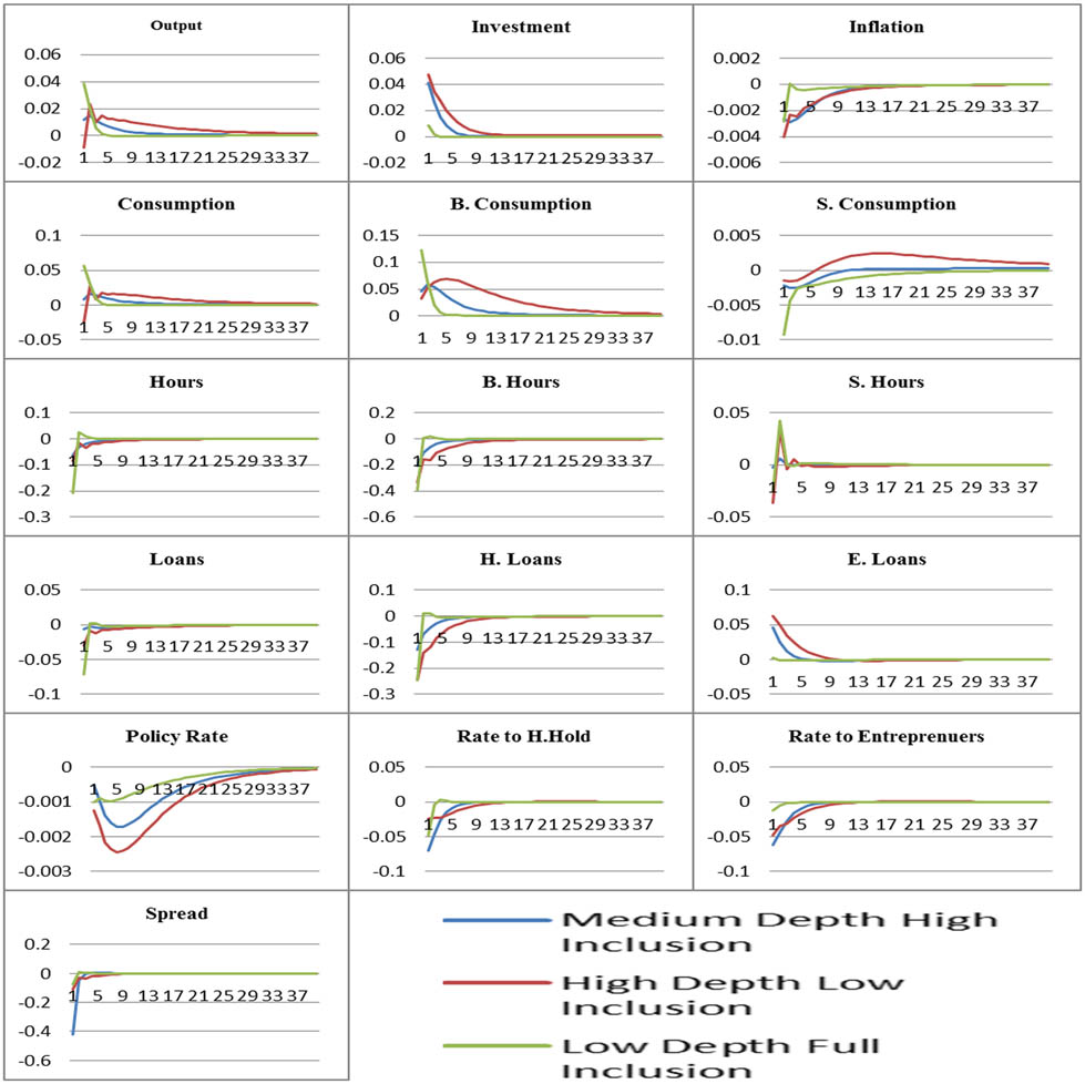
In the above section, we examined the role of financial depth (inclusion) at a particular level of financial inclusion (depth) for business cycle fluctuations in the face of various shocks. The impulses for three combinations are: (a) high depth and low inclusion (HDLI); (b) medium depth and high inclusion (MDHI); and (c) low depth and full inclusion (LDFI) are reported in Figures 10–15.

Cost-push shock. Source: Impulse responses are retrieved from Dynare.
Productivity shock. Source: Impulse responses are retrieved from Dynare.

Monetary policy shock. Source: Impulse responses are retrieved from Dynare.

LTI shock. Source: Impulse responses are retrieved from Dynare.

LTV shock. Source: Impulse responses are retrieved from Dynare.

Household interest elasticity shock. Source: Impulse responses are retrieved from Dynare.
The response of key macroeconomic variables to different shocks shows that the combination of financial depth and inclusion matters for business cycle fluctuations along with the variables and shocks under consideration. For instance, cost-push shock is evidently mitigated in an environment characterized by MDHI or HDLI. While LDFI causes severe contractions in the economy in the face of cost-push shock. Similarly, except for the on-impact responses of output and consumption, the favorable impact of productivity shocks is realized over a longer horizon in the MDHI or HDLI case. The impact of monetary policy shock is highly sensitive to the financial regime assumed. An FS characterized by MDHI neutralizes the adverse impact of contractionary monetary policy shock. The severity of business cycle fluctuations is heightened with the increase in financial depth and decrease in inclusion. For both demand-side positive and supply-side negative financial shocks, the FS with MDHI completely absorbs the impact of shock irrespective of their favorability and adversity, respectively.
4.3 Financial Depth through Demand or Supply Side: What Matters for Business Cycle Fluctuation?
Figures 16–21 compare the role of financial depth achieved either through relaxing demand-side frictions or supply-side friction for the magnitude and longevity of business cycle fluctuations. The results show that the propagation of real shocks to the economy is similar irrespective of how financial depth takes place. For cost-push shock, the magnitude of shock accelerates in the long run when demand-side financial frictions are relaxed. However, for productivity shock, the difference arises in the on-impact response of the shock, which is attenuated in the case when financial depth takes place by relaxing demand-side financial frictions. The persistence of the shock is indifferent to the way financial depth is taking place. The magnitude of the responses of key macroeconomic aggregates for monetary policy shock is slightly different for two cases of financial depth. For most variables, relaxing demand-side financial frictions increase the cyclicality of variables slightly, both in terms of severity and persistence.

Cost-push shock. Source: Impulse responses are retrieved from Dynare.

Productivity shock. Source: Impulse responses are retrieved from Dynare.

Monetary policy shock. Source: Impulse responses are retrieved from Dynare.

LTI shock. Source: Impulse responses are retrieved from Dynare.

LTV shock. Source: Impulse responses are retrieved from Dynare.

Interest elasticity shock. Source: Impulse responses are retrieved from Dynare.
Considerable difference in the transmission, amplification, and persistence of responses is observed for LTV shock which is almost non-existent for LTI shock. In the face of LTV shock, easing demand-side financial frictions gives rise to a substantial contraction in most of the real variables, while easing supply-side frictions generates no added effect on the transmission of shock. Similar findings can be observed when the shock is given to the interest elasticity of loans advanced to households. However, for the shock to interest elasticity faced by entrepreneurs on their loans, financial depth taking place through easing the demand side of supply-side financial frictions is immaterial.
5 Conclusion and Recommendations
In this study, we have examined the importance of different characteristics of the FD process for MF. In particular, we have compared the role of financial depth and financial inclusion for macroeconomic stability. In the context of the new Keynesian DSGE model estimated for Pakistan, the findings of the study showed that financial depth and inclusion have very important implications for MF. First, low depth and low inclusion are magnifying for all shocks, whether real, nominal, or financial shocks. Second, medium depth combined with high inclusion or high depth with low inclusion moderate business cycle fluctuation in the face of most of the shocks. Third, the financial depth taking place by increasing the credit supply dampens the impact of most of the shock. The results of the study clearly indicate that a medium to high level of depth with a moderate level of inclusion is required for macroeconomic stability in the face of various shocks.
The findings of research in this regard have important implications for policies aiming at FD of the country. On the basis of prevailing finance–macroeconomic linkages, the findings of the study suggest concentrating more on financial depth with a medium level of financial inclusion. It implies that with a very high level or full financial inclusion, the system may become more volatile, giving rise to financial instability. It further implies that in its current capacity, the economy’s financial system is not capable of dealing with problems associated with high or full levels of financial inclusion like breaching of debt enforceability contracts and moral hazard problems that arise due to incomplete information. Apart from it, financial exclusion in EDEs is a multidimensional phenomenon, and reducing it to have high inclusion requires major changes in the financial landscape of the economy, which is challenging and requires a long-term strategy. This implication is further supported by the findings of another exercise in this research, which showed that financial depth should be undertaken by relaxing supply-side constraints instead of demand-side constraints, as easy demand-side constraints would also complement the financial inclusion process.
Research regarding the link between FD and MF may be extended in an important way. Hence, the first limitation of the study, that is, the models used in various exercises of this study are all closed economy models. Future research assessing the macroeconomics–finance linkages can be undertaken in an open economy setup as international financial factors have tremendous potential to contribute to macroeconomic dynamics for emerging and developing economies like Pakistan. Second, due to data constraints, the research was conducted till 2019, which may be extended to include recent time periods with the availability of more data.
Acknowledgment
The authors appreciate the support from the Deanship of Scientific Research under the Researchers Supporting Project number (RSPD2025R997), King Saud University, Riyadh, Saudi Arabia.
-
Funding information: The Financial support is acquired from the Deanship of Scientific Research under the Researchers Supporting Project number (RSPD2025R997), King Saud University, Riyadh, Saudi Arabia.
-
Author contributions: All authors have accepted responsibility for the entire content of this manuscript and consented to its submission to the journal, reviewed all the results and approved the final version of the manuscript. ST, RA, and MM conceived the idea, ST, RA, and SA collected the data, ST, RA, MM, and SA ran the experiment, ST, RA, MM, and MUH wrote the paper, SA and MUH validate the results and SA and MUH proofread the paper.
-
Conflict of interest: Authors state no conflict of interest.
-
Ethical approval: The conducted research is not related to either human or animals use.
-
Data availability statement: Data is obtained from secondary sources which can be retrieved from https://www.imf.org.
-
Article note: As part of the open assessment, reviews and the original submission are available as supplementary files on our website.
Appendix
Section 1 : Households
Ricardian Households
The utility function of Ricardian households containing both savers and borrowers is given in equation (A1)
where
Parameter a equals 0 for borrowers and 1 for savers. That is, only savers hold deposits.
The budget constraint of savers household is given as
The budget constraint of borrowers household is given as
Borrowers households face borrowing constraint
Non-Ricardian Household
Non-Ricardian households do not face intertemporal problems.
Entrepreneurs
The entrepreneur utility function is given as follows:
Production function
Entrepreneur borrowing constraint
Banks
Wholesale branch
Subject to
Retail branches
Subject to
Monetary Policy Framework
References
Aghion, P., Angeletos, G. M., Banerjee, A., & Manova, K. (2010). Volatility and growth: Credit constraints and the composition of investment. Journal of Monetary Economics, 57(3), 246–265.10.1016/j.jmoneco.2010.02.005Search in Google Scholar
Aghion, P., Banerjee, A., & Piketty, T. (1999). Dualism and macroeconomic volatility. The Quarterly Journal of Economics, 114(4), 1359–1397.10.1162/003355399556296Search in Google Scholar
Ahmed, S., Ahmed, W., Khan, S., Pasha, F., & Rehman, M. (2012). Pakistan economy DSGE model with informality. Germany: University Library of Munich.Search in Google Scholar
Arcand, J. L., Berkes, E., & Panizza, U. (2015). Too much finance?. Journal of Economic Growth, 20(2), 105–148.10.1007/s10887-015-9115-2Search in Google Scholar
Baskaya, Y. S., Kenç, T., Shim, I., & Turner, P. (2016). Financial development and the effectiveness of macroprudential measures. Macroprudential Policy, 86, 103–116.Search in Google Scholar
Beck, T. (2002). Financial development and international trade: Is there a link? Journal of international Economics, 57(1), 107–131.10.1016/S0022-1996(01)00131-3Search in Google Scholar
Beck, T., Lundberg, M., & Majnoni, G. (2006). Financial intermediary development and growth volatility: do intermediaries dampen or magnify shocks? Journal of International Money and Finance, 25(7), 1146–1167.10.1016/j.jimonfin.2006.08.004Search in Google Scholar
Beck, T., Büyükkarabacak, B., Rioja, F. K., & Valev, N. T. (2012). Who gets the credit? And does it matter? Household vs. firm lending across countries. The BE Journal of Macroeconomics, 12(1), 3–13.10.1515/1935-1690.2262Search in Google Scholar
Bernanke, B. S., Gertler, M., & Gilchrist, S. (1999). The financial accelerator in a quantitative business cycle framework. Handbook of Macroeconomics, 1, 1341–1393.10.1016/S1574-0048(99)10034-XSearch in Google Scholar
Bhattacharya, R., & Patnaik, I. (2016). Financial inclusion, productivity shocks, and consumption volatility in emerging economies. The World Bank Economic Review, 30(1), 171–201.10.1596/27696Search in Google Scholar
Čihák, M., Mare, D. S., & Melecky, M. (2016). The nexus of financial inclusion and financial stability: A study of trade-offs and synergies. The World Bank.10.1596/1813-9450-7722Search in Google Scholar
Cevdet, D., Iyigun, M. F., & Owen, A. L. (2000), Finance and macroeconomic volatility. Policy Research Working Paper Series No. 2487. The World Bank.Search in Google Scholar
Choudhri, E., & Malik, H. (2012). Monetary policy in Pakistan: confronting fiscal dominance and imperfect credibility. Carleton University and State Bank of Pakistan, 1.Search in Google Scholar
Coenen, G., & Straub, R. (2004). Non-Ricardian households and fiscal policy in an estimated DSGE model of the euro area. Manuscript, European Central Bank, 2, 1–37.Search in Google Scholar
Dabla-Norris, M. E., & Srivisal, M. N. (2013). Revisiting the link between finance and macroeconomic volatility (No. 13–29). International Monetary Fund.10.5089/9781475543988.001Search in Google Scholar
Dabla-Noris, E., Kochhar, K., Suphaphiphat, N., Ricka, F., & Tsounta, E. (2015). Causes and consequences of income inequality: A global perspective. International Monetary Fund.10.5089/9781513555188.006Search in Google Scholar
Darrat, A. F., Elkhal, K., & Hakim, S. R. (2000). On the integration of emerging stock markets in the Middle East. Journal of Economic Development, 25(2), 119–130.Search in Google Scholar
Darrat, A. F., Abosedra, S. S., & Aly, H. Y. (2005). Assessing the role of financial deepening in business cycles: The experience of the United Arab Emirates. Applied Financial Economics, 15(7), 447–453.10.1080/09603100500039417Search in Google Scholar
De Graeve, F. (2008). The external finance premium and the macroeconomy: US post-WWII evidence. Journal of Economic Dynamics and Control, 32(11), 3415–3440.10.1016/j.jedc.2008.02.008Search in Google Scholar
Easterly, W., Islam, R., & Stiglitz, J. (2000). Explaining growth volatility. In Annual World Bank Conference on Development Economics.Search in Google Scholar
Gali, J., López-Salido, J. D., & Vallés, J. (2004). Rule-of-thumb consumers and the design of interest rate rules (No. w10392). National Bureau of Economic Research.10.3386/w10392Search in Google Scholar
Galí, J., López-Salido, J. D., & Vallés, J. (2007). Understanding the effects of government spending on consumption. Journal of the European Economic Association, 5(1), 227–270.10.1162/JEEA.2007.5.1.227Search in Google Scholar
García, M. J. R., & José, M. (2016). Can financial inclusion and financial stability go hand in hand. Economic Issues, 21(2), 81–103.Search in Google Scholar
Gerali, A., Neri, S., Sessa, L., & Signoretti, F. M. (2010). Credit and banking in a DSGE model of the Euro Area. Journal of Money, Credit and Banking, 42, 107–141.10.1111/j.1538-4616.2010.00331.xSearch in Google Scholar
Gilchrist, S., Yankov, V., & Zakrajšek, E. (2009). Credit market shocks and economic fluctuations: Evidence from corporate bond and stock markets. Journal of Monetary Economics, 56(4), 471–493.10.1016/j.jmoneco.2009.03.017Search in Google Scholar
Gómez, E., Murcia, A., Lizarazo, A., & Mendoza, J. C. (2019). Evaluating the impact of macroprudential policies on credit growth in Colombia. Journal of Financial Intermediation, 42, 100843.10.1016/j.jfi.2019.100843Search in Google Scholar
Haider, A., & Ramzi, D. (2009). Nominal frictions and optimal monetary policy. The Pakistan Development Review, 48(4), 525–551.Search in Google Scholar
Hannig, A., & Jansen, S. (2011). Financial inclusion and financial stability: Current policy issues. East Asian Bureau of Economic Research.10.2139/ssrn.1729122Search in Google Scholar
Havranek, T., Rusnak, M., & Sokolova, A. (2017). Habit formation in consumption: A meta-analysis. European Economic Review, 95, 142–167.10.1016/j.euroecorev.2017.03.009Search in Google Scholar
Hollander, H., & Liu, G. (2016). The equity price channel in a New-Keynesian DSGE model with financial frictions and banking. Economic Modelling, 52, 375–389.10.1016/j.econmod.2015.09.015Search in Google Scholar
Iacoviello, M. (2005). House prices, borrowing constraints, and monetary policy in the business cycle. American Economic Review, 95(3), 739–764.10.1257/0002828054201477Search in Google Scholar
Kamber, G., Smith, C., & Thoenissen, C. (2015). Financial frictions and the role of investment-specific technology shocks in the business cycle. Economic Modelling, 51, 571–582.10.1016/j.econmod.2015.09.010Search in Google Scholar
Khan, H. R. (2011). Financial inclusion and financial stability: Are they two sides of the same coin. Address by Shri HR Khan, Deputy Governor of the Reserve Bank of India, at BANCON.Search in Google Scholar
Kunieda, T. (2008). Financial development and volatility of growth rates: New evidence (No. 11341). Germany: University Library of Munich.Search in Google Scholar
López, T., & Winkler, A. (2019). Does financial inclusion mitigate credit boom-bust cycles?. Journal of Financial Stability, 43, 116–129.10.1016/j.jfs.2019.06.001Search in Google Scholar
Ma, Y., & Song, K. (2018). FD and macroeconomic volatility. Bulletin of Economic Research, 70(3), 205–225.10.1111/boer.12123Search in Google Scholar
Majeed, M. T., & Noreen, A. (2018). FD and output volatility: A cross-sectional panel data analysis. The Lahore Journal of Economics, 23(1), 97–141.10.35536/lje.2018.v23.i1.A5Search in Google Scholar
Malik, W. S., & Ahmed, A. (2010). Taylor rule and the macroeconomic performance in Pakistan. Pakistan Development Review, 49(1), 37–56.Search in Google Scholar
Mankiw, N. G. (2000). The savers-spenders theory of fiscal policy. American Economic Review, 90(2), 120–125.10.1257/aer.90.2.120Search in Google Scholar
McKinnon, R. I. (1973). Money and capital in economic development. Brookings Institution Press.Search in Google Scholar
Morgan, P. J., & Pontines, V. (2018). Financial stability and financial inclusion: The case of SME lending. The Singapore Economic Review, 63(1), 111–124.10.1142/S0217590818410035Search in Google Scholar
Ozili, P. K. (2020). Theories of financial inclusion. In Uncertainty and challenges in contemporary economic behaviour (pp. 89–115). Emerald Publishing Limited.10.1108/978-1-80043-095-220201008Search in Google Scholar
Pfeifer, J. (2014). A guide to specifying observation equations for the estimation of dsge models. Research Series, 1–150.Search in Google Scholar
Pinheiro, T., Rivadeneyra, F., & Teignier, M. (2017). Financial development, credit, and business cycles. Journal of Money, Credit and Banking, 49(7), 1653–1665.10.1111/jmcb.12427Search in Google Scholar
Quadrini, V. (2011). Financial frictions in MF. FRB Richmond Economic Quarterly, 97(3), 209–254.Search in Google Scholar
Sahay, R., Čihák, M., N’Diaye, P. M. B. P., Barajas, A., Mitra, S., Kyobe, A., & Yousefi, S. R. (2015). Financial inclusion: Can it meet multiple macroeconomic goals? (No. 15/17). International Monetary Fund.10.5089/9781513585154.006Search in Google Scholar
Siddiki, J., & Bala-Keffi, L. R. (2024). Revisiting the relation between financial inclusion and economic growth: A global analysis using panel threshold regression. Economic Modelling, 135, 106707.10.1016/j.econmod.2024.106707Search in Google Scholar
Smets, F., & Wouters, R. (2003). An estimated dynamic stochastic general equilibrium model of the euro area. Journal of the European Economic Association, 1(5), 1123–1175.10.1162/154247603770383415Search in Google Scholar
Tiryaki, G. F. (2003). FD and economic fluctuations. METU Studies in Development, 30(1), 89.10.1080/08039410.2003.9666231Search in Google Scholar
Vo, A. T., Van, L. T. H., Vo, D. H., & McAleer, M. (2019). Financial inclusion and macroeconomic stability in emerging and frontier markets. Annals of Financial Economics, 14(2), 1950008.10.1142/S2010495219500088Search in Google Scholar
Wen, S., Lin, B., & Zhou, Y. (2021). Does financial structure promote energy conservation and emission reduction? Evidence from China. International Review of Economics & Finance, 76, 755–766.10.1016/j.iref.2021.06.018Search in Google Scholar
© 2025 the author(s), published by De Gruyter
This work is licensed under the Creative Commons Attribution 4.0 International License.
Articles in the same Issue
- Wealth Effect of Asset Securitization in Real Estate and Infrastructure Sectors: Evidence from China
- Research Articles
- Research on the Coupled Coordination of the Digital Economy and Environmental Quality
- Optimal Consumption and Portfolio Choices with Housing Dynamics
- Regional Space–time Differences and Dynamic Evolution Law of Real Estate Financial Risk in China
- Financial Inclusion, Financial Depth, and Macroeconomic Fluctuations
- Harnessing the Digital Economy for Sustainable Energy Efficiency: An Empirical Analysis of China’s Yangtze River Delta
- Estimating the Size of Fiscal Multipliers in the WAEMU Area
- Impact of Green Credit on the Performance of Commercial Banks: Evidence from 42 Chinese Listed Banks
- Rethinking the Theoretical Foundation of Economics II: Core Themes of the Multilevel Paradigm
- Spillover Nexus among Green Cryptocurrency, Sectoral Renewable Energy Equity Stock and Agricultural Commodity: Implications for Portfolio Diversification
- Cultural Catalysts of FinTech: Baring Long-Term Orientation and Indulgent Cultures in OECD Countries
- Loan Loss Provisions and Bank Value in the United States: A Moderation Analysis of Economic Policy Uncertainty
- Collaboration Dynamics in Legislative Co-Sponsorship Networks: Evidence from Korea
- Does Fintech Improve the Risk-Taking Capacity of Commercial Banks? Empirical Evidence from China
- Multidimensional Poverty in Rural China: Human Capital vs Social Capital
- Property Registration and Economic Growth: Evidence from Colonial Korea
- More Philanthropy, More Consistency? Examining the Impact of Corporate Charitable Donations on ESG Rating Uncertainty
- Can Urban “Gold Signboards” Yield Carbon Reduction Dividends? A Quasi-Natural Experiment Based on the “National Civilized City” Selection
- How GVC Embeddedness Affects Firms’ Innovation Level: Evidence from Chinese Listed Companies
- The Measurement and Decomposition Analysis of Inequality of Opportunity in China’s Educational Outcomes
- The Role of Technology Intensity in Shaping Skilled Labor Demand Through Imports: The Case of Türkiye
- Legacy of the Past: Evaluating the Long-Term Impact of Historical Trade Ports on Contemporary Industrial Agglomeration in China
- Unveiling Ecological Unequal Exchange: The Role of Biophysical Flows as an Indicator of Ecological Exploitation in the North-South Relations
- Exchange Rate Pass-Through to Domestic Prices: Evidence Analysis of a Periphery Country
- Private Debt, Public Debt, and Capital Misallocation
- Impact of External Shocks on Global Major Stock Market Interdependence: Insights from Vine-Copula Modeling
- Informal Finance and Enterprise Digital Transformation
- Review Article
- Bank Syndication – A Premise for Increasing Bank Performance or Diversifying Risks?
- Special Issue: The Economics of Green Innovation: Financing And Response To Climate Change
- A Bibliometric Analysis of Digital Financial Inclusion: Current Trends and Future Directions
- Targeted Poverty Alleviation and Enterprise Innovation: The Mediating Effect of Talent and Financing Constraints
- Special Issue: EMI 2025
- Digital Transformation of the Accounting Profession at the Intersection of Artificial Intelligence and Ethics
- Special Issue: The Path to Sustainable And Acceptable Transportation
- Factors Influencing Environmentally Friendly Air Travel: A Systematic, Mixed-Method Review