Application of fluid dynamics in modeling the spatial spread of infectious diseases with low mortality rate: A study using MUSCL scheme

2.1 Model assumptions

Here, we outline the assumptions made for this model.

1. The model is primarily concerned with the macroscopic behavior of the epidemic, meaning it looks at the large-scale dynamics rather than the detailed characteristics and heterogeneities of individual hosts.

2. The velocity fields of the fluids are macroscopic and reflect the collective movement of the population densities rather than the motion of individual person.

3. The total population density is assumed to be constant over short time periods due to the low death rate from the infection. This allows the model to ignore changes in total population size in the spatial domain.

4. These fluids interact with each other, where susceptible individuals “convert” into infected individuals through contact ( β 1 , β 2 ), modeled as fluid interaction, continuously changing the densities of the populations over time and space.

5. The susceptible population density initially occupies most of the space, while the infected population density is localized to small areas where the outbreak begins.

6. It is assumed that the disease spreads from high-prevalence areas to low-prevalence areas, analogous to fluid flow moving from regions of high density to low density.

Let us assume we have a control volume where the quantity represented by the density ρ can be generated or consumed as well as flow in and out of the volume with velocity field q ¯ . If there is an additional source/sink term σ (representing generation or consumption per unit volume), the total rate of change of ρ within this volume can be described by the conservation principle [2,4,7]:

where V is the control volume, ℓ is the surface enclosing the control volume V , and n is the outward-pointing unit normal vector on the surface ℓ . Applying the divergence theorem, equation (2.2) becomes:

Equation (2.3) is usually the general form for continuity equation [3], with ρ q ¯ representing the mass flux. Now, applying the one-dimensional version of equation (2.3) to the susceptible, infected, and treated population densities, respectively, together with their velocities, we have:

where u , v , w denote the spatial velocities of the susceptible, infected, and treated fluid motion, respectively. These velocities does not depict the contact rate, rather, take into account how fast the epidemic spreads out spatially. With the following initial conditions: S ( 0 , x ) > 0 , I ( 0 , x ) ≥ 0 , T ( 0 , x ) ≥ 0 , and the Neumann boundary conditions: S ( t , 0 ) = 0 , I ( t , 0 ) = 0 , T ( t , 0 ) = 0 to ∂ S ∂ x ( t , L ) = 0 , ∂ I ∂ x ( t , L ) = 0 , ∂ T ∂ x ( t , L ) = 0 having that t ∈ [ 0 , ∞ ) and L ∈ Ω . This assumes that no individuals enter or leave the boundaries of the domain, meaning that the flux of the susceptible, infected, and treated individuals is zero at the boundaries.

On the other hand, the parameter β 1 denotes the contact rate when infected individuals comes in contact with susceptible individuals, β 2 denotes the contact rate when the infected individuals who are undergoing treatments come in contact with the susceptible persons (note that β 2 < β 1 ), τ represents the ratio of infected individuals who receives treatment, γ denotes the ratio of treated individuals who obtains recovered, while μ represents the disease mortality rate (which is assumed low).

We drew ideas from the work of Cheng and Wang [13,14], which expressed the mathematical form of the ideal gas equation [33,62],

and incorporated it into the Euler’s equation of motion (having that pressure force is the only body force), and characterized the pressure of the ideal gas in terms of the state variables (S,I,T) [1,3,44,45,54]. Note that ℛ is the ideal gas constant, T is the temperature (which is assumed constant), and d is the density. Thus, we can regard the susceptible, infected, and treated individuals as independent “particles” whose movements are unaffected by other particles. On a macroscopic level, the movement of each population density can be likened to the flow of an ideal gas. Additionally, the distribution of fluid density influences the motion of each fluid, as demonstrated by Cheng and Wang [14]. Consequently, the spread of disease will tend to move from areas of high prevalence to those with lower frequency. At a constant temperature and for a given specific gas constant, the one-dimensional velocity field that describes the epidemic flow can then be expressed as [9,16,20,42,64]. The motion of the susceptible, infected, and treated population densities is dictated by the Euler equations from fluid dynamics, where their movement is driven by density gradients, similar to how fluid pressure operates. The velocity field is therefore expressed as

Equation (2.6) represents Euler’s equations of motion for an inviscid (non-viscous) fluid, where u , v , and w are the velocity components corresponding to S , I , and T , respectively. The constants k s , k i , and k t suggest that temperature remains constant throughout the epidemic cycle. It is important to note that equation (2.4) works in tandem with (2.6); the former describes the dynamics of the disease model, while the latter projects the velocity field associated with the compartments S ( t , x ) , I ( t , x ) , and T ( t , x ) , exhibiting fluid-like behavior. Readers interested in how equation (2.6) was derived can refer to [13].

3.1 Spatial treatment

In this section, we will explore the one-dimensional spatial analysis of the model. Let us focus on equations (2.4) and (2.6). By applying the velocity vectors to both the left-hand and right-hand sides of equation (2.4) and then combining the outcomes with equation (2.6), we arrive at the following result:

Then, expressing the terms of equations (2.4) and (3.1) spatially, we have

In its conservative form, equation (3.2) becomes

where

For simplicity, we define m 1 = S , m 2 = S u , m 3 = I , m 4 = I v , m 5 = T , and m 6 = T w . We then rewrite

Computing the Jacobian ( J ) matrix of the flux function H ( U ) , we have

Then, re-substituting m i for i = 1 , … , 6 in equation (3.6), we have

It can be easily verified that the eigenvalues of matrix (3.7) are

Since the eigenvalues are real and distinct, together with the set of eigenvectors, system (3.7) is hyperbolic. Hence, the hyperbolicity indicates the existence of solution and well-posedness of the model equations (2.4)–(2.6) [14].

3.2 Linear analysis

It is often challenging or even impossible to solve nonlinear PDEs analytically. In order to make complex nonlinear PDE problems more manageable for analysis and numerical computation, a usual mathematical strategy is to linearize the PDE. Take for example, if U 0 is an equilibrium state, and U = U 0 + δ (where δ represents small perturbations), then a nonlinear function F ( U ) can be approximated by F ( U ) ≈ F ( U 0 ) + ∂ F ∂ U U 0 δ , where ∂ F ∂ U U 0 is the Jacobian matrix of F evaluated at U 0 . A typical example can be found in [32,58].

Given that the total population density N ( t , x ) is re-scaled to “1” [67], then the equilibrium state otherwise known as the steady state, for equation (3.3) becomes:

As such, it can be ascertained from equation (3.8) that at equilibrium state, S = S 0 = 1 , I = I 0 = 0 , T = T 0 = 0 , and u = v = w = 0 for all x ∈ Ω and t ∈ [ 0 , ∞ ) . This is commonly known as the disease-free equilibrium (DFE) state [14]. To linearize equation (3.3), we begin by evaluating the Jacobian of H ( U ) at the equilibrium state. Thus, we have:

The source term can be approximated as

where ð = U − U 0 denotes a minute perturbation and Q ( U ) ≈ Q ( U 0 ) + ∂ Q ∂ U U 0 = J Q ( U ) ( U 0 ) . Since Q ( U 0 ) = 0 , the Jacobian of Q ( U ) computed from equation (3.5) becomes

Evaluating equation (3.11) at U 0 , we have

Therefore, the linearization of equation (3.3) becomes

where J H = ∂ H ∂ U , J Q = ∂ Q ∂ U , and for convenience, ð = U − U 0 → U . To further proceed, we make an artificial guess of the solution (otherwise called ansatz)

where c is the wave speed in the spatial direction, j is an imaginary unit with the property j 2 = − 1 . Then, differentiating the initial guess (3.14) and substituting the results in equation (3.13), the following result was obtained:

But e η t + j c x ≠ 0 , and in matrix form, η = η ℐ (where ℐ represents the identity matrix). Therefore, (3.11) becomes

For a nontrivial solution of U ¯ , η is expected to be an eigenvalue of the resulting matrix ∂ Q ∂ U ( U 0 ) − ∂ H ∂ U ( U 0 ) represented as

with eigenvalues

The eigenvalues η 1 and η 2 represent the wave-front of the susceptible fluid, with a propagation speed c in the direction defined by the unit vector ± ψ , where ψ = k s k s . Similarly, the eigenvalues η 3 and η 4 describe the wave-front of the infected fluid, also moving at speed c in the same direction ± ψ . Assuming that β 1 − ( τ + μ ) > 0 , the eigenvalues η 3 and η 4 will have positive real parts, while η 5 and η 6 will have negative real parts. This indicates that the DFE is a saddle point and thus unstable [14]. Trajectories may diverge along directions corresponding to eigenvalues with positive real parts, while they may converge along those associated with negative eigenvalues. In the case of disease spread, this might translate to a scenario where:

1. A minor perturbation of the illness in the direction of the positive eigenvalue, such as the introduction of a few new infections, may generate an epidemic or outbreak as the perturbation increases.

2. In contrast, perturbations in the directions corresponding to negative eigenvalues will eventually fade out, resulting in the disease’s final elimination.

To reinforce this perspective, we examine the reproduction number of the corresponding ordinary differential equation (ODE) version of the model [19,63]:

R 0 > 1 means the disease persists in the population, and vice versa. Note that with regard to equation (3.8), S 0 = 1 at DFE.

4.1 Time updating

The third-order Runge-Kutta scheme [8,40,66] for time integration

where 1 ≤ i ≤ Z x , n = 0 , 1 , 2 , … , and L ( U ) denotes the spatial discretization operator.

4.2 Numerical scheme

To spatially resolve the resulting nonlinear PDE (3.3) with MUSCL scheme, we begin by discretizing the domain: we divided the spatial domain into grid points with cell center x i and cell interface x i + 1 2 , where i denotes the indexes of the grid point, thereby letting Δ x denotes the spatial grid spacing, and Δ t denote the time step. At each grid point x i , we let U i 0 = U ( x i , t = 0 ) represent our initialized solution.

Accuracy of the numerical method for spatial discretization of our PDE is the utmost priority. To achieve this, we reconstruct the variable U and compute the left U i + 1 2 L and right U i + 1 2 R states at the interfaces of the cell x i + 1 2 . To ensure the monotonicity of our solution, we used the van Leer slope limiter [56,65], where the slope ratio r i for each cell i and the van Leer limiter ϕ ( r ) are given by

and

Then, considering a given cell i , reconstructing the left and right state at the boundary i + 1 2 , we have

where Δ U i = U i + 1 − U i . Next based on the reconstructed states, we calculate the flux F i + 1 2 at each cell interface using the Harten-Lax-van Leer with contact (HLLC) Riemann solver [5,51]

where H i + 1 2 L = H U i + 1 2 L and H i + 1 2 R = H U i + 1 2 R represent the HLLC of the left and right flux functions. The intermediate state flux H * of the HLLC (4.5) is then calculated with the wave speeds S L , S R , and S M , defined by left speed, right speed, and middle (intermediate) speed, respectively, i.e.,

and

where the left and right velocities were chosen based on the maximum and minimum velocity signals in the system. For simplicity, we chose a unit difference in each of the velocities u R , v R , w R , and u L , v L , w L . For the middle wave speed, we use Rankine-Hugoniot condition [23,28,35]

Let “ a ” denote the sound speed of the system. Therefore, we define a S , a I , and a T to be the sound speed in each compartment, respectively. For the purpose of the system, we approximate each sound speed to be: a S = k s ∂ S ∂ x , a I = k i ∂ I ∂ x , and a T = k t ∂ T ∂ x . Different cases were considered, where ( a S , a I , a T ) = ( 1 , 0 , 0 ) at DFE, and ( a S , a I , a T ) = ( 1 , ε , ε ) at any other equilibrium point, where 0 < ε < 1 . Implementing ( a S , a I , a T ) into equations (4.6) and (4.7), the new left and right speed becomes

and

Process (4.3)–(4.8) and (4.1) are repeated until discretization is exhausted.

Then, for the time step Δ t , solution is updated at cell i by:

Therefore, the steps in applying the numerical method involves discretizing the spatial domain and initializing the solution; use the van Leer limiter to rebuild the variables at cell interfaces; use the HLLC Riemann solver to compute the numerical fluxes at cell interfaces; and use the third-order Runge-Kutta scheme to integrate the solution in time. The given PDE can be successfully solved using the MUSCL scheme with van Leer limiter, HLLC Riemann solver, and third-order Runge-Kutta time integration by following these steps.

In Figure 1, the two plots were analyzed separately at τ = 0.1 and τ = 0.315 . In both instances, it was assumed that the entire population was susceptible (blue curve) prior to the onset of disease transmission. The graphical plots (Figure 1) illustrate the numerical solutions for the population densities of Susceptible (S), Infected (I), and Treated (T) groups under different treatment response scenarios. The figure compares two cases, where the treatment parameters are set at τ = 0.1 and τ = 0.315 . These plots show how the populations change spatially across the domain. In both treatment scenarios, the densities of S, I, and T vary along the spatial domain x , with noticeable differences in infection levels and treatment effectiveness. Notably, as τ increases from 0.1 to 0.315, the infected population density decreases, suggesting that higher treatment rates are more successful in reducing infections. In contrast, the density of the treated population rises, indicating a direct relationship between the treatment rate and the number of individuals receiving treatment.

Figure 1

Population densities over space at different treatment responses ( τ = 0.1 and τ = 0.315 ), respectively.

The surface plot (Figure 2) reveals that with a high treatment rate, the infection (infected population density) fades away over time. Conversely, the treated population density plot shows a positive correlation between the treatment rate and the decline in the infected population density. This surface plot offers a visual depiction of how the susceptible, infected, and treated population densities change over time and space. It mathematically demonstrates how these population densities are affected by spatial movement (advection), interaction terms (such as infection and treatment), and natural processes (recovery and death). This visualization makes it easier to assess the outbreak’s spread, the impact of treatments in controlling the disease, and whether the system reaches a steady state or remains dynamic.

Figure 2

Surface plot of the population density over time and space at τ = 0.315 .

The graphical simulation (Figure 3) of the epidemic disease (2.4)–(2.6) with the corresponding initial conditions, is being analyzed. To this effect, we assigned the parameter values k s = k i = k t = 1 and utilized the same parameter data contained in [49] to simulate. Consequently, we now move forward with the spatial simulation.

Figure 3

(a)–(c) The spatio-temporal dynamics of susceptible, infected, and treated population density of model (2.4) with the parameters: β 1 = 0.5 , β 2 = 0.23 , τ = 0.12 , γ = 0.42 , and μ = 0.0005 . (d)–(f) The velocity wave-front of S , I , and T , while showing the homogeneous distribution of the population level in each compartment. The plots above centers on the endemic equilibrium of the model E * = ( S * , I * , T ) with the basic reproduction number R 0 = 4.6940759123943545 .

The graphical analysis in Figure 3(a)–(c) presents the surface plot for the model equations (2.4)–(2.6), where the system’s transmission rate ( β 1 ) is notably high. In contrast, plots Figure 3(d)–(f) illustrate the flow velocity for each population density, depicting the spatial spread and progression of the disease across different locations ( x ) for compartments S , I , and T . Notably, the treated population density reaches its peak at a specific spatial point in Figure 3(a)–(c). Within a confined space with a constant density population, the spatial dynamics exhibit sharp variations in the endemic state, particularly in the infected and treated density populations Figure 3(d)–(f). In summary, the analysis shows that higher infection rates lead to sustained and widespread infection levels within communities.

The graphical representation in Figure 4(a)--(c) illustrates the relative impact of a low contact rate within the system. This leads to the establishment of a DFE, where the infection is completely eradicated, and the population remains immune to further disease transmission. Lower transmission rates effectively curb the spread of the disease by reducing the likelihood of individuals transitioning from uninfected to infected. As a result, the disease fails to propagate and eventually ceases to affect the population density. In contrast, plots Figure 4(d)–(f) depict the velocity profile and spatial behavior of each compartment across location x . Our findings suggest that successful disease management and eventual eradication depend on maintaining low infection rates among the susceptible density population and keeping key epidemiological factors at consistently low levels. Consequently, the DFE state ( S 0 , 0 , 0 ) is asymptotically stable, with a basic reproduction number R 0 = 0.539419 , which is less than 1.

Figure 4

(a)–(c) The spatio-temporal dynamics of susceptible, infected and treated population densities of model (2.4) with the parameters: β 1 = 0.05 , β 2 = 0.02 , τ = 0.1 , γ = 0.5 , and μ = 0.0005 . (d)–(f) The velocity wave-front of S , I , and T , while showing the homogeneous distribution of the population level in each compartment. The above plots centers on the DFE of the model ( S 0 , I 0 , T 0 ) = ( S 0 , 0 , 0 ) with the basic reproduction number R 0 = 0.4901960784313726 .

It can be seen for the STIR model, the transmission rate ( β ) plays a substantial role in determining the endemic and disease-free dynamics of the system. However, subsidizing the transmission rate and enhancing the treatment parameter is paramount in order to eradicate diseases [39,52].

Figure 5 illustrates the impact of varying treatment parameters τ on the treatment population density. Given the assumption of a short epidemic duration, the figure indicates that as treatment efficiency improves and its objective is met at a specific point in time, it becomes prudent to discontinue the treatment strategy within the system.

Figure 5

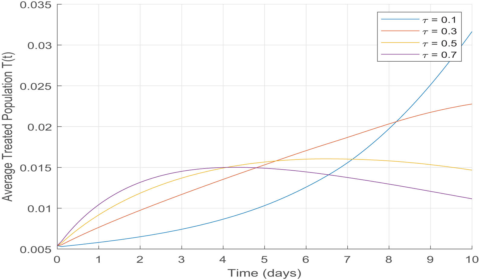
Spatial fragmentation of T ( t , x ) at different treatment rates τ .

4.3 Sensitivity analysis

To perform the sensitivity analysis on the basic reproduction number R 0 of the epidemiological model, we need to calculate the partial derivatives of R 0 with respect to each parameter ( β 1 , β 2 , τ , γ , μ ) and evaluate how changes in each of these parameters influence R 0 . Sensitivity analysis quantifies the responsiveness of R 0 to changes in these parameters [37] (Figure 6).

Figure 6

partial rank correlation coefficient plot depicting the sensitivity analysis of the system’s infection cycle.

Therefore, we have

In summary, the spatio-temporal patterns of the velocities reveal that the velocity component u is influenced by the spatial gradient of S ( t , x ) , v is driven by the spatial gradient of I ( t , x ) , while w is modulated by the gradient of T ( t , x ) . In Figure 3(a), due to the steep slope of S ( t , x ) (indicating a rapid spatial variation), the term − k s ∂ S ∂ x becomes large, resulting in significant changes in u over space and time. Conversely, in regions where S ( t , x ) is nearly constant ( ∂ S ∂ x ≈ 0 ), the velocity u remains relatively stable, leading to a more uniform velocity field.

In Figure 3(b), the large gradient driven by a high infection rate β causes rapid variations in I ( t , x ) , leading to substantial shifts in v . Areas with sharp increases or decreases in infection levels will show notable velocity changes, whereas regions with a more uniform infection spread will exhibit a smoother velocity pattern.

For Figure 3(c), it is important to consider that T ( t , x ) is influenced by its transition dynamics and the treatment rate of I ( t , x ) . Regions with higher treatment rates ( τ ) will significantly affect the gradient of T ( t , x ) , thereby impacting the velocity w . Specifically, w will experience large fluctuations in areas where T undergoes rapid transitions, such as at the boundaries of an outbreak. In contrast, w will be more stable in regions where T changes gradually.

4.4 Contribution to knowledge

This work fundamentally connects epidemiology with fluid dynamics, providing a framework that adeptly models the complex spatio-temporal dynamics of epidemics. Advances in population flow modeling, together with high-resolution numerical methods, create a predictive capability that exceeds traditional epidemic models in capturing the real-world intricacies of disease spread. This approach represents a substantial leap forward in epidemic modeling, supporting more adaptable and spatially targeted public health responses.

The system of PDEs used in this context provides an improved mathematical framework for understanding the dynamics of spatial epidemic propagation. By incorporating specific epidemiological characteristics and the effects of spatial mobility, the equations are designed to model the interactions between susceptible (S), infected (I), and treated (T) population densities. Numerical simulations of these complex interactions can be accurately and stably performed by using third-order Runge-Kutta time integration, in combination with advanced numerical schemes, such as the MUSCL scheme with van Leer slope limiter and the HLLC Riemann solver. This work has contributed to knowledge in the following ways:

• MUSCL scheme with van Leer slope limiter: The scheme MUSCL minimizes the numerical diffusion while preserving stability by improving the spatial resolution of the numerical solution. By stopping oscillations close to steep gradients, the van Leer slope limiter improves this even further and guarantees physical correctness.

• HLLC Riemann solver: For accurate computation of fluxes across cell interfaces, the HLLC Riemann solver is utilized. The solution’s shocks and discontinuities are captured, which is important for simulating abrupt changes in population density during the course of an epidemic.

• Third-order Runge-Kutta time integration: The accuracy and computing efficiency of this temporal integration technique are balanced. Even when the PDEs contain nonlinear elements, it permits steady integration over time.

References

[1] Anderson, D., Tannehill, J. C., Pletcher, R. H., Munipalli, R., & Shankar, V. (2020). Computational fluid mechanics and heat transfer. Boca Raton: CRC Press. DOI: https://doi.org/10.1201/9781351124027-7.10.1201/9781351124027Search in Google Scholar
[2] Arbab, A. I., & Widatallah, H. M. (2010). On the generalized continuity equation. Chinese Physics Letters, 27(8), 084703. DOI: https://doi.org/10.1088/0256-307X/27/8/084703.10.1088/0256-307X/27/8/084703Search in Google Scholar
[3] Attard, P. (2012). Non-equilibrium thermodynamics and statistical mechanics: Foundations and applications. OUP, Oxford. DOI: https://doi.org/10.1093/acprof:oso/9780199662760.003.10.1093/acprof:oso/9780199662760.001.0001Search in Google Scholar
[4] Bagchi, B., Quesne, C., & Znojil, M. (2001). Generalized continuity equation and modified normalization in pt-symmetric quantum mechanics. Modern Physics Letters A, 16(31), 2047–2057. DOI: https://doi.org/10.1142/s0217732301005333.10.1142/S0217732301005333Search in Google Scholar
[5] Balsara, D. S., Dumbser, M., & Abgrall, R. (2014). Multidimensional HLLC Riemann solver for unstructured meshes-with application to Euler and MHD flows. Journal of Computational Physics, 261, 172–208. DOI: https://doi.org/10.1016/j.jcp.2013.12.029.10.1016/j.jcp.2013.12.029Search in Google Scholar
[6] Bertaglia, G., Boscheri, W., Dimarco, G., & Pareschi, L. (2021). Spatial spread of COVID-19 outbreak in Italy using multiscale kinetic transport equations with uncertainty. Mathematical Biosciences and Engineering: MBE, 18(5), 7028–7059. DOI: https://doi.org/10.3934/mbe.2021350.10.3934/mbe.2021350Search in Google Scholar PubMed
[7] Boris, J. P. (1976). Flux-corrected transport modules for solving generalized continuity equations. National Technical Information Service. DOI: https://doi.org/10.1016/b978-0-12-460816-0.50008-7.10.1016/B978-0-12-460816-0.50008-7Search in Google Scholar
[8] Boscarino, S. (2009). On an accurate third-order implicit-explicit Runge-Kutta method for stiff problems. Applied Numerical Mathematics, 59(7), 1515–1528. DOI: https://doi.org/10.1016/j.apnum.2008.10.003.10.1016/j.apnum.2008.10.003Search in Google Scholar
[9] Bourguignon, J.-P., & Brezis, H. (1974). Remarks on the Euler equation. Journal of Functional Analysis, 15(4), 341–363. DOI: https://doi.org/10.1016/0022-1236(74)90027-5.10.1016/0022-1236(74)90027-5Search in Google Scholar
[10] Brauer, F., Castillo-Chavez, C., & Feng, Z. (2019). Mathematical Models in Epidemiology, vol. 69. New York: Springer. DOI: https://doi.org/10.1007/978-1-4939-9828-9_17.10.1007/978-1-4939-9828-9_17Search in Google Scholar
[11] Buebos-Esteve, D. E., & Dagamac, N. H. A. (2024). Spatiotemporal models of dengue epidemiology in the Philippines: Integrating remote sensing and interpretable machine learning. Acta Tropica, 255, 107225. DOI: https://doi.org/10.1016/j.actatropica.2024.107225.10.1016/j.actatropica.2024.107225Search in Google Scholar PubMed
[12] Chen, L., & Schaefer, L. (2018). Godunov-type upwind flux schemes of the two-dimensional finite volume discrete Boltzmann method. Computers and Mathematics with Applications, 75, 3105–3126. DOI: https://doi.org/10.1016/j.camwa.2018.01.034.10.1016/j.camwa.2018.01.034Search in Google Scholar
[13] Cheng, Z., & Wang, J. (2022). Modeling epidemic flow with fluid dynamics. Mathematical Biosciences and Engineering, 19, 8334–8360. DOI: https://doi.org/10.3934/mbe.2022388.10.3934/mbe.2022388Search in Google Scholar PubMed
[14] Cheng, Z., & Wang, J. (2023). A two-phase fluid model for epidemic flow. Infectious Disease Modelling, 8, 920–938. DOI: https://doi.org/10.1016/j.idm.2023.07.001.10.1016/j.idm.2023.07.001Search in Google Scholar PubMed PubMed Central
[15] David, J. F., & Iyaniwura, S. A. (2022). Effect of human mobility on the spatial spread of airborne diseases: An epidemic model with indirect transmission. Bulletin of Mathematical Biology, 84(6), 63. DOI: https://doi.org/10.21203/rs.3.rs-965234/v1.10.1007/s11538-022-01020-8Search in Google Scholar PubMed PubMed Central
[16] Duran, I., & Moreau, S. (2013). Solution of the quasi-one-dimensional linearized Euler equations using flow invariants and the Magnus expansion. Journal of Fluid Mechanics, 723, 190–231. DOI: https://doi.org/10.1017/jfm.2013.118.10.1017/jfm.2013.118Search in Google Scholar
[17] Elliott, P., & Wartenberg, D. (2004). Spatial epidemiology: current approaches and future challenges. Environmental health perspectives, 112(9), 998–1006. DOI: https://doi.org/10.1289/ehp.6735.10.1289/ehp.6735Search in Google Scholar PubMed PubMed Central
[18] Ferraccioli, F., Stilianakis, N. I., & Veliov, V. M. (2024). A spatial epidemic model with contact and mobility restrictions. Mathematical and Computer Modelling of Dynamical Systems, 30, 284–302. DOI: https://doi.org/10.1080/13873954.2024.2341693.10.1080/13873954.2024.2341693Search in Google Scholar
[19] Fosu, G. O., Akweittey, E., & Adu-Sackey, A. (2020). Next-generation matrices and basic reproductive numbers for all phases of the coronavirus disease. Gabriel Obed Fosu, Emmanuel Akweittey, and Albert Adu-Sackey. Next-generation matrices and basic reproductive numbers for all phases of the coronavirus disease. Open Journal of Mathematical Sciences, 4(1), 261–272. DOI: https://doi.org/10.2139/ssrn.3595958.10.30538/oms2020.0117Search in Google Scholar
[20] Giles, M. B., & Pierce, N. A. (2001). Analytic adjoint solutions for the quasi-one-dimensional Euler equations. Journal of Fluid Mechanics, 426, 327–345. DOI: https://doi.org/10.1017/s0022112000002366.10.1017/S0022112000002366Search in Google Scholar
[21] Godunov, S. K., & Bohachevsky, I. (1959). Finite difference method for numerical computation of discontinuous solutions of the equations of fluid dynamics. Matematičeskij sbornik, 47(89)(3), 271–306. DOI: https://hal.science/hal-01620642/file/SG1959.pdf.Search in Google Scholar
[22] Gosse, L. (2014). A two-dimensional version of the Godunov scheme for scalar balance laws. SIAM Journal on Numerical Analysis, 52(2), 626–652. DOI: https://doi.org/10.1137/130925906.10.1137/130925906Search in Google Scholar
[23] Gouin, H., & Gavrilyuk, S. (1999). Hamilton’s principle and Rankine-Hugoniot conditions for general motions of mixtures. Meccanica, 34, 39–47. DOI: https://doi.org/10.1023/A:1004370127958.10.1023/A:1004370127958Search in Google Scholar
[24] Green, P. J., Hjort, N. L., & Richardson, S. (2003). Highly Structured Stochastic Systems, vol. 27. Oxford: Oxford University Press. DOI: https://doi.org/10.1093/oso/9780198510550.003.0001.10.1093/oso/9780198510550.001.0001Search in Google Scholar
[25] Hou, J., Liang, Q., Zhang, H., & Hinkelmann, R. (2014). Multislope MUSCL method applied to solve shallow water equations. Computers and Mathematics with Applications, 68, 2012–2027. DOI: https://doi.org/10.1016/j.camwa.2014.09.018.10.1016/j.camwa.2014.09.018Search in Google Scholar
[26] Hou, J., Liang, Q., Zhang, H., & Hinkelmann, R. (2015). An efficient unstructured MUSCL scheme for solving the 2D shallow water equations. Environmental Modelling and Software, 66, 131–152. DOI: https://doi.org/10.1016/j.envsoft.2014.12.007.10.1016/j.envsoft.2014.12.007Search in Google Scholar
[27] Hou, J., Simons, F., Mahgoub, M., & Hinkelmann, R. (2013). A robust well-balanced model on unstructured grids for shallow water flows with wetting and drying over complex topography. Computer Methods in Applied Mechanics and Engineering, 257, 126–149. DOI: https://www.sciencedirect.com/science/article/pii/S0045782513000339.10.1016/j.cma.2013.01.015Search in Google Scholar
[28] Jaisankar, S., & Rao, S. R. (2009). A central Rankine-Hugoniot solver for hyperbolic conservation laws. Journal of Computational Physics, 228(3), 770–798. DOI: https://doi.org/10.1016/j.jcp.2008.10.002.10.1016/j.jcp.2008.10.002Search in Google Scholar
[29] Kessels, F. V. W., van Lint, H., Vuik, K., & Hoogendoorn, S. (2015). Genealogy of traffic flow models. EURO Journal on Transportation and Logistics, 4, 445–473. DOI: https://doi.org/10.1007/s13676-014-0045-5.10.1007/s13676-014-0045-5Search in Google Scholar
[30] Koçak, H., & Pinar, Z. (2022). Wave propagations for dispersive variants of spatial models in epidemiology and ecology. Communications in Nonlinear Science and Numerical Simulation, 109, 106316. DOI: https://doi.org/10.1016/j.cnsns.2022.106316.10.1016/j.cnsns.2022.106316Search in Google Scholar
[31] Sweby, K. (1999). Godunov Methods. . In Toro, E. F., editor. Godunov Methods. New York: Springer. DOI: https://doi.org/10.1007/978-1-4615-0663-8_85.10.1007/978-1-4615-0663-8_85Search in Google Scholar
[32] Langtangen, H. P. (2016). Solving nonlinear ODE and PDE problems. Center for Biomedical Computing, Simula Research Laboratory and Department of Informatics, University of Oslo, Oslo, Norway. http://hplgit.github.io/INF5620/doc/pub/H14/nonlin/pdf/main_nonlin-4print-A4-2up.pdf. Search in Google Scholar
[33] Laugier, A., & Garai, J. (2007). Derivation of the ideal gas law. Journal of Chemical Education, 84(11), 1832. DOI: https://doi.org/10.1021/ed084p1832.10.1021/ed084p1832Search in Google Scholar
[34] Li, J., Xiang, T., & He, L. (2021). Modeling epidemic spread in transportation networks: A review. Journal of Traffic and Transportation Engineering, 8, 139–152. DOI: https://doi.org/10.1016/j.jtte.2020.10.003.10.1016/j.jtte.2020.10.003Search in Google Scholar
[35] Lin, X.-B. (2000). Generalized Rankine-Hugoniot condition and shock solutions for quasilinear hyperbolic systems. Journal of Differential Equations, 168(2), 321–354. DOI: https://doi.org/10.1006/jdeq.2000.3889.10.1006/jdeq.2000.3889Search in Google Scholar
[36] Lloyd, A. L., & May, R. M. (1996). Spatial heterogeneity in epidemic models. Journal of Theoretical Biology, 179(1), 1–11. DOI: https://doi.org/10.1006/jtbi.1996.0042.10.1006/jtbi.1996.0042Search in Google Scholar PubMed
[37] Lu, X., & Borgonovo, E. (2023). Global sensitivity analysis in epidemiological modeling. European Journal of Operational Research, 304(1), 9–24. DOI: https://doi.org/10.1016/j.ejor.2021.11.018.10.1016/j.ejor.2021.11.018Search in Google Scholar PubMed PubMed Central
[38] Mahsin, M., Deardon, R., & Brown, P. (2022). Geographically dependent individual-level models for infectious diseases transmission. Biostatistics, 23(1), 1–17. DOI: https://doi.org/10.1093/biostatistics/kxaa009.10.1093/biostatistics/kxaa009Search in Google Scholar PubMed
[39] Mvogo, A., Tiomela, S. A., Macías-Díaz, J. E., & Bertrand, B. (2023). Dynamics of a cross-superdiffusive SIRS model with delay effects in transmission and treatment. Nonlinear Dynamics, 111(14), 13619–13639. DOI: https://doi.org/10.1007/s11071-023-08530-7.10.1007/s11071-023-08530-7Search in Google Scholar PubMed PubMed Central
[40] Nikitin, N. (2006). Third-order-accurate semi-implicit Runge-Kutta scheme for incompressible Navier-stokes equations. International Journal for Numerical Methods in Fluids, 51(2), 221–233. DOI: https://doi.org/10.1002/fld.1122.10.1002/fld.1122Search in Google Scholar
[41] Ostfeld, R. S., Glass, G. E., & Keesing, F. (2005). Spatial epidemiology: an emerging (or re-emerging) discipline. Trends in Ecology & Evolution, 20(6), 328–336. DOI: https://doi.org/10.1016/j.tree.2005.03.009.10.1016/j.tree.2005.03.009Search in Google Scholar PubMed
[42] Pan, R., & Zhu, Y. (2016). Singularity formation for one dimensional full Euler equations. Journal of Differential Equations, 261(12), 7132–7144. DOI: https://doi.org/10.1016/j.jde.2016.09.015.10.1016/j.jde.2016.09.015Search in Google Scholar
[43] Pereira, M., Kulcsár, B., Lipták, G., Kovacs, M., & Szederkényi, G. (2024). The traffic reaction model: a kinetic compartmental approach to road traffic modeling. Transportation Research Part C: Emerging Technologies, 158, e104435–e104435. DOI: https://doi.org/10.1016/j.trc.2023.104435.10.1016/j.trc.2023.104435Search in Google Scholar
[44] Perrot, P. (1998). A to Z of Thermodynamics. OUP, Oxford. DOI: https://doi.org/10.1093/oso/9780198565567.001.0001.10.1093/oso/9780198565567.001.0001Search in Google Scholar
[45] Pletcher, R. H., Tannehill, J. C., & Anderson, D. (2012). Computational Fluid Mechanics and Heat Transfer. Boca Raton: CRC Press. DOI: https://doi.org/10.1016/0142-727x(86)90038-x.10.1016/0142-727X(86)90038-XSearch in Google Scholar
[46] Pujante-Otalora, L., Canovas-Segura, B., Campos, M., & Juarez, J. M. (2023). The use of networks in spatial and temporal computational models for outbreak spread in epidemiology: A systematic review. Journal of Biomedical Informatics, 143, 104422. DOI: https://doi.org/10.1016/j.jbi.2023.104422.10.1016/j.jbi.2023.104422Search in Google Scholar PubMed
[47] Richardson, S. (2003). Spatial models in epidemiological applications. Oxford Statistical Science Series, pp. 237–259. Oxford: Oxford University Press. DOI: https://doi.org/10.1093/oso/9780198510550.003.0023. 10.1093/oso/9780198510550.003.0023Search in Google Scholar
[48] Ruan, S. (2007). Spatial-temporal dynamics in nonlocal epidemiological models. In: Mathematics for life science and medicine, pp. 97–122. Berlin, Heidelberg: Springer Berlin Heidelberg. DOI: https://doi.org/10.1007/978-3-540-34426-1_5.10.1007/978-3-540-34426-1_5Search in Google Scholar
[49] Salman, A. M., Mohd, M. H., & Muhammad, A. (2023). A novel approach to investigate the stability analysis and the dynamics of reaction-diffusion SVIR epidemic model. Communications in Nonlinear Science and Numerical Simulation, 126, 107517. DOI: https://doi.org/10.1016/j.cnsns.2023.107517.10.1016/j.cnsns.2023.107517Search in Google Scholar
[50] Samsuzzoha, M., Singh, M., & Lucy, D. (2013). Uncertainty and sensitivity analysis of the basic reproduction number of a vaccinated epidemic model of influenza. Applied Mathematical Modelling, 37(3), 903–915. DOI: https://doi.org/10.1016/j.apm.2012.03.029.10.1016/j.apm.2012.03.029Search in Google Scholar
[51] Simon, S., & Mandal, J. (2019). A simple cure for numerical shock instability in the HLLC Riemann solver. Journal of Computational Physics, 378, 477–496. DOI: https://doi.org/10.1016/j.jcp.2018.11.022.10.1016/j.jcp.2018.11.022Search in Google Scholar
[52] Tiomela, S. A., Macías-Díaz, J. E., & Mvogo, A. (2021). Computer simulation of the dynamics of a spatial susceptible-infected-recovered epidemic model with time delays in transmission and treatment. Computer Methods and Programs in Biomedicine, 212, 106469. DOI: https://doi.org/10.1016/j.cmpb.2021.106469.10.1016/j.cmpb.2021.106469Search in Google Scholar PubMed
[53] Tsatsaris, A., Kalogeropoulos, K., & Stathopoulos, N. (2023). Chapter 1 - geoinformatics, spatial epidemiology, and public health. In Stathopoulos, N., Tsatsaris, A., & Kalogeropoulos, K., editors, Geoinformatics for Geosciences, Earth Observation, pp. 3–29. Amsterdam, The Netherlands: Elsevier. DOI: https://doi.org/10.1016/b978-0-323-98983-1.00002-8.10.1016/B978-0-323-98983-1.00002-8Search in Google Scholar
[54] Tschoegl, N. W. (2000). Fundamentals of equilibrium and steady-state thermodynamics. Amsterdam, The Netherlands: Elsevier. DOI: https://doi.org/10.1016/b978-0-444-50426-5.50046-x.10.1016/B978-0-444-50426-5.50046-XSearch in Google Scholar
[55] Tsori, Y., & Granek, R. (2021). Epidemiological model for the inhomogeneous spatial spreading of covid-19 and other diseases. PloS one, 16(2), e0246056. DOI: https://doi.org/10.1371/journal.pone.0246056.10.1371/journal.pone.0246056Search in Google Scholar PubMed PubMed Central
[56] van Leer, B. (2011). A historical oversight: Vladimir P. Kolgan and his high-resolution scheme. Journal of Computational Physics, 230(7), 2378–2383. DOI: https://doi.org/10.1016/j.jcp.2010.12.032.10.1016/j.jcp.2010.12.032Search in Google Scholar
[57] van Wageningen-Kessels, F., Daamen, W., & Hoogendoorn, S. P. (2018). Two-dimensional approximate Godunov scheme and what it means for continuum Pedestrian flow models. Transportation Science, 52(3), 547–563. DOI: https://doi.org/10.1287/trsc.2017.0793.10.1287/trsc.2017.0793Search in Google Scholar
[58] Vazquez, R., & Krstic, M. (2008). Control of 1D parabolic PDEs with Volterra nonlinearities, part i: Design. Automatica, 44(11), 2778–2790. DOI: https://doi.org/10.1016/j.automatica.2008.04.013.10.1016/j.automatica.2008.04.013Search in Google Scholar
[59] Wang, Y., Yu, X., Guo, J., Papamichail, I., Papageorgiou, M., Zhang, L., Hu, S., Li, Y., & Sun, J. (2022). Macroscopic traffic flow modelling of large-scale freeway networks with field data verification: State-of-the-art review, benchmarking framework, and case studies using metanet. Transportation Research Part C: Emerging Technologies, 145, 103904. DOI: https://doi.org/10.1016/j.trc.2022.103904.10.1016/j.trc.2022.103904Search in Google Scholar
[60] Wendroff, B. (1999). A two-dimensional HLLE Riemann solver and associated Godunov-type difference scheme for gas dynamics. Computers & Mathematics with Applications, 38, 175–185. DOI: https://doi.org/10.1016/s0898-1221(99)00296-5.10.1016/S0898-1221(99)00296-5Search in Google Scholar
[61] Wood, S. M., Alston, L., Beks, H., Mc Namara K., Coffee N., Clark R. A., Wong Shee A., & Versace V. L. (2023). Quality appraisal of spatial epidemiology and health geography research: A scoping review of systematic reviews. Health & Place, 83, 103108. DOI: https://doi.org/10.1016/j.healthplace.2023.103108.10.1016/j.healthplace.2023.103108Search in Google Scholar PubMed
[62] Woody, A. I. (2013). How is the ideal gas law explanatory? Science & Education, 22, 1563–1580. DOI: https://doi.org/10.1007/s11191-011-9424-6.10.1007/s11191-011-9424-6Search in Google Scholar
[63] Yang, H. M. (2014). The basic reproduction number obtained from Jacobian and next generation matrices-a case study of dengue transmission modelling. Biosystems, 126, 52–75. DOI: https://doi.org/10.1016/j.biosystems.2014.10.002.10.1016/j.biosystems.2014.10.002Search in Google Scholar PubMed
[64] Yeddula, S. R., Guzmán-Iñigo, J., & Morgans, A. S. (2022). A solution for the quasi-one-dimensional linearised Euler equations with heat transfer. Journal of Fluid Mechanics, 936, R3. DOI: https://doi.org/10.1017/jfm.2022.101.10.1017/jfm.2022.101Search in Google Scholar
[65] Zeng, X. (2016). A general approach to enhance slope limiters in MUSCL schemes on nonuniform rectilinear grids. SIAM Journal on Scientific Computing, 38(2), A789–A813. DOI: https://doi.org/10.1137/140970185.10.1137/140970185Search in Google Scholar
[66] Zhang, Q., & Shu, C.-W. (2010). Stability analysis and a priori error estimates of the third-order explicit Runge-Kutta discontinuous Galerkin method for scalar conservation laws. SIAM Journal on Numerical Analysis, 48(3), 1038–1063. DOI: https://doi.org/10.1137/090771363.10.1137/090771363Search in Google Scholar
[67] Zhuang, Q., & Wang, J. (2021). A spatial epidemic model with a moving boundary. Infectious Disease Modelling, 6, 1046–1060. DOI: https://doi.org/10.1016/j.idm.2021.08.005.10.1016/j.idm.2021.08.005Search in Google Scholar PubMed PubMed Central
© 2024 the author(s), published by De Gruyter
This work is licensed under the Creative Commons Attribution 4.0 International License.
Articles in the same Issue
- Special Issue: Recent Trends in Mathematical Biology – Theory, Methods, and Applications
- Editorial for the Special Issue: Recent trends in mathematical Biology – Theory, methods, and applications
- Behavior of solutions of a discrete population model with mutualistic interaction
- Influence of media campaigns efforts to control spread of COVID-19 pandemic with vaccination: A modeling study
- Optimal control and bifurcation analysis of SEIHR model for COVID-19 with vaccination strategies and mask efficiency
- A mathematical study of the adrenocorticotropic hormone as a regulator of human gene expression in adrenal glands
- On building machine learning models for medical dataset with correlated features
- Analysis and numerical simulation of fractional-order blood alcohol model with singular and non-singular kernels
- Stability and bifurcation analysis of a nested multi-scale model for COVID-19 viral infection
- Augmenting heart disease prediction with explainable AI: A study of classification models
- Plankton interaction model: Effect of prey refuge and harvesting
- Modelling the leadership role of police in controlling COVID-19
- Robust H∞ filter-based functional observer design for descriptor systems: An application to cardiovascular system monitoring
- Regular Articles
- Mathematical modelling of COVID-19 dynamics using SVEAIQHR model
- Optimal control of susceptible mature pest concerning disease-induced pest-natural enemy system with cost-effectiveness
- Correlated dynamics of immune network and sl(3, R) symmetry algebra
- Variational multiscale stabilized FEM for cardiovascular flows in complex arterial vessels under magnetic forces
- Assessing the impact of information-induced self-protection on Zika transmission: A mathematical modeling approach
- An analysis of hybrid impulsive prey-predator-mutualist system on nonuniform time domains
- Modelling the adverse impacts of urbanization on human health
- Markov modeling on dynamic state space for genetic disorders and infectious diseases with mutations: Probabilistic framework, parameter estimation, and applications
- In silico analysis: Fulleropyrrolidine derivatives against HIV-PR mutants and SARS-CoV-2 Mpro
- Tangleoids with quantum field theories in biosystems
- Analytic solution of a fractional-order hepatitis model using Laplace Adomian decomposition method and optimal control analysis
- Effect of awareness and saturated treatment on the transmission of infectious diseases
- Development of Aβ and anti-Aβ dynamics models for Alzheimer’s disease
- Compartmental modeling approach for prediction of unreported cases of COVID-19 with awareness through effective testing program
- COVID-19 transmission dynamics in close-contacts facilities: Optimizing control strategies
- Modeling and analysis of ensemble average solvation energy and solute–solvent interfacial fluctuations