Plankton interaction model: Effect of prey refuge and harvesting

Poulomi Basak; Satish Kumar Tiwari; Jai Prakash Tripathi; Vandana Tiwari; Ratnesh Kumar Mishra

doi:10.1515/cmb-2024-0011

Article Open Access

Plankton interaction model: Effect of prey refuge and harvesting

Poulomi Basak , Satish Kumar Tiwari , Jai Prakash Tripathi , Vandana Tiwari and Ratnesh Kumar Mishra

Published/Copyright: September 30, 2024

Published by

Become an author with De Gruyter Brill

Submit Manuscript Author Information

From the journal Computational and Mathematical Biophysics Volume 12 Issue 1

Abstract

Harmful algal blooms are one of the major threats to aquatic ecosystem. Some phytoplankton species produce toxins during algal bloom and affect other aquatic species as well as human beings. Thus, for the conservation of aquatic habitat, it is much needed to control such phenomenon. In the present study, we propose a mathematical model of toxin-producing phytoplankton and zooplankton species, which follows the Holling Type III functional response. We consider the effect of prey refuge and harvesting on both the species. Boundedness of the proposed model, existence of equilibria, and their stability have been discussed analytically. We also discuss the optimal harvesting policy and existence of bionomic equilibrium. The numerical simulation has also been performed. We identify the control parameters that are responsible for the system dynamics of the model. The parameter prey refuge has a great impact on the dynamics of the model system. Higher value of prey refuge leads to the stable dynamics. Also, the growth rate of phytoplankton acts as a control parameter for the dynamics of the model. The higher value of growth rate of phytoplankton is responsible for oscillatory behavior.

Keywords: optimal harvesting policy; stability analysis; harmful algal blooms; prey refuge; bionomic equilibrium

MSC 2010: 92B10; 37N25; 92B05

1 Introduction

Planktons are the main supplier of dissolved oxygen in water and play an important role in the food chain of aquatic ecosystem [13]. Harmful algal blooms (HABs) are one of the major causes of the degradation of aquatic biodiversity. Human health, fisheries, and local economies are also affected by this global problem, “Harmful Algal Blooms” [23]. HABs occur when an algae population (e.g., Dinoflagellates) experiences explosive growth and releases toxins or has other negative effects on the environment [5]. River Ganga is one of the most significant rivers in India and provides the habitat to numerous aquatic species and microorganisms. However, the color of the river Ganga suddenly changed to green due to the rise of algal bloom in the Varanasi and the nearby regions during May–June 2021 [3]. Thus, the conservation of aquatic diversity from such threats is much needed for ecological as well as economical points of view. Many authors have developed different mathematical models addressing the issue of HABs and suggested proper management for biodiversity conservation [6–9,20–22]. Chattopadhayay et al. [8] observed that toxic substances released by toxin-producing phytoplankton (TPP) play a significant role in the termination of planktonic blooms. As a result, toxic chemicals serve as a biocontrol agent for other plankton species. A three-species model was studied by Roy and Chattopadhyay [21], and the authors observed that toxic or allelopathic compounds produced by TPP may assist in diminishing the competition coefficient among various phytoplankton species. Chakraborty et al. [6] developed a model with three interacting species, taking into account the impact of avoidance of zooplankton for the toxic phytoplankton in the presence of a non-toxic one. It has been noted that high avoidance plays a crucial role in facilitating the coexistence of toxic phytoplankton, non-toxic phytoplankton and zooplankton. A mathematical model of HABs was studied by Braselton and Braselton [5], and the authors have suggested that introducing additional prey or predators of the original predator may assist in its control. Sarkar et al. [22] studied the effect of HABs on zooplankton species due to TPP through a food chain model among TPP and zooplankton species. A three-species plankton model with optimal control strategy has been studied by Xiang et al. [29].

The dynamical behavior of toxic phytoplankton and zooplankton model with the impact of phytoplankton harvesting was analyzed by Zhang and Niu [30]. The authors found that phytoplankton and zooplankton populations oscillate periodically when the harvesting level is high. Li et al. [14] developed a phytoplankton–zooplankton interaction model with toxin effect and refuge. The authors suggested that when making decisions regarding predation and control of HABs in aquatic system, the toxin and refuge have a great impact. Pandey et al. [17] constructed and examined a stage-structured prey-predator model that incorporates refuge behavior for prey and gestational delay. The authors have shown that the immature prey refuge functions as a destabilizing factor in the system in the absence of time delay while it serves as a control parameter in the presence of delay. The detailed recent studies related to prey refuge can also be found in [25–27]. An optimal control of harvesting effort in phytoplankton-zooplankton model with the effect of toxicity was discussed by Agnihotri and Kaur [2]. Huda et al. [12] investigated the dynamic behavior of a prey-predator model in which harvesting effort is employed as a control variable. Their study revealed that the optimal solution can lead to the achievement of ecosystem sustainability. Panja et al. [18] suggested that for the stability of ecological system, we should control the environmental toxins released by natural or different human activities through a plankton-fish model with toxicant and harvesting. Lv et al. [15] studied the effect of harvesting on plankton dynamics and found that the zero discounting leads to the maximization of economic revenue and that an infinite discount rate leads to complete dissipation of economic rent. The effect of linear harvesting along with the Allee effect in a delayed phytoplankton zooplankton model was discussed by Meng et al. [16], and the authors obtained optimal harvesting policy using Pontryagin’s maximum principle. Recently, Agmour et al. [1] developed a mathematical model among the dinoflagellate phytoplankton and mytilid species with effect of harvesting in both the species and analyzed the bionomic equilibrium and optimal harvesting policy for their proposed model. In this article, we propose a mathematical model of the interaction of phytoplankton and zooplankton influenced by toxin release by phytoplankton. We also consider the impact of harvesting on both the species in the present model. The main objective of this article is to study the dynamics of the proposed model analytically as well as numerically.

The present article has been organized as follows. In Section 2, a two-species phytoplankton-zooplankton model is presented. The mathematical analysis and optimal harvesting policy are discussed in Section 3. Results of numerical simulations are presented and discussed in Section 4. Finally, Section 5 concludes the study.

2 Model formulation

In this study, we propose a mathematical model to elucidate the dynamics of phytoplankton and zooplankton populations. We consider the impact of toxins released by phytoplankton, which affects the zooplankton species. We assume that the interaction among the plankton species follows the Holling type-III functional response. As the liberation of toxin reduces the growth of zooplankton, it causes substantial mortality of zooplankton. During the toxin liberation period, TPP is not easily accessible; hence, a more common and intuitive choice may be the Holling type II or type III functional response to describe the grazing phenomena [8]. Holling [10] proposed Holling type-III function response of the form

w 1 u 2 c + u 2 .

Here, u is the phytoplankton population density. In the present model, we incorporate refuge protecting m u of phytoplankton, where m ∈ [ 0 , 1 ) . Therefore, ( 1 − m ) u prey is only available for predators. We also consider harvesting in phytoplankton and zooplankton. Considering above discussion and following [1,11,14], the present model is described via the following set of differential equations:

(1) d u d t = a u − b u 2 − ( 1 − m ) 2 β u 2 v ( 1 − m ) 2 u 2 + D 2 − q 1 e u , d v d t = − δ v + α β ( 1 − m ) 2 u 2 v ( 1 − m ) 2 u 2 + D 2 − γ u v 2 − q 2 e v ,

with initial condition

(2) u ( 0 ) = u 0 > 0 , v ( 0 ) = v 0 > 0 .

Here, u denotes the density of phytoplankton and v denotes the density of the zooplankton population at any time t . Parameter a is the intrinsic growth rate of phytoplankton. Parameter b is the phytoplankton mortality rate due to intraspecific competition. Parameter m is the coefficient of refuge. Parameter β represents the phytoplankton uptake rate by zooplankton, and D is the saturation constant. δ is the death rate of zooplankton. Parameters α and γ are the conversion coefficient and rate of toxin released by phytoplankton, respectively. The term γ v 2 denotes the functional response of phytoplankton to the density of zooplankton, and it comes through the production of toxic substances by phytoplankton. q 1 and q 2 are the catchability coefficients for the phytoplankton and zooplankton, respectively. Parameter e represents the combined harvesting fishing efforts of phytoplankton and zooplankton.

3 Mathematical analysis of model system

Lemma 1

R + 2 is invariant for the model system (1) and all the solutions of system (1) that initiates in the interior of the positive quadrant will be attracted to the set Λ = ( u , v ) ∈ R + 2 : 0 ≤ u ≤ a b , u + v α ≤ ( a + δ ) 2 4 δ b .

Proof

Obviously, the solution of ( 1 ) with positive initial conditions remains positive.

From the first equation of system ( 1 ) , it is clear that d u d t ≤ a u − b u 2 .

Then, by the standard comparison theorem, it can be shown that

lim t → ∞ sup u ( t ) ≤ a b .

Let us define a function w = u + v α .

The time derivative of w along the solutions of ( 1 ) is

d w d t = d u d t + 1 α d v d t = a u − b u 2 − q 1 e u − δ v α − γ u v 2 α − q 2 e v α d w d t ≤ a u − b u 2 − δ v α = ( a u − b u 2 + δ u ) − δ w .

Now, we have

d w d t + δ w ≤ ( a + δ ) 2 4 b .

By applying the theory of Birkhoff and Rota [4] of differential inequality, we obtain

0 < w ( u , v ) ≤ ( a + δ ) 2 4 δ b ( 1 − e − δ t ) + w ( u ( 0 ) , v ( 0 ) ) e − δ t .

When t tends to the infinity, we have 0 < w ( u , v ) ≤ ( a + δ ) 2 4 δ b .□

3.1 Existence of equilibrium points and their local stability

In this section, we delve into the examination of the existence and stability of equilibrium points to analyze the dynamics of the temporal model (1).

The equilibrium points of the system (1) are as follows:

The trivial equilibrium point E 0 = ( 0 , 0 ) , which always exists.
The zooplankton-free equilibrium point E 1 = ( u 1 , 0 ) , where u 1 = a − q 1 e b . E 1 exists if a > q 1 e .
The coexistence equilibrium point E * = ( u * , v * ) is the positive solution of the following equations:
(3) a − b u * − ( 1 − m ) 2 β u * v * ( 1 − m ) 2 u * 2 + D 2 − q 1 e = 0

(4) − δ + α β ( 1 − m ) 2 u * 2 ( 1 − m ) 2 u * 2 + D 2 − γ u * v * − q 2 e = 0 .

u * and v * are the positive solutions of the equations in equation (3) and (4). It is difficult to find the value of u * and v * in terms of parameters. Thus, we have shown the existence of nontrivial equilibrium point E * ( u * , v * ) by taking the following suitable numerical values of involved parameters:

(5) a = 0.9 , b = 0.5 , m = 0.8 , β = 1.5 , D = 0.1 , q 1 = 0.2 , e = 0.4 , δ = 0.6 , α = 0.7 , γ = 0.05 , q 2 = 0.08 .

Figure 1 shows the existence of equilibrium point E * ( u * , v * ) as one can see that at the set of parameter values given in equation (5), we have E * ( u * , v * ) = ( 0.63 , 0.35 ) .

$Figure 1 Existence of interior equilibrium point E * ( u * , v * ) {E}^{* }\left({u}^{* },{v}^{* }) of model system (1).$

Figure 1

Existence of interior equilibrium point E * ( u * , v * ) of model system (1).

3.2 Stability analysis

The Jacobian matrix of model system (1) at E 0 = ( 0 , 0 ) is
J ( E 0 ) = a − q 1 e 0 0 − δ − q 2 e .
The eigenvalues of J ( E 0 ) are a − q 1 e and − δ − q 2 e . Thus, the trivial equilibrium point E 0 exhibits local asymptotic stability when the condition e > a q 1 is satisfied.
The Jacobian matrix of model system (1) at E 1 = ( u 1 , 0 ) is
J ( E 1 ) = − b u 1 − ( 1 − m ) 2 β u 1 2 ( 1 − m ) 2 u 1 2 + D 2 0 − δ + α β ( 1 − m ) 2 u 1 2 ( 1 − m ) 2 u 1 2 + D 2 − q 2 e .
The eigenvalues of J ( E 1 ) are − b u 1 and − δ + α β ( 1 − m ) 2 u 1 2 ( 1 − m ) 2 u 1 2 + D 2 − q 2 e . Thus, the equilibrium point E 1 is stable if e > 1 q 2 α β ( 1 − m ) 2 u 1 2 ( 1 − m ) 2 u 1 2 + D 2 − δ .
The Jacobian matrix corresponding to E * ( u * , v * ) is given by
J ( E * ) = j 11 j 12 j 21 j 22 ,
where
j 11 = u * − b + ( 1 − m ) 4 u * 2 β v * − D 2 ( 1 − m ) 2 β v * ( ( 1 − m ) 2 u * 2 + D 2 ) 2 , j 12 = − ( 1 − m ) 2 β u * 2 ( 1 − m ) 2 u * 2 + D 2 , j 21 = 2 D 2 α β ( 1 − m ) 2 u * v * ( ( 1 − m ) 2 u * 2 + D 2 ) 2 − γ v * 2 , j 22 = − γ u * v * .
The characteristic equation of the above matrix is given by
λ 2 − B 1 λ + B 2 = 0 ,
where B 1 = j 11 + j 22 and B 2 = j 11 j 22 − j 12 j 21 .

Theorem 1

The equilibrium point E * ( u * , v * ) is locally asymptotically stable if the following conditions hold:

( 1 − m ) 2 u * 2 < D 2 ,
2 D 2 α β ( 1 − m ) 2 u * ( ( 1 − m ) 2 u * 2 + D 2 ) 2 > γ v * .

Proof

Using Routh-Hurwitz criterion, equilibrium point E * ( u * , v * ) is locally asymptotically stable if,

(i) Trace of J ( E * ) = j 11 + j 22 = B 1 = u * − b + ( 1 − m ) 4 u * 2 β v * − D 2 ( 1 − m ) 2 β v * ( ( 1 − m ) 2 u * 2 + D 2 ) 2 − γ u * v * < 0 ⇒ ( 1 − m ) 2 u * 2 < D 2 ,

□ (ii) Determinant of J ( E * ) = j 11 j 22 − j 12 j 21 = B 2 > 0 ⇒ j 12 j 21 < 0 ⇒ j 21 > 0 ⇒ 2 D 2 α β ( 1 − m ) 2 u * ( ( 1 − m ) 2 u * 2 + D 2 ) 2 > γ v * .

3.3 Bionomic equilibrium and optimal harvesting policy

In this section, we explore the concept of bionomic equilibrium and the optimal harvesting policy. Bionomic equilibrium is the combination of biological equilibrium and economic equilibrium. The bionomic equilibrium is a concept that integrates biological and economical aspects in the population dynamics. The biological equilibrium is found by solving the equations d u d t = 0 and d v d t = 0 simultaneously. Economic equilibrium is obtained when the total revenue (TR) obtained by selling the harvested biomass is equal to the total cost (TC) of harvesting the biomass. Also, we have discussed the optimal harvesting policy by constructing an appropriate Hamiltonian function and using Pontryagin’s maximum principle [19] for the model system (1).

3.3.1 Bionomic equilibrium

The net economic revenue at time t is given by

π ( u , v , e , t ) = p 1 q 1 e u + p 2 q 2 e v − c e ,

where p 1 is the constant price per biomass of phytoplankton, p 2 is the constant price per biomass of zooplankton, and c is the fishing cost per unit effort.

Now, we have

(6) d u d t = 0 ⇒ e = 1 q 1 a − b u − ( 1 − m ) 2 β u v ( 1 − m ) 2 u 2 + D 2 ,

(7) d v d t = 0 ⇒ e = 1 q 2 − δ + α β ( 1 − m ) 2 u 2 ( 1 − m ) 2 u 2 + D 2 − γ u v .

From equations (6) and (7), the following equation represents the non-trivial equilibrium solution that occurs at a point on the biological equilibrium curve:

(8) 1 q 1 a − b u − ( 1 − m ) 2 β u v ( 1 − m ) 2 u 2 + D 2 − 1 q 2 − δ + α β ( 1 − m ) 2 u 2 ( 1 − m ) 2 u 2 + D 2 − γ u v = 0 .

Thus, from equation (8), the bionomic equilibrium P ∞ ( u ∞ , v ∞ ) of the open-access fishery (i.e., π = 0 ) is given by v ∞ = c − p 1 q 1 u ∞ p 2 q 2 , where u ∞ is the positive root of the following equation:

(9) λ 4 u 4 + λ 3 u 3 + λ 2 u 2 + λ 1 u + λ 0 = 0 ,

where

λ 4 = γ p 1 q 1 ( 1 − m ) 2 p 2 q 2 2 , λ 3 = ( 1 − m ) 2 ( b p 2 q 2 2 − γ c q 1 ) p 2 q 1 q 2 2 , λ 2 = ( 1 − m ) 2 p 2 q 2 ( − a q 2 − δ q 1 + α β q 1 ) + p 1 q 1 ( γ q 1 D 2 − ( 1 − m ) 2 β q 2 ) p 2 q 1 q 2 2 , λ 1 = q 2 ( b D 2 p 2 q 2 + c ( 1 − m ) 2 β ) − γ c D 2 q 1 p 2 q 1 q 2 2 , λ 0 = − D 2 ( a q 2 + δ q 1 ) q 1 q 2 .

Equation (9) has unique positive root u ∞ if

b p 2 q 2 2 > γ c q 1 , α β q 1 > a q 2 + δ q 1 ,
γ q 1 D 2 > ( 1 − m ) 2 β q 2 , q 2 ( b D 2 p 2 q 2 + c ( 1 − m ) 2 β ) > γ c D 2 q 1 .

3.3.2 Optimal harvesting policy

The objective function that we optimize is given by

J = ∫ 0 + ∞ π ( u , v , e , t ) exp − ε t d t = ∫ 0 + ∞ [ ( p 1 q 1 u + p 2 q 2 v − c ) e ] exp − ε t d t ,

where ε represents the instantaneous annual rate of discount.

The associated Hamiltonian function is

(10) H = exp − ε t ( p 1 q 1 u + p 2 q 2 v − c ) e + ϱ 1 [ a u − b u 2 − ( 1 − m ) 2 β u 2 v ( 1 − m ) 2 u 2 + D 2 − q 1 e u ] + ϱ 2 [ − δ v + α β ( 1 − m ) 2 u 2 v ( 1 − m ) 2 u 2 + D 2 − γ u v 2 − q 2 e v ] ,

where ϱ 1 and ϱ 2 are the adjoint variables. The control variable is e , subject to the constraint 0 ≤ e ≤ e m a x . According to Pontryagin’s maximum principle [19], we have ∂ H ∂ e = 0 , d ϱ 1 d t = − ∂ H ∂ u , and d ϱ 2 d t = − ∂ H ∂ v . We obtain

(11) d ϱ 1 d t = ϱ 1 − a + 2 b u + 2 ( 1 − m ) 2 β u v ( 1 − m ) 2 u 2 + D 2 1 − ( 1 − m ) 2 u 2 ( 1 − m ) 2 u 2 + D 2 + ϱ 2 2 α β ( 1 − m ) 2 u v ( 1 − m ) 2 u 2 + D 2 ( 1 − m ) 2 u 2 ( 1 − m ) 2 u 2 + D 2 − 1 + γ v 2 − e ( exp − ε t p 1 q 1 − ϱ 1 q 1 ) .

(12) d ϱ 2 d t = ϱ 1 ( 1 − m ) 2 β u 2 ( 1 − m ) 2 u 2 + D 2 + ϱ 2 δ + 2 γ u v − α β ( 1 − m ) 2 u 2 ( 1 − m ) 2 u 2 + D 2 − e ( exp − ε t p 2 q 2 − ϱ 2 q 2 ) .

We aim to find an optimal equilibrium solution of the objective function J , so we take control parameter e from equations (6) and (7),

(13) e = a q 1 − b u q 1 − ( 1 − m ) 2 β u v ( ( 1 − m ) 2 u 2 + D 2 ) q 1 = α β ( 1 − m ) 2 u 2 ( ( 1 − m ) 2 u 2 + D 2 ) q 2 − γ u v q 2 − δ q 2 .

From equations (11) and (13), we have

(14) d ϱ 1 d t = ϱ 1 b u + ( 1 − m ) 2 β u v ( ( 1 − m ) 2 u 2 + D 2 ) 1 − 2 ( 1 − m ) 2 u 2 ( ( 1 − m ) 2 u 2 + D 2 ) + ϱ 2 γ v 2 − 2 ( 1 − m ) 2 D 2 α β u v ( ( 1 − m ) 2 u 2 + D 2 ) 2 − exp − ε t p 1 q 1 e .

From equations (12) and (13), we have

(15) d ϱ 2 d t = ϱ 1 ( 1 − m ) 2 β u 2 ( 1 − m ) 2 u 2 + D 2 + ϱ 2 γ u v − exp − ε t p 2 q 2 e .

By eliminating ϱ 2 from equations (14) and (15) and using operator method, we obtain

(16) ϱ 1 ( t ) = A 1 A exp − ε t , ϱ 2 ( t ) = A 2 A exp − ε t ,

where

A 1 = ( ε + γ u v ) p 1 q 1 e − γ v 2 − 2 ( 1 − m ) 2 D 2 α β u v ( ( 1 − m ) 2 u 2 + D 2 ) 2 p 2 q 2 e , A 2 = ε + b u + ( 1 − m ) 2 β u v ( 1 − m ) 2 u 2 + D 2 1 − 2 ( 1 − m ) 2 u 2 ( 1 − m ) 2 u 2 + D 2 p 2 q 2 e − ( 1 − m ) 2 β u 2 ( 1 − m ) 2 u 2 + D 2 p 1 q 1 e , A = ε 2 − ε γ u v + b u + ( 1 − m ) 2 β u v ( 1 − m ) 2 u 2 + D 2 1 − 2 ( 1 − m ) 2 u 2 ( 1 − m ) 2 u 2 + D 2 + γ u v b u + ( 1 − m ) 2 β u v ( 1 − m ) 2 u 2 + D 2 1 − 2 ( 1 − m ) 2 u 2 ( 1 − m ) 2 u 2 + D 2 − γ v 2 − 2 ( 1 − m ) 2 D 2 α β u v ( ( 1 − m ) 2 u 2 + D 2 ) 2 ( 1 − m ) 2 β u 2 ( 1 − m ) 2 u 2 + D 2 .

The shadow prices ϱ 1 exp ε t and ϱ 2 exp ε t remain constant over time in optimal equilibrium when they satisfy the transversality condition at infinity ( lim t → ∞ ϱ 1 ( t ) = 0 , lim t → ∞ ϱ 2 ( t ) = 0 ), i.e., when they remain bounded as t → ∞ .

Using the Hamiltonian function (10), the control constraint is given by

(17) ∂ H ∂ e = exp − ε t ( p 1 q 1 u + p 2 q 2 v − c ) − ϱ 1 q 1 u − ϱ 2 q 2 v = 0 .

Now, by using the values of ϱ 1 ( t ) and ϱ 2 ( t ) from equation (16) in equation (17), we obtain

(18) exp − ε t ( p 1 q 1 u + p 2 q 2 v − c ) = A 1 A exp − ε t q 1 u + A 2 A exp − ε t q 2 v ,

which is equivalent to

(19) c = p 1 − A 1 A q 1 u + p 2 − A 2 A q 2 v .

By solving equations (6), (7), and (19), we obtain the optimal populations of phytoplankton u = u ε and zooplankton v = v ε . When ε tends to infinity, we have

lim ε → ∞ p 1 − A 1 A q 1 u + p 2 − A 2 A q 2 v − c = p 1 q 1 u ∞ − p 2 q 2 v ∞ − c ,

then p 1 q 1 u ∞ − p 2 q 2 v ∞ = c . Therefore, π ( u ∞ , v ∞ , e ) = 0 . This implies that if the discount rate is infinite, then the economic revenue is completely dissipated, and the populations of phytoplankton and zooplankton are unexploited. Now, from equation (18), we have π ( u , v , e ) = A 1 q 1 u + A 2 q 2 v A . Therefore, we can observe that a decrease in the value of ε leads to an increase in the economic revenue π , which implies that for a zero discount rate the present value of economic revenue attains its maximum value.

4 Numerical simulations

In this section, we illustrate the dynamical behavior of system (1) through numerical simulations. For the numerical simulation, we have taken the set of parametric values given in equation (5). Figure 2 depicts the impact of prey refuge ( m ) on the dynamical behavior of the model system (1). Initially at m = 0.08 , both the species phytoplankton and zooplankton show oscillatory behavior (Figures 2(a) and (b)). In Figures 2(c) and (d), we can observe that further increase in parameter m (e.g., m = 0.8 ) leads to the stable dynamics of the model system. We have observed the effect of the growth rate of phytoplankton on the system dynamics of the model in Figure 3. We have found that both the species are in oscillatory behavior at a = 1.9 but when we decrease the value of a from 1.9 to 1.0, both the species move toward the stable dynamics. Thus, we can say that the parameters prey refuge and growth rate of phytoplankton are control parameters and play an important role in the system dynamics. We can also see these scenarios in Figure 4 from the bifurcation diagram.

Figure 2

Time series and phase plane diagram for model system (1) at different values of parameter m . All the parameter values are same as in equation (5) except for (a) and (b) m = 0.08 , (c) and (d) m = 0.8 .

Figure 3

Time series and phase plane diagram for model system (1) at different values of parameter a . All the parameter values are same as in equation (5) except for (a) and (b) a = 1.9 , (c) and (d) a = 1.0 .

Figure 4

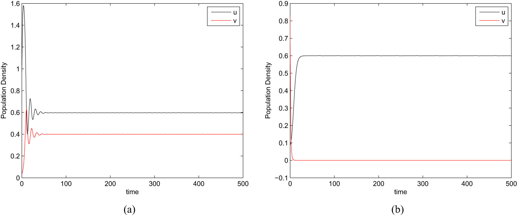
Bifurcation diagram of model system (1) with respect to (a) m and (b) a . All the other parametric values are the same as in equation (5).

In Figure 5, one can observe that higher value of harvesting effort leads to the extinction of zooplankton. At e = 0.06 , both the species show stable dynamics with coexistence, but when we increase e = 3.0 , there is no change in the dynamics however there is an extinction of zooplankton species (Figure 5(b)). We have plotted the bifurcation diagram in Figure 4 taking prey refuge and growth rate of phytoplankton as bifurcation parameters. The bifurcation diagrams of model system (1) at bifurcation parameters m and a provides a more comprehensive understanding of the system’s dynamics (Figures 4(a) and (b)). In Figure 4(a), we observe that, as the prey refuge size is gradually increased, the system experiences Hopf bifurcation resulting in the interior equilibrium point to become stable. Figure 4(b) shows that when the growth rate of phytoplankton is increased, the system undergoes Hopf bifurcation, and the interior equilibrium point becomes unstable.

Figure 5

Time series plot of model system (1) at different values of parameter e . All the parameter values are the same as in equation (5) except (a) e = 0.06 and (b) e = 3.0 .

5 Summary and conclusion

The hiding behavior of prey is crucial in ensuring the survival of species. Seeking refuge allows prey to shield themselves from predators, thus avoiding excessive predation. This contributes to the overall stability of the ecosystem. Additionally, implementing an optimal harvesting policy is essential in preventing the overexploitation of species. The study of Tripathi et al. [28] revealed that harvesting effort acts as a mechanism of biological control for plankton species. In this article, we have proposed a nonlinear mathematical model among phytoplankton and zooplankton species with the combined effects of prey refuge and harvesting. The phytoplankton and zooplankton populations are harvested according to catch per unit effort hypothesis. We have analyzed the linear stability of the model system analytically. We have also derived conditions for bionomic equilibrium and optimal harvesting policy using Pontryagin’s maximum principle. It has been observed that zero discount rate gives the maximum value of the net revenue, while an infinite discount rate leads to zero economic revenue. Numerically, we investigated the dynamics of the plankton model by varying the parameters. We have found that prey refuge and growth rate of phytoplankton have a great impact on the dynamics of the system. The higher value of prey refuge leads to the stable dynamics, whereas the lower value of growth rate of phytoplankton is responsible for the stable behavior of the model system. We can also observe the same behavior from the bifurcation diagram of the model system (Figure 4). In [24], Tripathi and Singh observed that the occurrence of Hopf bifurcation guarantees the survival prospects of all species. Also, we have found the extinction scenario of zooplankton at a higher value of harvesting effort which indicates the bad health of biodiversity of aquatic ecosystem. Thus, management of harvesting effort is much needed for the coexistence of both species.

Acknowledgement

The authors are grateful for the reviewer’s valuable comments that improved the manuscript.

Funding information: This research work of Satish Kumar Tiwari is supported by RGIPT, Jais Amethi (P-2207). The research work of Jai Prakash Tripathi is supported by the Science and Engineering Research Board (SERB), India [File No. MTR/2022/001028].
Author contributions: All authors have accepted responsibility for the entire content of this manuscript and consented to its submission to the journal, reviewed all the results, and approved the final version of the manuscript. Poulomi Basak and Satish Kumar Tiwari proposed the problem, developed the model, and carried out mathematical and numerical analysis. Jai Prakash Tripathi supervised, reviewed, and corrected the manuscript. Vandana Tiwari and Ratnesh Kumar Mishra reviewed the manuscript.
Conflict of interest: There is no conflict of interest to declare.
Ethical statement: This research did not require ethical approval.

References

[1] Agmour, I., Baba, N., Bentounsi, M., Achtaich, N., El Foutayeni, Y. (2021). Mathematical study and optimal control of bioeconomic model concerning harmful dinoflagellate phytoplankton. Computational and Applied Mathematics, 40, 1–16. 10.1007/s40314-021-01509-3Search in Google Scholar

[2] Agnihotri, K., Kaur, H. (2021). Optimal control of harvesting effort in a phytoplankton-zooplankton model with infected zooplankton under the influence of toxicity. Mathematics and Computers in Simulation, 190, 946–964. 10.1016/j.matcom.2021.06.022Search in Google Scholar

[3] Bhattacharjee, R., Gupta, A., Das, N., Agnihotri, A. K., Ohri, A., Gaur, S. (2022). Analysis of algal bloom intensification in mid-ganga river, India, using satellite data and neural network techniques. Environmental Monitoring and Assessment, 194(8), 547. 10.1007/s10661-022-10213-6Search in Google Scholar PubMed PubMed Central

[4] Birkhoff, G., Rota, G. (1982). Ordinary Differential Equation, ginn and co. Boston.Search in Google Scholar

[5] Braselton, J., Braselton, L. (2004). A model of harmful algal blooms. Mathematical and computer modelling, 40(9–10), 923–934. 10.1016/j.mcm.2004.09.001Search in Google Scholar

[6] Chakraborty, S., Bhattacharya, S., Feudel, U., Chattopadhyay, J. (2012). The role of avoidance by zooplankton for survival and dominance of toxic phytoplankton. Ecological complexity, 11, 144–153. 10.1016/j.ecocom.2012.05.006Search in Google Scholar

[7] Chakraborty, S., Chattopadhyay, J. (2008). Nutrient-phytoplankton-zooplankton dynamics in the presence of additional food source – mathematical study. Journal of Biological Systems, 16(04), 547–564. 10.1142/S0218339008002654Search in Google Scholar

[8] Chattopadhayay, J., Sarkar, R. R., Mandal, S. (2002). Toxin-producing plankton may act as a biological control for planktonic blooms – field study and mathematical modelling. Journal of Theoretical Biology, 215(3), 333–344. 10.1006/jtbi.2001.2510Search in Google Scholar PubMed

[9] Chattopadhyay, J., Sarkar, R. R., El Abdllaoui, A. (2002). A delay differential equation model on harmful algal blooms in the presence of toxic substances. Mathematical Medicine and Biology: A Journal of the IMA, 19(2), 137–161. 10.1093/imammb19.2.137Search in Google Scholar

[10] Holling, C. S. (1965). The functional response of predators to prey density and its role in mimicry and population regulation. The Memoirs of the Entomological Society of Canada, 97(S45), 5–60. 10.4039/entm9745fvSearch in Google Scholar

[11] Huang, Y., Chen, F., Zhong, L. (2006). Stability analysis of a prey-predator model with holling type iii response function incorporating a prey refuge. Applied Mathematics and Computation, 182(1), 672–683. 10.1016/j.amc.2006.04.030Search in Google Scholar

[12] Huda, M. N., A’yun, Q. Q., Wigantono, S., Sandariria, H., Raming, I., Asmaidi, A. (2023). Effects of harvesting and planktivorous fish on bioeconomic phytoplankton-zooplankton models with ratio-dependent response functions and time delays. Chaos, Solitons & Fractals, 173, 113736. 10.1016/j.chaos.2023.113736Search in Google Scholar

[13] Ji, J., Lei, C., Yuan, Y. (2023). Qualitative analysis on a reaction-diffusion nutrient-phytoplankton model with toxic effect of holling-type ii functional. Discrete & Continuous Dynamical Systems-Series B, 28(4), 2745–2767. 10.3934/dcdsb.2022190Search in Google Scholar

[14] Li, J., Song, Y., Wan, H., Zhu, H. (2016). Dynamical analysis of a toxin-producing phytoplankton-zooplankton model with refuge. Mathematical Biosciences & Engineering, 14(2), 529–557. Search in Google Scholar

[15] Lv, Y., Pei, Y., Gao, S., Li, C. (2010). Harvesting of a phytoplankton-zooplankton model. Nonlinear Analysis: Real World Applications, 11(5), 3608–3619. 10.1016/j.nonrwa.2010.01.007Search in Google Scholar

[16] Meng, X., Li, J. (2020). Stability and hopf bifurcation analysis of a delayed phytoplankton-zooplankton model with allee effect and linear harvesting. Mathematical Biosciences and Engineering, 17(3), 1973–2002. 10.3934/mbe.2020105Search in Google Scholar PubMed

[17] Pandey, S., Ghosh, U., Das, D., Chakraborty, S., Sarkar, A. (2024). Rich dynamics of a delay-induced stage-structure prey-predator model with cooperative behavior in both species and the impact of prey refuge. Mathematics and Computers in Simulation, 216, 49–76. 10.1016/j.matcom.2023.09.002Search in Google Scholar

[18] Panja, P., Mondal, S. K., Jana, D. K. (2017). Effects of toxicants on phytoplankton-zooplankton-fish dynamics and harvesting. Chaos, Solitons & Fractals, 104, 389–399. 10.1016/j.chaos.2017.08.036Search in Google Scholar

[19] Pontryagin, L. S. (2018). Mathematical theory of optimal processes. London: Routledge. 10.1201/9780203749319Search in Google Scholar

[20] Roy, S., Alam, S., Chattopadhyay, J. (2006). Competing effects of toxin-producing phytoplankton on overall plankton populations in the Bay of Bengal. Bulletin of Mathematical Biology, 68, 2303–2320. 10.1007/s11538-006-9109-5Search in Google Scholar PubMed

[21] Roy, S., Chattopadhyay, J. (2007). Toxin-allelopathy among phytoplankton species prevents competitive exclusion. Journal of Biological Systems, 15(01), 73–93. 10.1142/S021833900700209XSearch in Google Scholar

[22] Sarkar, R. R., Pal, S., Chattopadhyay, J. (2005). Role of two toxin-producing plankton and their effect on phytoplankton-zooplankton system-a mathematical study supported by experimental findings. BioSystems, 80(1), 11–23. 10.1016/j.biosystems.2004.09.029Search in Google Scholar PubMed

[23] Shaika, N., Khan, S., Sultana, S. (2022). Harmful algal blooms in the coastal waters of Bangladesh: an overview. Journal of Aquaculture & Marine Biology, 11(3), 105–111. 10.15406/jamb.2022.11.00344Search in Google Scholar

[24] Tripathi, D., Singh, A. (2023). An eco-epidemiological model with predator switching behavior. Computational and Mathematical Biophysics, 11(1), 20230101. 10.1515/cmb-2023-0101Search in Google Scholar

[25] Tripathi, J. P., Abbas, S., Thakur, M. (2015). A density dependent delayed predator-prey model with Beddington-Deangelis type function response incorporating a prey refuge. Communications in Nonlinear Science and Numerical Simulation, 22, 427–450. 10.1016/j.cnsns.2014.08.018Search in Google Scholar

[26] Tripathi, J. P., Abbas, S., Thakur, M. (2015). Dynamical analysis of a prey-predator model with beddington-deangelis type function response incorporating a prey refuge. Nonlinear Dynamics, 80, 177–196. 10.1007/s11071-014-1859-2Search in Google Scholar

[27] Tripathi, J. P., Jana, D. D., Vyshnavi Devi, N., Tiwari, V., Abbas, S. (2020). Intraspecific competition of predator for prey with variable rates in protected areas. Nonlinear Dynamics, 102, 511–535. 10.1007/s11071-020-05951-6Search in Google Scholar

[28] Tripathi, J. P., Tripathi, D., Mandal, S., Shrimali, M. (2023). Cannibalistic enemy-pest model: effect of additional food and harvesting. Journal of Mathematical Biology, 87, 58. 10.1007/s00285-023-01991-9Search in Google Scholar PubMed

[29] Xiang, H., Liu, B., Fang, Z. (2018). Optimal control strategies for a new ecosystem governed by reaction-diffusion equations. Journal of Mathematical Analysis and Applications, 467(1), 270–291. 10.1016/j.jmaa.2018.07.001Search in Google Scholar

[30] Zhang, H., Niu, B. (2020). Dynamics in a plankton model with toxic substances and phytoplankton harvesting. International Journal of Bifurcation and Chaos, 30(2), 2050035. 10.1142/S0218127420500352Search in Google Scholar

Received: 2024-03-23

Revised: 2024-07-25

Accepted: 2024-08-12

Published Online: 2024-09-30

This work is licensed under the Creative Commons Attribution 4.0 International License.

Articles in the same Issue

https://doi.org/10.1515/cmb-2024-0011

Keywords for this article

optimal harvesting policy; stability analysis; harmful algal blooms; prey refuge; bionomic equilibrium

Creative Commons

BY 4.0