Analysis and numerical simulation of fractional-order blood alcohol model with singular and non-singular kernels

Amit Prakash; Neha Kalyan; Sanjeev Ahuja

doi:10.1515/cmb-2024-0001

Article Open Access

Analysis and numerical simulation of fractional-order blood alcohol model with singular and non-singular kernels

Amit Prakash , Neha Kalyan and Sanjeev Ahuja

Published/Copyright: April 8, 2024

Published by

Become an author with De Gruyter Brill

Submit Manuscript Author Information

From the journal Computational and Mathematical Biophysics Volume 12 Issue 1

Abstract

In this manuscript, we examine the blood alcohol model to investigate the dynamics of alcohol concentration in the human body. The classical model of blood alcohol concentration is converted into the fractional model by using Caputo, Caputo-Fabrizio (CF), and Atangana-Baleanu-Caputo derivatives. The existence and uniqueness theory for the model’s solution is constructed using the Banach fixed point theory. Also, the stability of the solution is established by Ulam-Hyers conditions. For the numerical simulation of the considered model, the Adams-Bashforth method with a two-step Lagrange polynomial is used and the numerical solution of the model with three different derivatives is presented in the tabular and graphical form. The comparison between the exact solution and observed solution is made by root mean square technique which is found to be in good agreement. Finally, the results from the three fractional derivatives are also compared with the exact data, which revealed that the CF fractional derivative performs better than the other two fractional derivatives.

Keywords: blood alcohol model; Caputo fractional derivative; Caputo-Fabrizio fractional derivative; Atangana-Baleanu-Caputo derivatives; fixed point theorem; Ulam-Hyers stability; Adams-Bashforth method

MSC 2010: 26A33; 65L99; 34A08

1 Introduction

Fractional calculus is an area of applied mathematics concerned with fractional-order derivatives and integrals. Real-world situations involving fractional calculus can capture the physical description of the concept better than classical calculus. Due to numerous important applications in science and engineering, non-integer-order (fractional) derivatives have caught the interest of many scientists. Fractional differential equations [22,27] have been used to model a variety of engineering and physical phenomena. The fractional-order models have received a lot of attention recently since they are more accurate and realistic than classical-order models. The classical- or integer-order derivatives are local in nature, i.e., it does not capture the model’s entire memory, whereas non-integer derivatives carry their present as well as past information [35]. Several researchers have utilized these fractional derivatives to solve various problems with different techniques such as homotopy analysis transform technique (HATM) [36,37], conformable fractional differential transform method [43], q-homotopy analysis transform method [28,30], iterative method [38,39], and fractional variational iteration method [20], homotopy perturbation transform method [18].

Alcohol is a poisonous and intoxicating substance that can cause addiction. In today’s societies, many people use alcoholic beverages on a regular basis. The liver uses enzymes to metabolize alcohol. In contrast, the liver can process a little amount of alcohol at one time, enabling the excess to spread all over the body. Alcohol has an effect on all of the body’s organs. The effect of alcohol on the human body depends on the amount consumed. According to the World Health Organization [25], worldwide, 3 million people die every year from unhealthy alcohol usage, accounting for 5.3% of all deaths. Harmful alcohol usage has been connected to more than 200 diseases and injuries. Alcohol is responsible for 13.5% of all deaths in the 20- to 39-year-old age group. At first, Ludwin [24] solves a set of differential equations that describe blood alcohol concentration as a function of time given as

(1) d S d t = − k 1 S ( t ) , d B d t = k 1 S ( t ) − k 2 B ( t ) .

The exact solution for the classical blood alcohol model by direct integration of the system of equation (1) is given in Table 1.

Table 1

Exact data for blood alcohol levels [24]

Time (min)	Blood alcohol level (mg/L)
0	0
10	147.54
20	172.95
30	161.38
45	129.99
80	70.99
90	59.49
110	41.74
170	14.41

Now, we generalize the integer-order differential equations of the considered model into the fractional differential equations as the fractional model more appropriately represents the system because of its additional remembrance and inheritance qualities, which make it particularly effective in replicating and analyzing real occurrences. This is primarily due to two factors: (a) it is possible to choose any arbitrary order of fractional operators, whereas this is not possible with standard order derivatives, and (b) because classical-order derivatives are local in nature, they do not describe the entire memory and physical aspects of the model, whereas fractional-order derivatives are non-local in nature and thus describe the entire memory and physical behavior of the system. So, we convert the blood alcohol model into the fractional version by using three fractional operators:

Caputo differential operator:
(2) D t α 0 C S ( t ) = − k 1 S ( t ) , D t α 0 C B ( t ) = k 1 S ( t ) − k 2 B ( t ) .
Caputo-Fabrizio (CF) differential operator:
(3) D t α 0 CF ( t ) = − k 1 S ( t ) , D t α 0 CF B ( t ) = k 1 S ( t ) − k 2 B ( t ) .
Atangana-Baleanu-Caputo (ABC) differential operator:
(4) D t α 0 ABC S ( t ) = − k 1 S ( t ) , D t α 0 ABC B ( t ) = k 1 S ( t ) − k 2 B ( t ) ,

subject to the initial conditions:

S ( 0 ) = S 0 , B ( 0 ) = B 0 = 0 ,

where S ( t ) represents the alcohol concentration (mg/L) at time t (min) in the stomach, B ( t ) represents the alcohol concentration (mg/L) at time t (min) in the blood, k 1 is the first constant of rate law and k 2 is the second constant of rate law, and S 0 and B 0 represents the initial alcohol concentration in the stomach and blood, respectively.

Because of the serious consequences on human life, alcohol addiction has caught the interest of many scholars and researchers from a wide range of fields: Almeida et al. [4] compared the integer- and fractional-order modeling approaches to some real-world problems including the blood alcohol concentration problem with real data and found that the fractional-order equation more accurately describes the model’s dynamics. Singh [35] studied the blood alcohol model with the Sumudu transform via the Hilfer fractional operator. Qureshi et al. [32] investigated the fractional blood ethanol model with Caputo, CF, and ABC derivatives, and for the solution, the Laplace transform is used. The Caputo and ABC derivative operators outperform the standard order model in estimating real data; however, the CF operator produces the same results as the original integer-order model. Bunonyo and Amadi [13] studied the movement of alcohol in the gastrointestinal tract and bloodstream, as well as its impact on the human body.

In this article, we solve a set of differential equations of the blood alcohol model. To calculate an approximate fractional solution of the considered problem, the two-step Adams-Bashforth numerical method with Lagrange polynomial is used. Several researchers have successfully used the Adams-Bashforth method (ABM) to solve fractional differential equations such as the time fractional Tricomi equation [21], stem cell differentiation [40], the tumor dynamics model [5], the predator-prey problem [26], and Influenza A epidemic model [17]. Several fractional derivatives including Riemann-Liouville, Caputo, Riesz, Grunwald-Letnikov, CF, and ABC have been developed in the literature. In this work, we utilize Caputo, CF, and ABC to solve the proposed problem. The Caputo fractional derivative uses a power law kernel, which is singular whereas CF and ABC fractional derivatives use the exponential kernel and the Mittag-Leffler kernel, respectively, which are non-singular kernels. These fractional derivatives have been used by many researchers for solving linear and non-linear problems [3,6,7,9–12,14,19,23,29,31,34,42]. Also, the existence and uniqueness for the solution are done by fixed point theory, and Ulam-Hyers (UH) stability is discussed, which is widely investigated by numerous researchers [16,41,46,47].

This article is organized in various sections as follows: in Section 1, we present the introduction and description of the model used in this study. In Section 2, important definitions that are used in this article are given. Section 3 includes the existence and uniqueness conditions for the solution of the problem. In Section 4, stability conditions are constructed for the solution of the considered model. In Section 5, the numerical algorithm for the solution of the blood alcohol model is constructed using the two-step ABM. In Section 6, numerical simulation, a graphical representation of the solution of the fractional blood alcohol model via MATLAB-21 software, and a comparison between the experimental data and data obtained by this study are presented. Finally, Section 7 contains the conclusion.

2 Mathematical preliminaries

The fractional derivatives and integrals of Caputo, CF, and ABC are provided in this section as follows:

Definition 2.1

The fractional-order derivative of the function f ( t ) in the Caputo sense with order α > 0 , where m − 1 ≤ α ≤ m , m ∈ N , is given as [27]

D t α 0 C [ f ( t ) ] = 1 Γ ( m − α ) ∫ 0 t ( t − τ ) m − α − 1 f m ( τ ) d τ .

Definition 2.2

The fractional integration of the function f ( t ) in the Caputo sense with order α > 0 , where m − 1 ≤ α ≤ m , m ∈ N , is given as [27]

I t α 0 C [ f ( t ) ] = 1 Γ ( α ) ∫ 0 t ( t − τ ) α − 1 f ( τ ) d τ .

Definition 2.3

The CF derivative of the function f ( t ) of order α > 0 is defined as [15]

D t α 0 CF f ( t ) = M ( α ) 1 − α ∫ 0 t e − α 1 − α ( t − τ ) d d τ [ f ( τ ) ] d τ ,

where M ( α ) is the normalization function that satisfies M ( 0 ) = M ( 1 ) = 1 , f ∈ H 1 ( 0 , 1 ) , and α ∈ ( 0 , 1 ] .

Definition 2.4

Integration of a function f ( t ) in CF sense of order α > 0 is defined as [15]

I t α 0 CF f ( t ) = 1 − α M ( α ) f ( τ ) + α M ( α ) ∫ 0 t f ( τ ) d τ .

Definition 2.5

The fractional-order derivative of f ( t ) in ABC sense with order α > 0 is given by [8]

D t α 0 ABC f ( t ) = ABC ( α ) 1 − α ∫ 0 t E α − α 1 − α ( t − τ ) α d d τ [ f ( τ ) ] d τ ,

where ABC ( α ) = α 2 − α is the normalization function, and E α is the “Mittag-Leffler function” given as

E α ( y ) = ∑ k = 0 ∞ y k Γ ( α k + 1 ) .

Definition 2.6

The fractional integration of the function f ( t ) in the ABC sense with order α > 0 is given by [8]

I t α 0 ABC f ( t ) = 1 − α ABC ( α ) f ( t ) + α ABC ( α ) Γ ( α ) ∫ 0 t ( t − τ ) α − 1 f ( τ ) d τ .

3 Existence and uniqueness of solution

In this section, we prove the existence and uniqueness for the solution of the considered model with three fractional derivatives. For this purpose, we first take system (2) of differential equations with Caputo fractional operator, and for the existence of the solution, we define a Banach space ξ = ψ × ψ , where ψ = C ( ζ ) under the norm ‖ U ‖ = max t ∈ ζ [ ∣ S ( t ) ∣ + ∣ B ( t ) ∣ ] = ‖ ( S , B ) ‖ , where ζ = [ 0 , T ] , and U = ( S , B ) ∈ ξ .

Let us express the right-hand side of the proposed model as

(5) f 1 ( t , S , B ) = − k 1 S ( t ) , f 2 ( t , S , B ) = k 1 S ( t ) − k 2 B ( t ) .

So, Problem (2) can be written as

(6) D t α 0 C S ( t ) = f 1 ( t , S , B ) , D t α 0 C B ( t ) = f 2 ( t , S , B ) .

We can write this equation in the vector form as

(7) D t α 0 C U ( t ) = F ( t , U ( t ) ) , 0 < α ≤ 1 ,

U ( 0 ) = U 0 ,

where

(8) U ( t ) = S ( t ) B ( t ) , U 0 = S 0 B 0 , F ( t , U ( t ) ) = f 1 ( t , S , B ) f 2 ( t , S , B ) .

By integrating both sides of the (7), we obtain

(9) U ( t ) = U 0 + 1 Γ ( α ) ∫ 0 t F ( τ , U ( τ ) ) ( t − τ ) α − 1 d τ .

Let J : ξ → ξ be an operator, which is defined by

(10) J ( U ) ( t ) = U 0 + 1 Γ ( α ) ∫ 0 t F ( τ , U ( τ ) ) ( t − τ ) α − 1 d τ .

We use the following theorems and hypotheses to prove the existence and uniqueness of the solution of Model (2):

Theorem 3.1

[2] Let J : ξ → ξ be a completely continuous operator, and let

D ( J ) = { U ∈ ξ : U = λ J ( U ) , λ ∈ [ 0 , 1 ] }

be bounded. Then, there exists at least one fixed point of J in ξ .

Hypothesis (A). There exists a constant L > 0 such that for U , U ¯ ∈ ξ , we have

∣ F ( t , U ( t ) ) − F ( t , U ¯ ( t ) ) ∣ ≤ L ∣ U ( t ) − U ( t ) ¯ ∣ .

For simplicity, we use the following notation:

Δ = T α Γ ( α + 1 ) .

Proof

To prove that the operator J is completely continuous. Let us take a sequence { U n } such that U n → U in ξ , then for any t ∈ ζ , we have

∥ J ( U n ) − J ( U ) ∥ ≤ 1 Γ ( α ) max t ∈ ζ ∫ 0 t ∣ F ( τ , U n ( τ ) ) − F ( τ , U ( τ ) ) ∣ ( t − τ ) α − 1 d τ , ≤ L Γ ( α ) ∥ U n − U ∥ max t ∈ ζ ∫ 0 1 t α ( 1 − z ) α − 1 d z , ≤ L T α Γ ( α ) ∥ U n − U ∥ max t ∈ ζ ∫ 0 1 ( 1 − z ) α − 1 d z , ≤ L T α α Γ ( α ) ∥ U n − U ∥ , ≤ L T α Γ ( α + 1 ) ∥ U n − U ∥ , ≤ L Δ ∥ U n − U ∥ .

Since sequence U n → U , ∥ J ( U n ) − J ( U ) ∥ → 0 as n → 0 . Thus, the operator J is continuous.

Suppose S ⊂ ξ is a bounded set. Then, ∣ F ( t , U ( t ) ) ∣ ≤ C , C > 0 , ∀ U ∈ S .

Then, for each U ∈ S , we obtain

∥ J ( U ) ∥ ≤ C Γ ( α ) max t ∈ ζ ∫ 0 t ( t − τ ) α − 1 d τ , ≤ C T α α Γ ( α ) , ≤ C Δ .

Hence, the operator J is uniformly bounded.

Now, take 0 ≤ t 2 ≤ t 1 ≤ T , then

∥ J ( U ) ( t 1 ) − J ( U ) ( t 2 ) ∥ ≤ C Γ ( α ) max t ∈ ζ ∫ 0 t 1 ( t 1 − τ ) α − 1 d τ − ∫ 0 t 2 ( t 2 − τ ) α − 1 d τ , ≤ C Γ ( α ) max t ∈ ζ ∫ 0 t 1 ( t 1 − τ ) α − 1 d τ − ∫ 0 t 2 ( t 2 − τ ) α − 1 d τ , ≤ C α Γ ( α ) ( t 1 α − t 2 α ) → 0 , as t 1 → t 2 .

Hence, J is equicontinuous. Also, J is bounded and continuous, so relatively compact, and thus, J is completely continuous.

Now, we prove that D is a bounded set.

Let us take U ∈ D , then for any t ∈ ζ , we have

∥ U ( t ) ∥ = ∥ λ J ( U ( t ) ) ∥ ≤ λ C Δ .

Therefore, D is bounded. Hence, with the use of Theorem 3.1, Model (2) has at least one solution.□

Theorem 3.2

[2] Problem (2) has a unique solution if we assume hypothesis (A) and Θ < 1 , where

Θ = Δ L .

Proof

For U , U ¯ ∈ ξ and each t ∈ ζ , we can obtain

(11) ∥ J ( U ) − J ( U ¯ ) ∥ ≤ 1 Γ ( α ) max t ∈ ζ ∫ 0 t F ( τ , U ( τ ) ) ( t − τ ) α − 1 d τ − ∫ 0 t F ( τ , U ¯ ( τ ) ) ( t − τ ) α − 1 d τ , ≤ Δ L ∥ U − U ¯ ∥ , ≤ Θ ∥ U − U ¯ ∥ .

Hence, J has a contraction. This shows that Problem (2) has a unique solution.□

Using a similar technique, we can prove the existence and uniqueness of the solution for the blood alcohol model with CF and ABC fractional operators [44,45].

4 Stability analysis

In this section, we prove the stability for the solution of the system of differential equations (2) using UH stability analysis technique.

For UH-stability, take a small perturbation Q ∈ C ( ζ ) ; Q ( 0 ) = 0 , and

∣ Q ( t ) ∣ ≤ ε , for ε > 0 ,
D t α 0 C U ( t ) = F ( t , U ( t ) ) + Q ( t ) .

Lemma 4.1

The solution for the following problem:

(12) D t α 0 C U ( t ) = F ( t , U ( t ) ) + Q ( t ) , U ( 0 ) = U 0 ,

satisfies the relation given as

(13) U ( t ) − U 0 + 1 Γ ( α ) ∫ 0 t F ( τ , U ( τ ) ) ( t − τ ) α − 1 d τ ≤ Δ ε .

Proof

Using equation (9), we obtain the solution for Problem (12) as:

(14) U ( t ) = U 0 + 1 Γ ( α ) ∫ 0 t ( F ( τ , U ( τ ) ) + Q ( τ ) ) ( t − τ ) α − 1 d τ .

Using the relation ∣ Q ( t ) ∣ ≤ ε in equation (14), we can easily obtain Relation (13).□

Theorem 4.1

[1] Let us suppose the hypothesis (A) and Relation (11) hold. Also, Θ < 1 , where Θ = Δ L . Then, the solution of Problem (2) is UH stable.

Proof

Let W be a unique solution of equation (9) and U be any solution of equation (9), then

∥ U ( t ) − W ( t ) ∥ = U ( t ) − W 0 + 1 Γ ( α ) ∫ 0 t F ( τ , W ( τ ) ) ( t − τ ) α − 1 d τ , ≤ U ( t ) − U 0 + 1 Γ ( α ) ∫ 0 t F ( τ , U ( τ ) ) ( t − τ ) α − 1 d τ + U 0 + 1 Γ ( α ) ∫ 0 t F ( τ , U ( τ ) ) ( t − τ ) α − 1 d τ − W 0 + 1 Γ ( α ) ∫ 0 t F ( τ , W ( τ ) ) ( t − τ ) α − 1 d τ .

Using equations (11) and (13), we obtain

∥ U ( t ) − W ( t ) ∥ ≤ Δ ε + Θ ∥ U − W ∥ .

Therefore, we can write

(15) ∥ U − W ∥ ≤ P ,

where P = Δ ε 1 − Θ . Thus, from (15), we conclude that Problem (2) is UH stable.□

Similarly, we can prove the stability of the blood alcohol model with CF and ABC fractional operators [33,47].

5 Numerical algorithm

In this section, the numerical algorithm for the solution of the blood alcohol model with three different fractional derivatives is constructed using the fractional two-step ABM.

5.1 Numerical solution of blood alcohol model in the sense of Caputo fractional derivative

Now, we evaluate the numerical solution of Model (2). For this, let us take the first equation of System (2) with the initial condition as

(16) D t α 0 C S ( t ) = f 1 ( t , S , B ) , S ( 0 ) = S 0 .

By integration, the solution of equation (16) is given by

(17) S ( t ) = S 0 + 1 Γ ( α ) ∫ 0 t f 1 ( τ , S , B ) ( t − τ ) α − 1 d τ .

Now, we develop the numerical algorithm for the considered system using t i + 1 in place of t in equation (17), we obtain

S i + 1 = S 0 + 1 Γ ( α ) ∫ 0 t i + 1 f 1 ( τ , S , B ) ( t i + 1 − τ ) α − 1 d τ .

Then, by approximating the above obtained integral, we obtain

(18) S i + 1 = S 0 + 1 Γ ( α ) ∑ m = 0 i ∫ t m t m + 1 f 1 ( τ , S , B ) ( t i + 1 − τ ) α − 1 d τ .

Now, using the two-step Lagrange polynomial, one can write over [ t m , t m + 1 ] the function f 1 ( τ , S , B ) with h = t m − t m + 1 such that

(19) f 1 ( τ , S , B ) = 1 h [ ( τ − t m − 1 ) f 1 ( t m , S , B ) − ( τ − t m ) f 1 ( t m − 1 , S , B ) ] .

By substituting equation (19) into equation (18), we have

(20) S i + 1 = S 0 + 1 Γ ( α ) ∑ m = 1 i ∫ t m t m + 1 1 h [ ( τ − t m − 1 ) f 1 ( t m , S , B ) ( t i + 1 − τ ) α − 1 ] − [ ( τ − t m ) f 1 ( t m − 1 , S , B ) ] ( t i + 1 − τ ) α − 1 d τ .

After evaluating the integral of (20), we obtain the numerical solution for the first equation of the system (2) as:

(21) S i + 1 = S 0 + h α Γ ( α + 2 ) ∑ m = 1 i [ f 1 ( t m , S , B ) ( ( i + 1 − m ) α ( i − m + 2 + α ) − ( i − m ) α ( i − m + 2 + 2 α ) ) − f 1 ( t m − 1 , S , B ) ( ( i + 1 − m ) α + 1 − ( i − m ) α ( i − m + 1 + α ) ) ] .

Similarly, we can obtain the numerical solution of the second equation of System (2) as

(22) B i + 1 = B 0 + h α Γ ( α + 2 ) ∑ m = 1 i [ f 2 ( t m , S , B ) ( ( i + 1 − m ) α ( i − m + 2 + α ) − ( i − m ) α ( i − m + 2 + 2 α ) ) − f 2 ( t m − 1 , S , B ) ( ( i + 1 − m ) α + 1 − ( i − m ) α ( i − m + 1 + α ) ) ] .

5.2 Numerical solution of blood alcohol model in the sense of CF fractional derivative

Now, to solve System (3), we take the first equation of System (3) with the initial condition as

(23) D t α 0 CF ( t ) = f 1 ( t , S , B ) , S ( 0 ) = S 0 .

By integrating in the CF sense, we obtain

(24) S ( t ) = S 0 + 1 − α M ( α ) f 1 ( t , S , B ) + α M ( α ) ∫ 0 t f 1 ( τ , S , B ) d τ .

Now, we develop the numerical algorithm for the considered system using t i + 1 in place of t in equation (24), and we obtain

S i + 1 = S 0 + 1 − α M ( α ) f 1 ( t i , S , B ) + α M ( α ) ∫ 0 t i + 1 f 1 ( τ , S , B ) d τ .

Then, by approximating the above obtained integral, we obtain

(25) S i + 1 = S 0 + 1 − α M ( α ) f 1 ( t i , S , B ) + α M ( α ) ∑ m = 0 i ∫ t m t m + 1 f 1 ( τ , S , B ) d τ .

Now, using the two-step Lagrange polynomial for the function f 1 ( τ , S , B ) in the aforementioned equation, we obtain

(26) S i + 1 = S 0 + 1 − α M ( α ) f 1 ( t i , S , B ) + α M ( α ) ∑ m = 1 i ∫ t m t m + 1 1 h [ ( τ − t m − 1 ) f 1 ( t m , S , B ) − ( τ − t m ) f 1 ( t m − 1 , S , B ) ] d τ .

After evaluating the integral of (26), we obtain the numerical solution for the first equation of System (3) as

(27) S i + 1 = S 0 + 1 − α M ( α ) f 1 ( t i , S , B ) + α h 2 M ( α ) ∑ m = 1 i [ 3 f 1 ( t m , S , B ) − f 1 ( t m − 1 , S , B ) ] .

Similarly, we can obtain the numerical solution of the second equation of System (3) as

(28) B i + 1 = B 0 + 1 − α M ( α ) f 2 ( t i , S , B ) + α h 2 M ( α ) ∑ m = 1 i [ 3 f 2 ( t m , S , B ) − f 2 ( t m − 1 , S , B ) ] .

5.3 Numerical solution of blood alcohol model in the sense of ABC fractional derivative

Now, to find the solution for System (4), we take the first equation of the system with the initial condition as

(29) D t α 0 ABC S ( t ) = f 1 ( t , S , B ) , S ( 0 ) = S 0 .

By integrating in the Atangana-Baleanu sense, we obtain

(30) S ( t ) = S 0 + 1 − α A B C ( α ) f 1 ( t , S , B ) + α A B C ( α ) Γ ( α ) ∫ 0 t f 1 ( τ , S , B ) ( t − τ ) α − 1 d τ .

Now, we develop the numerical algorithm for the considered system using t i + 1 in place of t in equation (30), we obtain

S i + 1 = S 0 + 1 − α A B C ( α ) f 1 ( t i , S , B ) + α A B C ( α ) Γ ( α ) ∫ 0 t i + 1 f 1 ( τ , S , B ) ( t i + 1 − τ ) α − 1 d τ .

Then, by approximating the above obtained integral, we obtain

(31) S i + 1 = S 0 + 1 − α A B C ( α ) f 1 ( t i , S , B ) + α A B C ( α ) Γ ( α ) ∑ m = 0 i ∫ t m t m + 1 f 1 ( τ , S , B ) ( t i + 1 − τ ) α − 1 d τ .

Now, using the two-step Lagrange polynomial for the function f 1 ( τ , S , B ) in the aforementioned equation, we obtain

(32) S i + 1 = S 0 + 1 − α A B C ( α ) f 1 ( t i , S , B ) + α A B C ( α ) Γ ( α ) × ∑ m = 1 i ∫ t m t m + 1 1 h [ ( τ − t m − 1 ) f 1 ( t m , S , B ) − ( τ − t m ) f 1 ( t m − 1 , S , B ) ] ( t i + 1 − τ ) α − 1 d τ .

After evaluating the integral of (32), we obtain the numerical solution for the first equation of System (4) as:

(33) S i + 1 = S 0 + 1 − α ABC ( α ) f 1 ( t i , S , B ) + α h α ABC ( α ) Γ ( α + 2 ) × ∑ m = 1 i [ f 1 ( t m , S , B ) ( ( i + 1 − m ) α ( i − m + 2 + α ) − ( i − m ) α ( i − m + 2 + 2 α ) ) − f 1 ( t m − 1 , S , B ) ( ( i + 1 − m ) α + 1 − ( i − m ) α ( i − m + 1 + α ) ) ] .

Similarly, we obtain the numerical solution of the second equation of System (4) as:

(34) B i + 1 = B 0 + 1 − α A B C ( α ) f 2 ( t i , S , B ) + α h α A B C ( α ) Γ ( α + 2 ) × ∑ m = 1 i [ f 2 ( t m , S , B ) ( ( i + 1 − m ) α ( i − m + 2 + α ) − ( i − m ) α ( i − m + 2 + 2 α ) ) − f 2 ( t m − 1 , S , B ) ( ( i + 1 − m ) α + 1 − ( i − m ) α ( i − m + 1 + α ) ) ] .

6 Numerical simulation and discussion

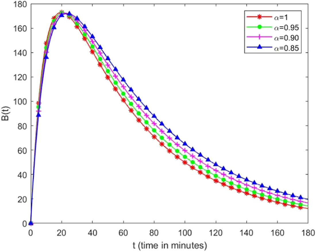
In this section, we present numerical simulations for the fractional derivatives with singular and non-singular kernels to demonstrate the adaptability and effectiveness of the suggested approach. We find the numerical solution of the concentrations of S ( t ) and B ( t ) at various orders of derivative values α with the two-step Adams-Bashforth approach. We have simulated the outcomes corresponding to the initial values and parameters values given in [24] as: S 0 = 245.8769 , B 0 = 0 , k 1 = 0.109456 , and k 2 = 0.017727 . We derive the numerical solution of Models (2), (3), and (4) with a step size of 0.01 and compare it with exact data (Table 1) by varying the order of derivative and present graphically.

Figure 1 represents the plots of alcohol concentration in the blood, and Figure 2 represents the plots of alcohol concentration in the stomach at different orders of derivatives with the use of Caputo fractional derivative, and the comparison of the obtained concentration in the blood with the exact data (Table 1) is given in Table 2. Figure 3 represents the plots of alcohol concentration in the blood, and Figure 4 represents the plots of alcohol concentration in the stomach at different orders of derivatives with the use of CF fractional derivative, and the comparison of the obtained concentration in the blood with the exact data is given in Table 3. Figure 5 represents the plots of alcohol concentration in the blood, and Figure 6 represents the plots of alcohol concentration in the stomach at different orders of derivatives with the use of ABC fractional derivative and the comparison of the obtained concentration in the blood with the exact data is given in Table 4. The comparison of the obtained solution with the exact solution at order of derivative 1 is shown in Table 5. Finally, the comparison of the solutions obtained via three different fractional derivatives (Caputo, C-F, and ABC) at order 0.98 with the exact solution is given in Table 6 and graphically in Figure 7.

$Figure 1 Numerical solution of concentration of alcohol in the blood for distinct values of fractional order in Caputo sense.$

Figure 1

Numerical solution of concentration of alcohol in the blood for distinct values of fractional order in Caputo sense.

$Figure 2 Numerical solution of concentration of alcohol in the stomach for distinct values of fractional order in Caputo sense.$

Figure 2

Numerical solution of concentration of alcohol in the stomach for distinct values of fractional order in Caputo sense.

Table 2

Numerical simulation of blood alcohol concentration at different orders of fractional derivative for h = 0.01

Time (min)	Exact solution (mg/L)	ABM via Caputo derivative
		( α = 1 )	( α = 0.95 )	( α = 0.90 )	( α = 0.85 )
0	0	0	0	0	0
10	147.54	147.4738	138.2144	129.2469	120.5841
20	172.95	172.9503	166.9093	159.6504	151.4678
30	161.38	161.3998	163.1713	162.0004	158.3290
45	129.99	130.0232	141.6989	149.3290	153.0784
80	70.99	71.0143	92.3180	110.9856	126.0763
90	59.49	59.5015	81.4995	101.5619	118.5125
110	41.74	41.7492	63.7829	85.2951	104.7590
170	14.41	14.4126	32.0424	52.5126	74.0149

$Figure 3 Numerical solution of alcohol concentration in the blood for distinct values of fractional order in CF sense.$

Figure 3

Numerical solution of alcohol concentration in the blood for distinct values of fractional order in CF sense.

$Figure 4 Numerical solution of alcohol concentration in the stomach for distinct values of fractional order in CF sense.$

Figure 4

Numerical solution of alcohol concentration in the stomach for distinct values of fractional order in CF sense.

Table 3

Numerical simulation of blood alcohol concentration at different orders of fractional derivative for h = 0.01

Time (min)	Exact solution (mg/L)	ABM via CF derivative
		( α = 1 )	( α = 0.95 )	( α = 0.90 )	( α = 0.85 )
0	0	0	0	0	0
10	147.54	147.4738	143.9327	140.1599	136.1480
20	172.95	172.9503	172.4876	171.6417	170.3714
30	161.38	161.3998	163.8521	166.0410	167.9077
45	129.99	130.0232	134.7196	139.4344	144.1239
80	70.99	71.0143	76.2304	81.8065	87.7594
90	59.49	59.5015	64.4616	69.8193	75.6019
110	41.74	41.7492	46.0576	50.8007	56.0202
170	14.41	14.4126	16.7839	19.5401	22.7428

$Figure 5 Numerical solution of alcohol concentration in the blood for distinct values of fractional order in ABC sense.$

Figure 5

Numerical solution of alcohol concentration in the blood for distinct values of fractional order in ABC sense.

$Figure 6 Numerical solution of alcohol concentration in the stomach for distinct values of fractional order in ABC sense.$

Figure 6

Numerical solution of alcohol concentration in the stomach for distinct values of fractional order in ABC sense.

Table 4

Numerical simulation of blood alcohol concentration at different orders of fractional derivative for h = 0.01

Time (min)	Exact solution (mg/L)	ABM via ABC derivative
		( α = 1 )	( α = 0.95 )	( α = 0.90 )	( α = 0.85 )
0	0	0	0	0	0
10	147.54	147.4738	134.7580	122.3870	110.5157
20	172.95	172.9503	165.7525	155.9312	144.2809
30	161.38	161.3998	164.4906	162.3382	155.8272
45	129.99	130.0232	145.3076	154.1171	156.5160
80	70.99	71.0143	97.2955	119.9231	136.8142
90	59.49	59.5015	86.4386	110.8435	130.2508
110	41.74	41.7492	68.4356	94.7477	117.7008
170	14.41	14.4126	35.3526	60.7350	87.3530

Table 5

Comparison of our method solution with the exact solution at order of derivative, α = 1

Time (min)	Exact solution (mg/L)	Our method solution
0	0	0
10	147.54	147.4738
20	172.95	172.9503
30	161.38	161.3998
45	129.99	130.0232
80	70.99	71.0143
90	59.49	59.5015
110	41.74	41.7492
170	14.41	14.4126

Table 6

Comparison of exact blood alcohol content data with data obtained by using three different types of derivatives with h = 0.01 and order of derivative, α = 0.98

Time (min)	Exact solution (mg/L)	Caputo derivative	CF derivative	ABC derivative
0	0	0	0	0
10	147.54	143.7359	146.0847	142.3574
20	172.95	170.7002	172.8087	170.4388
30	161.38	162.4889	162.4089	163.3129
45	129.99	135.1813	131.8972	136.8909
80	70.99	79.7794	73.0587	81.8079
90	59.49	68.4465	61.4396	70.4041
110	41.74	50.5203	43.4230	52.2713
170	14.41	21.0200	15.3185	22.0867

$Figure 7 Comparison of the solutions with exact data at order of derivative α = 0.98 \alpha =0.98 .$

Figure 7

Comparison of the solutions with exact data at order of derivative α = 0.98 .

The comparison between the obtained solution with the proposed method and the exact solution (from [24]) is made by calculating the root mean square error (RMSE) using equation (35) and is found to be 0.027, and the average accuracy of the numerical technique is found to be 99.9%.

(35) RMSE = ∑ i = 1 n ( e i − o i ) 2 n ,

where e i and o i are the exact and observed values, respectively, and n is the number of values obtained. So, from the obtained results, we can say that the technique used is capable for solving such types of problems with great accuracy. Also, it is clear from the obtained results that the values obtained by the CF differential operator give values closer to the exact data as compared to the values obtained by Caputo and ABC operators in the case of fractional order, which is evidenced by Table 6. So, the CF operator gives satisfactory results as compared to Caputo and ABC operators.

7 Conclusion

In this article, we investigated the blood alcohol model using three different fractional derivative operators. First, we utilize the Banach fixed point theorem to construct the existence and uniqueness requirements for the solution of the considered model, and UH stability analysis is performed to show the stability of the method. The solution for the alcohol concentration in the blood and stomach has been discussed by applying the Adams-Bashforth approach. The graphical data for alcohol concentrations in the stomach and blood are given for distinct values of fractional derivatives. The comparison between the proposed technique and the exact solution is made by finding RMSE and found to be in good agreement. Also, the comparison of the solutions via three derivatives with exact data revealed that the CF operator shows better performance than the other two operators. Hence, we can conclude that ABM with the CF fractional derivative works quite well for mathematical modeling of real-world difficulties, as evidenced by the examination of the blood alcohol model.

Acknowledgements

We thank anonymous reviewers for their constructive suggestions that have helped to improve the quality of the article.

Funding information: This research received no specific grant from any funding agency, commercial or non profit sector.
Conflict of interest: The authors declare that there is no conflict of interest in this article.
Ethics statement: This research did not require ethical approval.

References

[1] Ali, A., Rahman, M., Arfan, M., Shah, Z., Kumam, P., Deebani, W., et al. (2022). Investigation of time-fractional SIQR COVID-19 mathematical model with fractal-fractional Mittag-Leffler kernel. Alexandria Engineering Journal, 61(10), 7771–7779. 10.1016/j.aej.2022.01.030Search in Google Scholar

[2] Ali, Z., Rabiei, F., Shah, K., & Khodadadi, T. (2021). Fractal-fractional order dynamical behavior of an HIV/AIDS epidemic mathematical model. The European Physical Journal Plus, 136(1), 36. 10.1140/epjp/s13360-020-00994-5Search in Google Scholar

[3] Alkahtani, B. S. T. (2016). Chua’s circuit model with Atangana-Baleanu derivative with fractional order. Chaos, Solitons & Fractals, 89, 547–551. 10.1016/j.chaos.2016.03.020Search in Google Scholar

[4] Almeida, R., Bastos, N. R., & Monteiro, M. T. T. (2016). Modeling some real phenomena by fractional differential equations. Mathematical Methods in the Applied Sciences, 39(16), 4846–4855. 10.1002/mma.3818Search in Google Scholar

[5] Arfan, M., Shah, K., Ullah, A., Shutaywi, M., Kumam, P., & Shah, Z. (2021). On fractional order model of tumor dynamics with drug interventions under nonlocal fractional derivative. Results in Physics, 21, 103783. 10.1016/j.rinp.2020.103783Search in Google Scholar

[6] Atangana, A. (2018). Non validity of index law in fractional calculus: a fractional differential operator with Markovian and non-Markovian properties. Physica A: Statistical Mechanics and Its Applications, 505, 688–706. 10.1016/j.physa.2018.03.056Search in Google Scholar

[7] Atangana, A., & Alqahtani, R. T. (2016). Numerical approximation of the space-time Caputo-Fabrizio fractional derivative and application to groundwater pollution equation. Advances in Difference Equations, 2016(1), 1–13. 10.1186/s13662-016-0871-xSearch in Google Scholar

[8] Atangana, A., & Baleanu, D. (2016). New fractional derivatives with nonlocal and non-singular kernel: theory and application to heat transfer model. arXiv: http://arXiv.org/abs/arXiv:1602.03408. 10.2298/TSCI160111018ASearch in Google Scholar

[9] Atangana, A., & Baleanu, D. (2017). Caputo-Fabrizio derivative applied to groundwater flow within confined aquifer. Journal of Engineering Mechanics, 143(5), D4016005. 10.1061/(ASCE)EM.1943-7889.0001091Search in Google Scholar

[10] Atangana, A., & Koca, I. (2016a). Chaos in a simple nonlinear system with Atangana-Baleanu derivatives with fractional order. Chaos, Solitons & Fractals, 89, 447–454. 10.1016/j.chaos.2016.02.012Search in Google Scholar

[11] Atangana, A., & Koca, I. (2016b). On the new fractional derivative and application to nonlinear Baggs and Freedman model. Journal of Nonlinear Sciences and Applications, 9(5), 2467–2480. 10.22436/jnsa.009.05.46Search in Google Scholar

[12] Baba, I. A., & Rihan, F. A. (2022). A fractional-order model with different strains of covid-19. Physica A: Statistical Mechanics and its Applications, 603, 127813. 10.1016/j.physa.2022.127813Search in Google Scholar PubMed PubMed Central

[13] Bunonyo, K., & Amadi, U. (2023). Alcohol concentration modeling in the GI tract and the bloodstream. Journal of Mathematical & Computer Applications. SRC/JMCA-121, 2(1), 1–5, https://doi.org/10.47363/JMCA/2023. Search in Google Scholar

[14] Caputo, M. (1967). Linear models of dissipation whose q is almost frequency independent-ii. Geophysical Journal International, 13(5), 529–539. 10.1111/j.1365-246X.1967.tb02303.xSearch in Google Scholar

[15] Caputo, M., & Fabrizio, M. (2015). A new definition of fractional derivative without singular kernel. Progress in Fractional Differentiation & Applications, 1(2), 73–85. Search in Google Scholar

[16] Derakhshan, M. (2021). The stability analysis and numerical simulation based on sinc legendre collocation method for solving a fractional epidemiological model of the Ebola virus. Partial Differential Equations in Applied Mathematics, 3, 100037. 10.1016/j.padiff.2021.100037Search in Google Scholar

[17] Ebenezer, B. (2015). On fractional order influenza a epidemic model. Applied and Computational Mathematics, 4(2), 77–82. 10.11648/j.acm.20150402.17Search in Google Scholar

[18] Gómez-Aguilar, J., Yépez-Martínez, H., Torres-Jiménez, J., Córdova-Fraga, T., Escobar-Jiménez, R., & Olivares-Peregrino, V. (2017). Homotopy perturbation transform method for nonlinear differential equations involving to fractional operator with exponential kernel. Advances in Difference Equations, 2017(1), 1–18. 10.1186/s13662-017-1120-7Search in Google Scholar

[19] Gómez-Aguilar, J. F., Escobar-Jiménez, R. F., López-López, M., and Alvarado-Martínez, V. (2016). Atangana-Baleanu fractional derivative applied to electromagnetic waves in dielectric media. Journal of Electromagnetic Waves and Applications, 30(15), 1937–1952. 10.1080/09205071.2016.1225521Search in Google Scholar

[20] Goyal, M., Baskonus, H. M., & Prakash, A. (2020). Regarding new positive, bounded and convergent numerical solution of nonlinear time fractional HIV/AIDS transmission model. Chaos, Solitons & Fractals, 139, 110096. 10.1016/j.chaos.2020.110096Search in Google Scholar

[21] Karaagac, B. (2019). Two step Adams Bashforth method for time fractional Tricomi equation with non-local and non-singular kernel. Chaos, Solitons & Fractals, 128, 234–241. 10.1016/j.chaos.2019.08.007Search in Google Scholar

[22] Kilbas, A. A, Srivastava, H. M, & Trujillo, J. J. (2006). Theory and applications of fractional differential equations (Vol. 204). Netherlands: Elsevier.Search in Google Scholar

[23] Kumar, D., Singh, J., & Baleanu, D. (2020). On the analysis of vibration equation involving a fractional derivative with Mittag-Leffler law. Mathematical Methods in the Applied Sciences, 43(1), 443–457. 10.1002/mma.5903Search in Google Scholar

[24] Ludwin, C. (2011). Blood alcohol content. Undergraduate Journal of Mathematical Modeling: One+ Two, 3(2), 1. 10.5038/2326-3652.3.2.1Search in Google Scholar

[25] Organization, W. H. et al. (2010). Global strategy to reduce the harmful use of alcohol. Switzerland: World Health Organization. Search in Google Scholar

[26] Owolabi, K. M. (2018). Modelling and simulation of a dynamical system with the Aatangana-Baleanu fractional derivative. The European Physical Journal Plus, 133(1), 15. 10.1140/epjp/i2018-11863-9Search in Google Scholar

[27] Podlubny, I. (1998). Fractional differential equations: an introduction to fractional derivatives, fractional differential equations, to methods of their solution and some of their applications. New York, USA: Elsevier. Search in Google Scholar

[28] Prakash, A., & Kaur, H. (2017). Numerical solution for fractional model of Fokker-Planck equation by using q-HATM. Chaos, Solitons & Fractals, 105, 99–110. 10.1016/j.chaos.2017.10.003Search in Google Scholar

[29] Prakash, A., & Kaur, H. (2019). Analysis and numerical simulation of fractional order Cahn-Allen model with Atangana-Baleanu derivative. Chaos, Solitons & Fractals, 124, 134–142. 10.1016/j.chaos.2019.05.005Search in Google Scholar

[30] Prakash, A., Veeresha, P., Prakasha, D., & Goyal, M. (2019a). A homotopy technique for a fractional order multi-dimensional telegraph equation via the Laplace transform. The European Physical Journal Plus, 134, 1–18. 10.1140/epjp/i2019-12411-ySearch in Google Scholar

[31] Prakash, A., Veeresha, P., Prakasha, D., & Goyal, M. (2019b). A new efficient technique for solving fractional coupled Navier-Stokes equations using q-homotopy analysis transform method. Pramana, 93, 1–10. 10.1007/s12043-019-1763-xSearch in Google Scholar

[32] Qureshi, S., Yusuf, A., Shaikh, A. A., Inc, M., & Baleanu, D. (2019). Fractional modeling of blood ethanol concentration system with real data application. Chaos: An Interdisciplinary Journal of Nonlinear Science, 29(1), 013143. 10.1063/1.5082907Search in Google Scholar PubMed

[33] Rahman, M. U., Arfan, M., Shah, Z., Kumam, P., & Shutaywi, M. (2021). Nonlinear fractional mathematical model of tuberculosis (TB) disease with incomplete treatment under Atangana-Baleanu derivative. Alexandria Engineering Journal, 60(3), 2845–2856. 10.1016/j.aej.2021.01.015Search in Google Scholar

[34] Shaikh, A. S., & Nisar, K. S. (2019). Transmission dynamics of fractional order typhoid fever model using Caputo-Fabrizio operator. Chaos, Solitons & Fractals, 128, 355–365. 10.1016/j.chaos.2019.08.012Search in Google Scholar

[35] Singh, J. (2020). Analysis of fractional blood alcohol model with composite fractional derivative. Chaos, Solitons & Fractals, 140, 110127. 10.1016/j.chaos.2020.110127Search in Google Scholar

[36] Singh, J., Kilicman, A., Kumar, D., & Swroop, R. (2018a). Numerical study for fractional model of nonlinear predator-prey biological population dynamic system. Thermal Science, 23, 366. 10.20944/preprints201808.0549.v1Search in Google Scholar

[37] Singh, J., Kumar, D., & Baleanu, D. (2020). A new analysis of fractional fish farm model associated with Mittag-Leffler-type kernel. International Journal of Biomathematics, 13(02), 2050010. 10.1142/S1793524520500102Search in Google Scholar

[38] Singh, J., Kumar, D., Hammouch, Z., & Atangana, A. (2018b). A fractional epidemiological model for computer viruses pertaining to a new fractional derivative. Applied Mathematics and Computation, 316, 504–515. 10.1016/j.amc.2017.08.048Search in Google Scholar

[39] Singh, J., Kumar, D., & Nieto, J. J. (2017). Analysis of an el nino-southern oscillation model with a new fractional derivative. Chaos, Solitons & Fractals, 99, 109–115. 10.1016/j.chaos.2017.03.058Search in Google Scholar

[40] Singh, R., Rehman, A. U., Masud, M., Alhumyani, H. A., Mahajan, S., Pandit, A. K., & Agarwal, P. (2022a). Fractional order modeling and analysis of dynamics of stem cell differentiation in complex network. AIMS Mathematics, 7(4), 5175–5198. 10.3934/math.2022289Search in Google Scholar

[41] Singh, R., Tiwari, P., Band, S. S., Rehman, A. U., Mahajan, S., Ding, Y., …, Pandit, A. K. (2022b). Impact of quarantine on fractional order dynamical model of covid-19. Computers in Biology and Medicine, 151, 106266. 10.1016/j.compbiomed.2022.106266Search in Google Scholar PubMed PubMed Central

[42] Singh, R., ul Rehman A., Ahmed T., Ahmad K., Mahajan S., Pandit A. K., …, Gandomi A. H. (2023). Mathematical modelling and analysis of covid-19 and tuberculosis transmission dynamics. Informatics in Medicine Unlocked, 38, 101235. 10.1016/j.imu.2023.101235Search in Google Scholar PubMed PubMed Central

[43] Srivastava, H., & Günerhan, H. (2019). Analytical and approximate solutions of fractional-order susceptible-infected-recovered epidemic model of childhood disease. Mathematical Methods in the Applied Sciences, 42(3), 935–941. 10.1002/mma.5396Search in Google Scholar

[44] Thabet, S. T., Abdo, M. S., Shah, K., & Abdeljawad, T. (2020). Study of transmission dynamics of covid-19 mathematical model under ABC fractional order derivative. Results in Physics, 19, 103507. 10.1016/j.rinp.2020.103507Search in Google Scholar PubMed PubMed Central

[45] Ullah, S., Altaf Khan, M., & Farooq, M. (2018). A new fractional model for the dynamics of the hepatitis b virus using the Caputo-Fabrizio derivative. The European Physical Journal Plus, 133, 1–14. 10.1140/epjp/i2018-12072-4Search in Google Scholar

[46] Veeresha, P., Malagi, N. S., Prakasha, D., & Baskonus, H. M. (2022). An efficient technique to analyze the fractional model of vector-borne diseases. Physica Scripta, 97(5), 054004. 10.1088/1402-4896/ac607bSearch in Google Scholar

[47] Verma, P., & Kumar, M. (2021). On the existence and stability of fuzzy CF variable fractional differential equation for COVID-19 epidemic. Engineering with Computers, pp. 1–12. 10.1007/s00366-021-01296-9Search in Google Scholar PubMed PubMed Central

Received: 2023-11-30

Revised: 2024-02-16

Accepted: 2024-02-29

Published Online: 2024-04-08

This work is licensed under the Creative Commons Attribution 4.0 International License.

Articles in the same Issue

https://doi.org/10.1515/cmb-2024-0001

Keywords for this article

blood alcohol model; Caputo fractional derivative; Caputo-Fabrizio fractional derivative; Atangana-Baleanu-Caputo derivatives; fixed point theorem; Ulam-Hyers stability; Adams-Bashforth method

Creative Commons

BY 4.0