COVID-19 transmission dynamics in close-contacts facilities: Optimizing control strategies
-
Aditi Ghosh
 ,
Yair Antonio Castillo Castillo
,
Yair Antonio Castillo Castillo

Abstract
Close-contact places such as long-term facilities have been found to be high-risk and high-morbidity places in the United States during COVID-19 outbreaks. This could be due to the presence of vulnerable resident population, frequent contacts of residents with visitors, staff working at multiple facilities, and potential contaminated surfaces at these facilities. Here, we model close-contacts places to evaluate the role of different transmission pathways of COVID-19 in the presence of adaptable interventions. The model captures a coupled dynamics between three subpopulations (staff, residents, and visitors) and incorporates infection from infectious individuals and through the environment. By using parameterization of the models via real data from facilities in the United States, we identify and quantify the impact of duration and choice of interventions in real time for subpopulations to mitigate disease burden. We study the trade-off between disease burden and prevention cost using cost-effectiveness analysis. It was found that the specific time interval in which an intervention is included has an important effect when maximizing the effectiveness while minimizing the costs. We find that the presence of super-spreader healthcare workers contribute to a significantly higher peak of the number of infected cases compared to similar situation in the presence of super-spreader residents. Considering two nonpharmaceutical interventions: the use of face masks and cleaning surfaces, we observe that the later is an optimum intervention at the beginning of the system’s evolution, while wearing masks becomes an optimum strategy once the infection is widely established and population behavior changes.
1 Introduction
COVID-19, a highly infectious disease caused by severe acute respiratory syndrome coronavirus 2 (SARS-CoV-2), was first identified in December 2019 in Wuhan, the capital of China’s Hubei province but rapidly spread globally, resulting in the ongoing 2019–20 coronavirus pandemic. Studies have shown that transmission of SARS-CoV-2 particularly occur in crowded and environments with poor ventilation [29]. One of the ways to quickly bring the spread of infection under control, it is critical to know and quantify relative contribution of airborne transmission via close contacts compared to the other pathways of transmission such as contaminated surfaces or contacts with frequent visitors to a place. In practice, it is difficult to identify and evaluate which transmission route may the most critical in spreading of infection in a given circumstances. Infection may occur via all routes to different levels depending on the specific exposure circumstances that may significantly altered over time. Knowing the modes and degree of transmission is necessary to effective infection control strategies.
Close-contact places such as old age homes, long-term care facilities, and even long distance vacation cruises; pose a high risk for severe ultra-contagious events for newly emerging diseases, as seen in COVID-19 outbreak in King County, Washington (e.g., in short span of 2.5 weeks 30 reported facilities has at least one confirmed case in 2020) [20]. Chronic underlying health conditions and advanced age of the residents/patients as well as potential pathogen contamination of environment make residents all the more vulnerable to COVID-19 disease. The reported data on long term care facilities (that included nursing homes, assisted living, and group homes) between March 2020 and June 2021 suggest about 187,000 resident and staff deaths, which is likely to be an underreported number [18].
Also, the presence of workers (e.g., healthcare personnel and other staff) and their exposure to residents not only make them high risk to getting infected but also make some of them infection super spreaders as they often work in different local facilities causing wide spread infection propagation. For example, a report by Centers for Disease Control and Prevention (CDC) suggested that the likely source of spread of initial infection between long-term care facilities was staff working in multiple facilities in Washington State [27,34]. While data are limited, a 2009 study suggests that 60% of nursing homes use a staffing agency for some of their staffing. According to the Bureau of Labor Statistics, the median nursing assistant earned $28,980 in May 2019, which makes a willingness to work multiple jobs unsurprising [11]. Moreover, visiting family members can also pose a serious threat to vulnerable population of resident living in these close-contact places. On the other hand, visitor bans resulted in increases in staff workload, which was already stressed due to understaffing. During pandemic, safe visits needed more efforts in terms of additional monitoring and resources.
Individual patients’ characteristics play a vital role in the spread of the disease. Some individuals shed far more virus and for a longer period of time than others. This could be possible due to the differences in their immune system or distribution of virus receptors in the body [21]. Some of these individuals has a capability to initiate a superspreading event under certain conditions. In fact, such events are one of the key ways in which SARS-CoV-2 has gained a strong foothold in our communities. Besides, the presence of large number of individuals at densely populated events such as choir practices, funerals, family gatherings, and gym classes, also has a potential to ignite superspreading events [3]. As long as the coronavirus spreads through the population, new variants will continue to emerge, and thus, superspreading events are of great importance in understanding of how the pandemic will shape and what will be its burden. We have some ideas on the drivers of superspreading events but we need to clearly understand how the key factors come together. One of the things that we have learned from COVID-19 outbreak is that the spaces where people congregate matter when it comes to infection risk [26]. Long-term case facilities are such places where not only large number of people resides in a same space but also they are vulnerable due to prehealth conditions.
Numerous modeling methods are used to study infection risk in a population. The optimal control modeling technique is one of the powerful method to obtain optimize dynamic control strategies based on the epidemiological model. In this method, typically, a cost function is minimized to reduce a number of infected people and/or total number of deaths in the population, while accounting for constrained resource availability and the extent to which interventions are feasible. For example, a study by [28] used an optimal control problem to study how controlling hospitalization rates and environmental spraying can be used to manage COVID-19 outbreak. Optimal control using epidemic models have been widely used in the literature; however, there has been a limited to no study for understanding policies for a long-term care facility for fast-spreading COVID-19. We have implementation data-driven optimization function to obtain estimates of different types of controls such as nonpharmaceutical interventions.
In this study, we aim to identify and quantify the roles of different subpopulations (staff, the residents, and the visitors) and related infection transmission pathways (within and between subpopulations, between superspreaders and other individuals, and with contaminated environment) on the control of COVID-19 in these facilities. To address this question, we develop a data-driven mathematical model that captures epidemiological and environmental characteristics, facilitating the infection in such close-contact places, as well as human behavior in these facilities to analyze the efficacy of interim guidance for infection prevention and control of COVID-19. Our modeling framework considers a close-contact facility with subpopulations as staff members and residents, and infection transmission process through infected visitors and contaminated surfaces [22]. To implement effective intervention policies, it is extremely necessary to identify the time, duration, and choice of interventions in real time to mitigate the impact of transmission of infections through multiple transmission pathways. Resident/staff transfers within units of same facility or between facilities are tracked and accounted for in the model so that direct importation of a colonized individual from one facility or unit to another might be inferred.
We simulate three different cases: (1) when there are no super-spreader events, (2) when the super-spreaders are considered as part a fraction of the residents, and (3) when the super-spreaders are considered part a fraction of the healthcare staff. Then, for case 1, we perform a cost-effectiveness analysis to determine the optimal implementation of two control measures: wearing masks and cleaning surfaces.
This article is structured as follows: Section 2 describes the model, and three different cases are analyzed. The reproductive number is calculated, and we also describe the interventions that are implemented. In Section 5, the numerical results are presented, which include the evolution of the system with and with-out control strategies. In Sections 6 and 7, we discuss our results.
2 Methods
2.1 Model description
We develop a mathematical model for the transmission dynamics of COVID-19 among the following three types of population: the residents of the care facility, the healthcare personnel attending them, and the visitors who reside outside the facility and visits the residents. A schematic diagram of the dynamic model is presented in Figure 1. We assume that COVID-19 is transmitted from one individual to the other through close contact and by small droplets produced when people cough, sneeze, or talk. These small droplets may be produced during breathing as the virus is also airborne. People may also get COVID-19 by touching a contaminated surface and then their face [16,30]. In our model, we have considered environmental transmission through viral shedding [35]. We assume here that a patient is not reinfected after recovery from the disease. The model assumes that the case of super-spreading event is not only related to the number of contacts but also to the pathogen load present in the environment, which is considered to be much higher than compared to a nonspreading event. For close contact facilities, the model considers places with relatively low population that can be grouped among visitors, staff, and residents.
Variables and parameters used in modeling
| Variables | Description (Unit) |
|---|---|
|
|
Number of susceptible patients in healthcare facility |
|
|
Number of COVID-19 infected patients but yet not symptomatic or diagnosed |
|
|
Number of COVID-19 confirmed infectious patients |
|
|
Number of COVID-19 patients who are removed either due to recovery or death |
|
|
Number of susceptible healthcare personnel in the facility |
|
|
Number of COVID-19 infected health care staff but yet not symptomatic or diagnosed |
|
|
Number of symptomatic COVID-19 diagnosed healthcare staff |
|
|
Number of healthcare personnel removed due to recovery or death |
|
|
Number of asymptomatic COVID-19 infected visitor |
|
|
Fraction of the environment that is contaminated by COVID-19 virus |
|
|
Total population of the healthcare staff |
|
|
Total population of the residents in the facility |
|
|
Total population of visitors |
The novelty of the mathematical model presented in this article is the incorporation of the environmental transmission. Evidence suggests that COVID-19 spread is not only through person-to-person transmission [8] but also though contact from surfaces contaminated by pathogens, which could be due to sneezing/coughing on or touching of surfaces by infected individuals [15]. We incorporate the environmental transmission process via Levins’ metapopulation type formulation, which divides the surface into grid where each subblock of the grid is either contaminated or not. Thus, the dynamics of pathogens on the surface is governed by the term
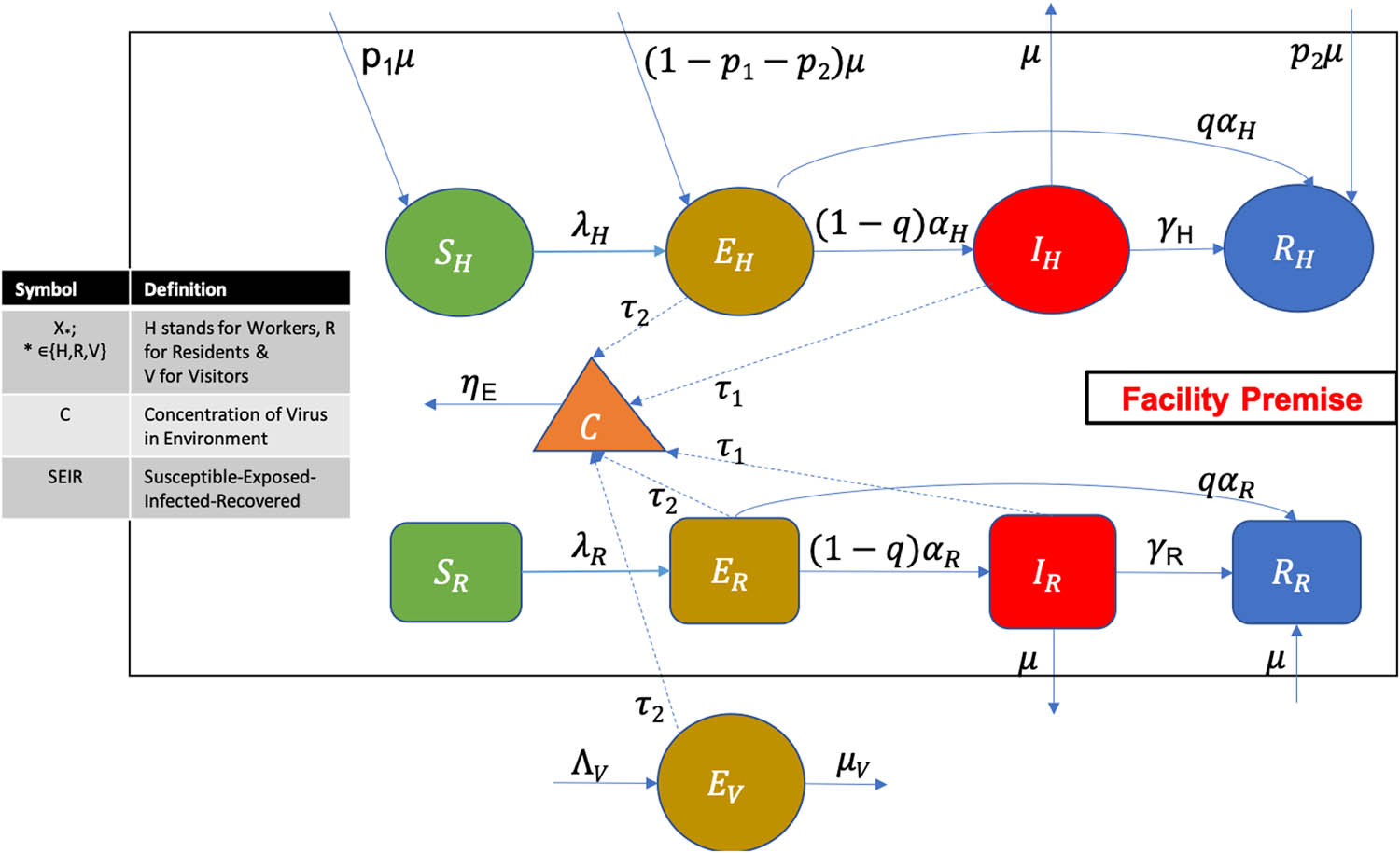
Schematic diagram of a SEIR type epidemic model framework where the subscript
In particular, the model assumes homogeneous mixing among three distinct sub-populations: staff, residents, and visitors, recognizing that the different roles each plays in disease transmission (Table 1). The model acknowledges the transmission of COVID-19 not only through direct person-to-person contact but also via contaminated environmental surfaces, introducing a novel aspect of environmental transmission dynamics. This incorporation is crucial, given the virus’s ability to remain viable on surfaces for extended periods, posing an indirect transmission route. Also, the model presumes that individuals who have recovered from COVID-19 do not get reinfected during the study period, simplifying the dynamics into a SEIR framework. Super-spreading events are considered in varying degrees across different cases within the model, specifically highlighting scenarios where either healthcare staff or residents contribute disproportionately to transmission due to high contact rates or pathogen load.
where I represents the infected class of residents as well as healthcare staff and
The denominator in the term reflect total population available for mixing. For example,
Suppose
Case 1: We assume no super spreading either through infected residents or infected staff,
(5)Case 2: We assume super spreaders are among infected residents only. Since residents are considered vulnerable population, we assume that pathogen load in
(6)Case 3: We assume super spreading among healthcare workers. Since healthcare workers are considered most mobile individuals, we can assume that their contacts are happening at much higher level. That is,
(7)
Variables and parameters used in modeling
| Parameter | Description (Unit) | Estm. & Ref. |
|---|---|---|
|
|
Per-capita hospitalization rate | 1/5 days [10] |
|
|
Infection force for facility residents | |
|
|
Infection force for healthcare personnel | |
|
|
Fraction of staff who are susceptible to COVID-19 after hospitalization | 0.2 (varied) |
|
|
Fraction of staff who recovered from COVID-19 after hospitalization | 0.8 (varied) |
|
|
Fraction of staff who were mildly symptomatic and recovered from COVID-19 | 0.38 [10] |
|
|
Rate per-capita at which an infected asymptomatic residents become symptomatic | 1/6 days [10] |
|
|
For Case 2: Rate per-capita at which an infected asymptomatic residents become symptomatic | 1/6 days [10] |
|
|
For Case 3: Rate per-capita at which an infected asymptomatic residents become symptomatic | 1/6 days [10] |
|
|
Recovery rate per-capita for the asymptomatic or mildly infected healthcare staff | 1/10 days - 1/14 days [10,36] |
|
|
Recovery rate for the asymptomatic or mildly infected residents | 1/10 - 1/14 days [10,36] |
|
|
Viral shedding rate of infected symptomatic residents and healthcare staff | 1 unit inoculum per day per capita [33] |
|
|
Viral shedding rate of infected asymptomatic or mildly infected residents and healthcare staff | 2.71 unit inoculum per day per capita [33] |
|
|
Decay rate of the virus | 1/2 days [33] |
|
|
Incoming rate of infected visitors | 20 visitors/day (varied) |
|
|
Environmental transmission rate |
|
|
|
For Case 2: Environmental transmission rate |
|
|
|
For Case 3: Environmental transmission rate |
|
|
|
Per-capita disease transmission rate | 1.9 (varied) (Estimated) |
|
|
Proportion of symptomatically infected residents who are super-spreaders | 0.2 [2,32] |
|
|
Proportion of infected healthcare workers who are super-spreaders | 0.2 [2,32] |
|
|
Reduction in infectivity for regular
|
0.25 [32] |
|
|
For Case 3: Reduction in infectivity for regular
|
0.375 |
|
|
Number of residents | 200 |
|
|
Number of healthcare staff | 100 |
|
|
Number of visitors | 50 |
|
|
Weight for infected residents | 163.13 |
|
|
Weight for infected healthcare staff | 1026.14 |
|
|
Weight for exposed healthcare staff | 163.13 |
|
|
Weight for exposed residents | 217.50 |
|
|
Relative cost for wearing masks | 234 |
|
|
Relative cost for cleaning surfaces | 4,032 |
In each of these cases, we consider three possible ways for the outbreak to begin. First, since the healthcare workers are moving in and out of the facility, we assume a case where the outbreak begins with an exposed healthcare worker. Second, since the residents are a vulnerable population, we assume a case in which the outbreak begins with an exposed resident. Third, since visitors move into the facility from outside, we assume a case where the outbreak begins with an exposed visitor. For the parameter estimation, the assumptions include:
Super-spreading events: The model distinguishes between scenarios with and without super-spreading events. Specifically, it assumes the presence of super-spreaders only in Cases 2 and 3, directly affecting the rate (
Proportion of symptomatically infected residents: It assumes that a higher proportion of symptomatically infected residents harbors a high pathogen load in Cases 2 and 3, affecting the calculation of (
Estimation of (
Adjustments for super-spreader dynamics: In Case 3, the model further adjusts its parameters to account for the possibility that not only the infected but also the exposed healthcare population could act as super-spreaders. This reflects consideration of how disease dynamics can be influenced by different population segments.
2.2 Sensitivity analysis
The purpose of assessing the local sensitivity of
Define the normalized sensitivity index of the basic reproduction number
The details of the sensitivity analysis of the parameters is shown in Figure 2. For example, in Figure 2, consider the sensitivities

Using sensitivity analysis, the impact of each parameter on R 0 is determined. The sensitivity index of the parameters for the reproductive number, R 0, is evaluated across three cases: (a) Case 1 – no super-spreading, (b) Case 2 – super-spreaders present only among infected residents, and (c) Case 3 – super-spreading occurs among healthcare workers.
3 Framework with objective function and controls
The aim of the optimal control framework is to minimize the number of infected individuals over a finite time interval
with appropriate initial conditions [24].
For this implementation, we compare using two optimal control strategies, one is using a quadratic optimal control and the other is linear optimal control. Hence, it is more efficient to reduce the impact of a disease using nonpharmaceutical interventions.
3.1 Quadratic control
The appropriate functional to be minimized is given by
3.2 Linear control
The appropriate functional to be minimized is given by
4 Analysis
4.1 Reproductive number
We use the next-generation matrix method, to calculate the reproductive number of our model. The infection-related compartments of the model include
The reproduction number of the model is (detailed steps of computation of next-generation matrix are shown in Appendix).
For cases 1, 2, and 3, respectively, considering
4.2 Existence conditions in case of quadratic control
The goal is to minimize the exposed and infectious population, and the cost of implementing the control by nonpharmaceutical intervention using possible minimal control variables
subject to system (A14), (A15), and (A16), where the control set is defined by
We construct the Hamiltonian:
Theorem 4.1
There exist the optimal control
satisfying the transversality conditions,
The Hamiltonian
Solving for the optimal condition
Similar results are also derived for the other cases (see Appendix).
4.3 Existence conditions in case of linear control
The goal is to minimize the exposed and infectious population, and the cost of implementing the control by nonpharmaceutical intervention using possible minimal control variables
subject to system (A14), (A15), (A16), where the control set is defined by
We construct the Hamiltonian
satisfying the transversality conditions,
The Hamiltonian
This a bang-bang control due to the solutions, where
and we have the following:
and when is
5 Numerical results
5.1 Model parameter estimates of the dynamical system
Relevant data are identified for estimation of the parameters in the model. The values for the parameters used in the simulations are shown in Table 2. The model flow chart is shown in Figure 1, which includes transmission of COVID-19 in a closed-contact facility. The model captures a coupled dynamics between three subpopulation (staff, the residents, and the visitors of the facility) and incorporates infection from infectious individuals and through environment. In the model, we assume that (i) populations of staff, residents, and visitors mix homogeneously in a facility and (ii) the infectivity of resident patients relative to infected staff is constant over time. The estimates of parameters are taken from literature and collected in Table 2.
We also consider certain specific scenarios by choosing selected values of
5.2 Simulation of dynamical system (i.e., optimal control system without objective function
This section studies the system’s evolution numerically with and without incorporating the two optimal nonpharmaceutical interventions to prevent COVID-19. The evolution of the system defined by the state model (described by equations (1)–(4)) without any control strategies is presented for the three cases described in Section 2.1. The first case is shown in Figure 3. We study the model for 70 days for the population of residents and healthcare staff based on parameter values given in Table 2. Cases 2 and 3 are shown in Figures A1 and A2 in the Appendix. For the three cases, we notice that it roughly takes 20–30 days for the infection peak to come down. We note here that the recovered class is not considered immune. We apply different initial conditions proposed in Section 2.1 to all three cases. These initial conditions differ from each other just in the exposed population where the outbreak starts. However, no significant change is observed (variation around
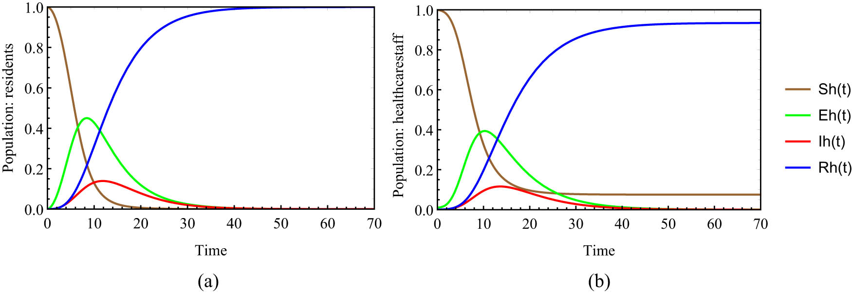
Case 1: State model simulation (described by equations (1)–(2)) without applying any control for (a) resident and (b) healthcare staff populations based on the parameters of Table 2. Here,
Figure 4 indicates the infected and exposed populations for the three cases. The third case indicates a higher peak than in the other cases, and it is reached earlier for both residents and healthcare staff. This is due to the assumption that super-spreading event is considered in the healthcare worker’s population in the third case. For cases 1 and 2, the maximum is reached at day 10, with a total of infected plus exposed populations of 50 and 53 people, respectively. In Case 3, the maximum of the peak is reached at day 6 with a total of 68 people; this means an increase of 36% with respect to Case 1.

Cases 1, 2, 3: State model simulations without control for (a) infected and exposed residents and (b) infected and exposed healthcare staff based on the parameters of Table 2. Here,
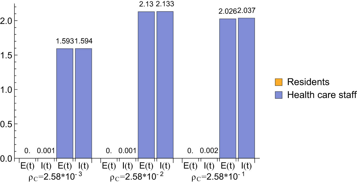
Figure 5 shows how the infected population of residents change according to different values of

Case 1: State model simulation with different values of
Figure 6 shows the exposed population of infected healthcare staff as a function of time for different proportions (

The exposed healthcare workers are plotted as a function of time for different proportions
5.3 Estimates of parameters in objective function
The value for the weight coefficients
Weights used in the optimal control simulations
| Parameter | Description (cost per person per day) | Estm. |
|---|---|---|
|
|
Weight constant of the exposed residents | 256.54 [1] |
|
|
Weight constant of the infected residents | 1026.14 [1] |
|
|
Weight constant of the exposed healthcare staff | 76.13 [1] |
|
|
Weight constant of the infected healthcare staff | 304.50 [1] |
|
|
Measure of the relative cost for interventions like masks | 234 [14] |
|
|
Measure of the relative cost for interventions like cleaning surfaces | 896 [14] |
We also estimate
There are different types of functional forms for the control variable
5.4 Computation of the optimal control
The forward-backward sweep method was used to numerically solve the dynamic control system (as in [25]). First, an initial guess of the control parameters were selected (
5.4.1 Optimal control in case of quadratic objective function
The optimal control strategy is obtained for the quadratic objective function, and the results are shown in Figures 7 and 8. In Figure 7, controls

The controls for the quadratic objective function,

Case 1: Evolution of the exposed and infected populations with and without control based on the parameters of Table 2.
The evolution of the exposed and infected residents and healthcare staff taken together, in the presence and absence of the two control strategies, shows the effectiveness of the controls to drastically reduce the infection peak and epidemic size. The optimal controls decreases the infection peak as

Difference in epidemic sizes of the resident and healthcare staff populations with optimal controls compared to no controls.
We notice that control
5.4.2 Optimal control in case of linear objective function
The same numerical method was used to solve optimal control problem with linear objective function [25]. Figure 11 shows the optimal control strategies, where controls

The control

The controls for the linear objective function,
In Figure 12, we present the evolution of the infected and exposed populations for residents and for healthcare staff when there is no control (solid curve) and when control is introduced (dotted curve). Figure 13 shows the difference in epidemic sizes between controlled and uncontrolled system. For example, the reduction in infection peak for low, medium, and high

Case 1: Evolution of the exposed and infected populations with and without control based on the parameters of Table 2 for different values of

Relative difference in epidemic sizes for resident and for healthcare staff populations under controls with respect to no controls. Each bar represents different values of

Exposed and infected populations of residents and healthcare staff together. Simulations are based on the parameters of Table 2.
In the scenario, we notice that controls
6 Discussion
In the present study, we propose a dynamical system-based model for a long-term care facility, which captures highly transmissible disease such as COVID-19, to evaluate effective prevention and intervention programs for vulnerable population. The emphasis is on the evaluation of control policies, timely identification, and exclusion of potentially infected residents and staff members, while ensuring early recognition and implementation of appropriate nonpharmaceutical interventions. Through our analysis, we show the trade off between disease burden and prevention cost via adaptive cost-effectiveness analysis. Three cases were developed for the model that includes super-spreading events by healthcare staff (Case 3), residents (Case 2), or neither (Case 1). We identified data that may be relevant to estimate model parameters. An optimal control method is described to estimate cost parameters used in the model.
The results suggest that the estimates of the basic reproduction number for Case 1 is significantly less than the estimates in other two cases for the same values of transmission coefficient,
The numerical simulations shows less influence of the initial conditions, that is, introducing the first arrival infection in the residents, visitors, or staff populations has low impact on the dynamics. More attention should be given to the time application of selective nonpharmaceutical interventions. The simulations were carried out using two different types of type objective functions: quadratic and linear. Using quadratic objective functions, as indicated by Figure 7, wearing masks should be a priority during whole epidemic, while cleaning virus-contaminated surfaces in a long-term facility is crucial at the beginning of the epidemic as community transmission rate may be high at the time of outbreak realization. However, this last situation may be altered if the concentration of the virus in the environment is significantly large and high transmission from surfaces is possible. That is, if the concentration of virus in environment increases, then cleaning surfaces are also need to considered as optimal strategy (Figure 10). The simulations were also carried out using variations in two specific parameters:
Close-contact places such as nursing homes, old-age homes, long-term facilities, and vacation cruises have been found to be high-risk and high-morbidity places worldwide during the COVID-19 outbreaks. Our model captures a coupled dynamics between three sub-populations (staff, the residents, and the visitors) and incorporates infection from infectious individuals and through the environment. We have observed here how super spreaders considered in healthcare staff (Case 3) can increase the peak of the infected population more than super spreaders among the resident population due to higher mobility among the healthcare staff. The analysis of each of the three sub-populations is important and differs with respect to the averaged behavior of the whole population. We showed existence of optimal solution for the model for all the three cases; however, numerical scenarios were considered for Case 1. We have also highlighted the data sets and procedures to estimates epidemic and economic parameters. Our model shows how incorporation of the nonpharmaceutical strategies decreases the peak of the infected population and altered disease dynamics. The study stresses that the control effort are directly proportional to known transmission pathways, and potential for different types of super-spreading events.
There are several other limitations to our analysis.We utilized the most up-to-date biological parameters for SARS-CoV-2 based on current available evidence; however, these values may need to be refined as more comprehensive and diverse data become accessible. Through fitting to various datasets to infer model parameters and conducting sensitivity analyses on critical areas of uncertainty, we have endeavored to optimize the utilization of the available evidence regarding SARS-CoV-2 transmission dynamics.
The explicit structure of the visiting and community population was not captured in the study. However, we employed reasonable estimates of connectivity and risk for visitors to account for the influence of family members and community infections. These estimates have demonstrated favorable correspondence with other similar assessments in the literature and have contributed to a reasonable risk assessment for COVID-19 based on different scenarios.
We assumed that the latent period is equivalent to the incubation period, meaning that individuals become infectious and symptomatic simultaneously, and that all infected individuals will eventually exhibit symptoms. However, evidence suggests that transmission of SARS-CoV-2 can occur even with few reported symptoms [31]. Hence, we conducted sensitivity analysis to explore the possibility of transmission occurring at different times during the incubation period. Additionally, our analysis incorporated estimates of individual-level variation in transmission for SARS to illustrate potential dynamics. Nonetheless, the precise extent of such variation for SARS-CoV-2 remains unclear [31].
In some modeling studies before COVID-19, model outcomes have been cross-checked against alternative data. For instance, [12] conducted a comparison of model forecasts regarding human immunodeficiency virus (HIV) prevalence and treatment coverage with outcomes from a national survey in South Africa, and their analysis revealed that while some model estimates were distributed around the survey mean, others showed systematic differences, with the majority of the modeled estimates falling on one side of the survey confidence interval. Consequently, while combining results from multiple models may mitigate the impact of mis-specification by any individual model, aggregated outcomes remain susceptible to systematic biases.
As additional more precise data becomes available, these estimates can be refined. In spite of that, the model in this study serves as a flexible tool that can be readily extended to incorporate new data as it becomes available. Our findings indicate significant variation in SARS-CoV-2 transmission over time and suggest a potential decline in transmission coinciding with the implementation of various control measures.
7 Conclusion
The combination of a vulnerable population, displaying nonspecific and atypical COVID-19 symptoms, along with staffing shortages due to viral infections, and limited access to rapid testing and personal protective equipment, has created a significant challenge in places like nursing homes. This study delves into the cost-effectiveness of intervention strategies for this vulnerable population in close-contact environments, aiming to identify optimal approaches amidst varying epidemiological conditions and the trade-off between disease burden and prevention cost.
We observed that the presence of a super-spreader among healthcare workers leads to a notably higher peak in the number of infected cases compared to situations where super-spreaders are limited to residents. This may be attributed to the frequent social interactions of residents with healthcare workers, particularly in medication rooms and nursing home kitchens. In fact, one such research indicates that disregarding hand sanitization by healthcare workers resulted in a quarter of residents in nursing homes becoming infected [19]. However, adequate staffing levels among healthcare workers are also crucial for effectively caring for the vulnerable population in close-contact settings. Studies have shown that nursing homes with staffing levels below the recommended minimum standard have a significantly higher probability of resident COVID-19 infections [17].
In our results, we observed that cleaning surfaces is an effective intervention at the onset of an outbreak, whereas wearing masks becomes more optimal once the infection has spread widely and population behaviors have shifted. However, strict enforcement of mask usage, routine cleaning and disinfection protocols, and dissemination of health protection information are essential for raising awareness. Collaborative efforts to adhere to these guidelines are crucial for preventing illness by minimizing exposure to pathogens. It is important to ensure that masks or face shields are properly fitted for individuals of different sizes to prevent air leaks and reduce the risk of infection.
In this study, the analysis has studied certain biases associated with parameter inference using mechanistic mathematical model and sensitivity analysis. The findings illustrate that overlooking statistical inference may result in parameter estimates and model predictions that are overly precise and systematically biased. Many of the considerations discussed here relate to how a model’s outcomes are validated. The biases in modeling differ significantly when assessing novel and rapidly evolving policies, such as those for COVID-19 control, compared to evaluating established policies and interventions. With established policies, accumulated evidence often reveals the realities of routine implementation, where policy impact may be less than initially anticipated and can sometimes have adverse effects. In contrast, for new policies, the factors limiting effectiveness may not be well understood, and harmful unintended consequences may yet to be recognized. Although validating model outcomes can be challenging, it is still feasible to analyze model processes, as demonstrated in this study. One advantage of mechanistic models, compared to purely statistical models, is their attempt to replicate the underlying processes that generate observed outcomes, such as disease natural history or healthcare provision processes. This approach allows for the critique and comparison of parameters used to model these mechanisms against external data.
Acknowledgements
The corresponding author, AG, extends thanks to the AMS-Simons Research Enhancement Grants for Primarily Undergraduate Institution for supporting this research. The funders had no role in study design, data collection and analysis, decision to publish, or preparation of the manuscript.
-
Funding information: There is no financial interest to report.
-
Author contributions: The corresponding author and the last author contributed to the conceptualization and design of the study as well as drafting and revising the manuscript. They provided expert guidance on the theoretical framework and methodology, and contributed to the interpretation of the results. The first, second and the third authors have assisted in data collection, methodology and performed mathematical analysis. They were also responsible for the literature review and provided critical revisions for intellectual content. All authors have read and approved the final version of the manuscript.
-
Conflict of interest: The authors have no conflicts of interest to declare.
-
Ethical approval: This research did not require ethical approval.
-
Data availability statement: Data sharing is not applicable to this article as no datasets were generated or analysed during this work.
Appendix
A.1 Parameter estimation
The disease transmission rate,
Similarly in Case 3 (equation (7)); we use the following equation to estimate
Similarly,
Now we estimate the proportion of the virus in the environment,
By using equation (A4), we estimate
A.2 Reproductive number
Next, we will calculate the

Case 2: State model simulations without applying any control for (a) resident and (b) healthcare staff populations based on the parameters of Table 1. (a) Model simulation for resident population (equation (1)) without any control for case 2 and (b) model simulation for healthcare staff population (equation (2)) without any control for case 2.

Case 3: State model simulations without control for (a) resident and (b) healthcare staff populations based on the parameters of Table 1. (a) Model simulation for resident population (equation (1)) without any control for case 3 and (b) model simulation for healthcare staff population (equation (2)) without any control for case 3.
Taking the partial derivatives of
These matrices are calculated and then evaluated at the DFE:
To calculate the next-generation matrix, we multiply the
where
where
A.3 State model without any control strategies numerical simulations
For next subsection, we compare using two optimal control strategies, one is using a quadratic optimal control and the other is linear optimal control. Due to which is more efficient to reduce the impact of a disease using nonpharmaceutical interventions.
A.3.1 Quadratic optimal control
Figure A3 shows the exposed and infected populations simulations with and without the control, and Figure A4 shows the relative difference of Figure A3, and Figure A5 is plotted the control

Case 1: Exposed and infected populations simulations with and without control based on the parameters of Table 1 for different values (low, medium, high) of

Comparative values of the area under the curve of each line in Figure A3.

The control
A.3.2 Linear optimal control
Figure A6 shows the exposed and infected populations simulations with and without the control, and in Figure A7 shows the relative difference of Figure A3, all the previous figures are for the three values of
where
with appropriate initial conditions [24]. The appropriate functional to be minimized is given by
subject to the state system given by (A7), (A8), and (A9). The goal is to minimize the exposed and infectious population, and the cost of implementing the control by nonpharmaceutical intervention using possible minimal control variables

Case 1: Exposed and infected populations simulations with with and without control based on the parameters of Table 1 for different values (low, medium, high) of
Comparative values of the area under the curve of each line in Figure A6.

subject to system (A14), (A15), and (A16), where the control set is defined by
We construct the Hamiltonian:
Theorem A.1
There exist the optimal control
satisfying the transversality conditions,
The Hamiltonian
By solving for the optimal condition
where
with appropriate initial conditions [24]. The appropriate functional to be minimized is given by
subject to the state system given by (A14), (A15), and (A16). The goal is to minimize the exposed and infectious population, and the cost of implementing the control by nonpharmaceutical intervention using possible minimal control variables
subject to system (A14), (A15), and (A16), where the control set is defined by
The existence of optimal controls is guaranteed by standard results in control theory, i.e., the state system satisfies the Lipshitz property with respect to the state variables and
Theorem A.2
There exist the optimal control
satisfying the transversality conditions,
The Hamiltonian
By solving for the optimal condition
References
[1] Lee BY. (2020, May 4). Treating coronavirus will cost U.S. billions–and guess who will pay, MarketWatch. Retrieved September 30, 2020, [Online] Available: https://www.marketwatch.com/story/treating-coronavirus-will-cost-us-billions-and-guess-who-will-pay-2020-05-04.Search in Google Scholar
[2] Adam, D. C., Wu, P., Wong, J. Y., Lau, E. H., Tsang, T. K., Cauchemez, S., et al. (2020). Clustering and superspreading potential of sars-cov-2 infections in Hong Kong. Nature Medicine, 26(11), 1714–1719. 10.1038/s41591-020-1092-0Search in Google Scholar PubMed
[3] Althouse, B. M., Wenger, E. A., Miller, J. C., Scarpino, S. V., Allard, A., Hébert-Dufresne, L., et al. (2020). Superspreading events in the transmission dynamics of SARS-CoV-2: Opportunities for interventions and control. PLoS Biology, 18(11), 3000897. 10.1371/journal.pbio.3000897Search in Google Scholar PubMed PubMed Central
[4] Arriola, L. and Hyman, J. (2007). Being Ssensitive to Uncertainty. Computing in Science & Engineering, 9(2), 10–20. 10.1109/MCSE.2007.27Search in Google Scholar
[5] Arriola, L. and Hyman, J. (2009). Sensitivity analysis for uncertainty quantication in mathematical models. In Mathematical and Statistical Estimation Approaches in Epidemiology, Dordrecht: Springer Netherlands.10.1007/978-90-481-2313-1_10Search in Google Scholar
[6] Berklan, J. M. (2020, April 9). Analysis: PPE costs increase over 1,000% during COVID-19 crisis. McKnight's Long-Term Care News. https://www.mcknights.com/news/analysis-ppe-costs-increase-over-1000-during-covid-19-crisis/.Search in Google Scholar
[7] Blayneh, K., Cao, Y., and Kwon, H.-D. (2009). Optimal control of vector-borne diseases: treatment and prevention. Discrete and Continuous Dynamical Systems-B, 11(3), 587. 10.3934/dcdsb.2009.11.587Search in Google Scholar
[8] Carlos, W. G., Dela Cruz, C. S., Cao, B., Pasnick, S., and Jamil, S. (2020). Novel Wuhan (2019-nCoV) coronavirus. Am J Respir Crit Care Med, 201 P7–P8. 10.1164/rccm.2014P7Search in Google Scholar PubMed
[9] CDC (2019). Prioritizing covid-19 contact tracing mathematical modeling methods and findings. Centers for Disease Control and Prevention. Search in Google Scholar
[10] Centers for Disease Control and Prevention. (2020). COVID-19 pandemic planning scenarios. https://www.cdc.gov/coronavirus/2019-ncov/hcp/planning-scenarios.html.Search in Google Scholar
[11] Chen, M. K., Chevalier, J. A., and Long, E. F. (2021). Nursing home staff networks and covid-19. Proceedings of the National Academy of Sciences, 118(1), e2015455118. 10.1073/pnas.2015455118Search in Google Scholar PubMed PubMed Central
[12] Eaton, J. W., Bacaër, N., Bershteyn, A., Cambiano, V., Cori, A., Dorrington, R. E., et al. (2015). Assessment of epidemic projections using recent HIV survey data in South Africa: a validation analysis of ten mathematical models of HIV epidemiology in the antiretroviral therapy era. The Lancet Global Health, 3(10), e598–e608. 10.1016/S2214-109X(15)00080-7Search in Google Scholar PubMed
[13] Barker, J. (2020, April 7). Amid shortages, using PPE according to CMS guidelines could cost nursing homes $10K a day – or more. Skilled Nursing News. https://skillednursingnews.com/2020/04/amid-shortages-using-ppe-according-to-cms-guidelines-could-cost-nursing-homes-10k-a-day-or-more/ Accessed on May 1, 2023.Search in Google Scholar
[14] Zimmet M, Silverberg J, Stawis A, Greenfield M. (2020). Analysis of emergency, unfunded, marginal PPE costs incurred by skilled nursing facilities and assisted living centers treating COVID-19 patients. CNN, Accessed September 30, 2020. [Online]. Available: https://cdn.cnn.com/cnn/2020/images/04/16/.Search in Google Scholar
[15] Ghinai, I., McPherson, T. D., Hunter, J. C., Kirking, H. L., Christiansen, D., Joshi, K., et al. (2020). First known person-to-person transmission of severe acute respiratory syndrome coronavirus 2 (SARS-CoV-2) in the USA. The Lancet. 10.1016/S0140-6736(20)30607-3Search in Google Scholar PubMed PubMed Central
[16] Hageman, J. R. (2020). The coronavirus disease 2019 (COVID-19). Pediatric Annals, 49(3), e99–e100. 10.3928/19382359-20200219-01Search in Google Scholar PubMed
[17] Harrington, C., Ross, L., Chapman, S., Halifax, E., Spurlock, B., and Bakerjian, D. (2020). Nurse staffing and coronavirus infections in California nursing homes. Policy, Politics, and Nursing Practice, 21(3), 174–186. 10.1177/1527154420938707Search in Google Scholar PubMed
[18] Hull, R. (2022). Locked. In: Impact of Social Isolation and Loneliness on Residents in Long-Term Care Facilities. PhD thesis, University of Pittsburgh. Search in Google Scholar
[19] Hüttel, F. B., Iversen, A.-M., Bo Hansen, M., Kjær Ersbøll, B., Ellermann-Eriksen, S., and Lundtorp Olsen, N. (2021). Analysis of social interactions and risk factors relevant to the spread of infectious diseases at hospitals and nursing homes. Plos One, 16(9), e0257684. 10.1371/journal.pone.0257684Search in Google Scholar PubMed PubMed Central
[20] Kimball, A., Hatfield, K. M., Arons, M., James, A., Taylor, J., Spicer, K., et al. (2020). Asymptomatic and presymptomatic sars-cov-2 infections in residents of a long-term care skilled nursing facility king county, Washington, march 2020. Morbidity and Mortality Weekly Report, 69(13), 377. 10.15585/mmwr.mm6913e1Search in Google Scholar PubMed PubMed Central
[21] Kuupferschmidt, K. (2020). Why do some covid-19 patients infect many others, wheras most don’t spread the virus at all? Science Magazine.org, 1(1), 1. Search in Google Scholar
[22] Kwok, K. O., Leung, G. M., Lam, W. Y., and Riley, S. (2007). Using models to identify routes of nosocomial infection: a large hospital outbreak of SARS in Hong Kong. Proceedings of the Royal Society B: Biological Sciences, 274(1610), 611–618. 10.1098/rspb.2006.0026Search in Google Scholar PubMed PubMed Central
[23] Lashari, A. A. and Zaman, G. (2012). Optimal control of a vector borne disease with horizontal transmission. Nonlinear Analysis: Real World Applications, 13(1), 203–212. 10.1016/j.nonrwa.2011.07.026Search in Google Scholar
[24] Lee, S., Morales, R., and Castillo-Chavez, C. (2011). A note on the use of influenza vaccination strategies when supply is limited. Math. Biosci. Eng, 8(1), 171–182. 10.3934/mbe.2011.8.171Search in Google Scholar PubMed
[25] Lenhart, S. and Workman, J. T. (2007). Optimal control applied to biological models. New York: Chapman and Hall/CRC.10.1201/9781420011418Search in Google Scholar
[26] Lewis, D. (2021). Superspreading drives the covid pandemic-and could help to tame it. Nature, 590, 544–546. 10.1038/d41586-021-00460-xSearch in Google Scholar PubMed
[27] McMichael, T. M., Clark, S., Pogosjans, S., Kay, M., Lewis, J., Baer, A., et al. (2020). COVID-19 in a long-term care facility king county, Washington, February 27-March 9, 2020. Morbidity and Mortality Weekly Report, 69(12), 339. 10.15585/mmwr.mm6912e1Search in Google Scholar PubMed PubMed Central
[28] Moore, S. E. and Okyere, E. (2020). Controlling the transmission dynamics of covid-19. arXiv: http://arXiv.org/abs/arXiv:2004.00443. Search in Google Scholar
[29] Nishiura, H., Oshitani, H., Kobayashi, T., Saito, T., Sunagawa, T., Matsui, T., et al. (2020). Closed environments facilitate secondary transmission of coronavirus disease 2019 (covid-19). MedRxiv. doi: 10.1101/2020.02.28.20029272.Search in Google Scholar
[30] Nuño, M., Reichert, T. A., Chowell, G., and Gumel, A. B. (2008). Protecting residential care facilities from pandemic influenza. Proceedings of the National Academy of Sciences, 105(30), 10625–10630. 10.1073/pnas.0712014105Search in Google Scholar PubMed PubMed Central
[31] Rothe, C., Schunk, M., Sothmann, P., Bretzel, G., Froeschl, G., Wallrauch, C., et al. (2020). Transmission of 2019-ncov infection from an asymptomatic contact in Germany. New England journal of medicine, 382(10), 970–971. 10.1056/NEJMc2001468Search in Google Scholar PubMed PubMed Central
[32] Stein, R. A. (2011). Super-spreaders in infectious diseases. International Journal of Infectious Diseases, 15(8), e510–e513. 10.1016/j.ijid.2010.06.020Search in Google Scholar PubMed PubMed Central
[33] Stutt, R. O. J. H., Retkute, R., Bradley, M., Gilligan, C. A., and Colvin, J. (2020). A modelling framework to assess the likely effectiveness of facemasks in combination with lock-down in managing the covid-19 pandemic. Proceedings of the Royal Society A: Mathematical, Physical and Engineering Sciences, 476(2238), 20200376. 10.1098/rspa.2020.0376Search in Google Scholar PubMed PubMed Central
[34] Tobolowsky, F. A., Gonzales, E., Self, J. L., Rao, C. Y., Keating, R., Marx, G. E., et al. (2020). COVID-19 outbreak among three affiliated homeless service sites-king county, Washington, 2020. Morbidity and Mortality Weekly Report, 69(17), 523. 10.15585/mmwr.mm6917e2Search in Google Scholar PubMed PubMed Central
[35] Wang, R.-H., Jin, Z., Liu, Q.-X., van de Koppel, J., and Alonso, D. (2012). A simple stochastic model with environmental transmission explains multi-year periodicity in outbreaks of Avian flu. PLoS One, 7(2), e28873. 10.1371/journal.pone.0028873Search in Google Scholar PubMed PubMed Central
[36] WHO Headquarters (HQ). (2020). Report of the who-china joint mission on coronavirus disease 2019 (covid-19). World Health Organization (Feb 2020), [Online]. Available: https://www.who.int/publications/i/item/report-of-the-who-china-joint-mission-on-coronavirus-disease-2019-(covid-19).Search in Google Scholar
© 2024 the author(s), published by De Gruyter
This work is licensed under the Creative Commons Attribution 4.0 International License.
Articles in the same Issue
- Special Issue: Recent Trends in Mathematical Biology – Theory, Methods, and Applications
- Editorial for the Special Issue: Recent trends in mathematical Biology – Theory, methods, and applications
- Behavior of solutions of a discrete population model with mutualistic interaction
- Influence of media campaigns efforts to control spread of COVID-19 pandemic with vaccination: A modeling study
- Optimal control and bifurcation analysis of SEIHR model for COVID-19 with vaccination strategies and mask efficiency
- A mathematical study of the adrenocorticotropic hormone as a regulator of human gene expression in adrenal glands
- On building machine learning models for medical dataset with correlated features
- Analysis and numerical simulation of fractional-order blood alcohol model with singular and non-singular kernels
- Stability and bifurcation analysis of a nested multi-scale model for COVID-19 viral infection
- Augmenting heart disease prediction with explainable AI: A study of classification models
- Plankton interaction model: Effect of prey refuge and harvesting
- Modelling the leadership role of police in controlling COVID-19
- Robust H∞ filter-based functional observer design for descriptor systems: An application to cardiovascular system monitoring
- Regular Articles
- Mathematical modelling of COVID-19 dynamics using SVEAIQHR model
- Optimal control of susceptible mature pest concerning disease-induced pest-natural enemy system with cost-effectiveness
- Correlated dynamics of immune network and sl(3, R) symmetry algebra
- Variational multiscale stabilized FEM for cardiovascular flows in complex arterial vessels under magnetic forces
- Assessing the impact of information-induced self-protection on Zika transmission: A mathematical modeling approach
- An analysis of hybrid impulsive prey-predator-mutualist system on nonuniform time domains
- Modelling the adverse impacts of urbanization on human health
- Markov modeling on dynamic state space for genetic disorders and infectious diseases with mutations: Probabilistic framework, parameter estimation, and applications
- In silico analysis: Fulleropyrrolidine derivatives against HIV-PR mutants and SARS-CoV-2 Mpro
- Tangleoids with quantum field theories in biosystems
- Analytic solution of a fractional-order hepatitis model using Laplace Adomian decomposition method and optimal control analysis
- Effect of awareness and saturated treatment on the transmission of infectious diseases
- Development of Aβ and anti-Aβ dynamics models for Alzheimer’s disease
- Compartmental modeling approach for prediction of unreported cases of COVID-19 with awareness through effective testing program
- COVID-19 transmission dynamics in close-contacts facilities: Optimizing control strategies
- Modeling and analysis of ensemble average solvation energy and solute–solvent interfacial fluctuations
- Application of fluid dynamics in modeling the spatial spread of infectious diseases with low mortality rate: A study using MUSCL scheme