Dynamics of an eco-epidemic model with Allee effect in prey and disease in predator
-
Bipin Kumar
 and
Rajesh Kumar Sinha
and
Rajesh Kumar Sinha

Abstract
In this work, the dynamics of a food chain model with disease in the predator and the Allee effect in the prey have been investigated. The model also incorporates a Holling type-III functional response, accounting for both disease transmission and predation. The existence of equilibria and their stability in the model have also been investigated. The primary objective of this research is to examine the effects of the Allee parameter. Hopf bifurcations are explored about the interior and disease-free equilibrium point, where the Allee is taken as a bifurcation point. In numerical simulation, phase portraits have been used to look into the existence of equilibrium points and their stability. The bifurcation diagrams that have been drawn clearly demonstrate the presence of significant local bifurcations, including Hopf, transcritical, and saddle-node bifurcations. Through the phase portrait, limit cycle, and time series, the stability and oscillatory behaviour of the equilibrium point of the model are investigated. The numerical simulation has been done using MATLAB and Matcont.
1 Introduction
In ecology and eco-epidemiology, mathematical modelling plays an important role. In the current situation, the world suffers from various epidemic crises like COVID, dengue, plague, flu, and various zoonotic diseases. Eco-epidemiology is a relatively new area in mathematical modelling that deals with ecological and epidemiological issues simultaneously [10,31]. Our understanding of epidemic models has greatly improved as a result of the innovative work done by Kermack and McKendrick, opening the door for the investigation of a newly created interdisciplinary area called eco-epidemiology [11]. To better understand the dynamics of disease within communities, this field connects components of ecology and epidemiology. There is a wealth of literature in the field of human-related epidemiology that applies the ideas of the Kermack-McKendrick model. Research on diseases like HIV [3], rabies [27], the mumps virus [24], and the SARS-coronavirus [4] are a few famous examples. These research have improved our knowledge of how diseases spread and are controlled in human societies. By creating mathematical models that depict the spread of diseases among interacting populations, Hadeler and Freedman [17] have significantly improved our understanding of the subject. Their research has illuminated how illnesses might spread across intricate ecological networks. By examining subjects like species persistence and Hopf bifurcation within epidemic models, Mukherjee [25] has added to our understanding. This study has shed important light on the mechanisms of disease persistence and the crucial junctures at which important shifts in ecological and epidemiological systems take place. Ecological species sizes are important in ecological studies and are influenced by a variety of ecological and epidemiological factors. Predatory behaviour, intraspecific and interspecific competition, and various types of species interaction are the ecological aspects. The transmission of infectious diseases is one of the major epidemiological issues [28]. Researchers are interested in studying infectious diseases in their natural environment. The effects of infectious diseases should be considered in the study of dynamical systems [26]. The first predator-prey model was given by Lotka and Volterra for two species and is the simplest model of predator-prey interactions. The predator-prey model was developed independently by Lotka in 1925 and Volterra in 1926 [9,37], the general form of the simplest Lotka-Volterra model is given as follows:
where
where
The Allee effect has currently received considerable attention in research communities due to its significant effect on population dynamics. The phenomenon, often referred to as the Allee effect [2], explains the positive association between the per capita growth rate and population density. The emergence of this phenomenon may be related to many different factors, including challenges in locating compatible partners in territories with low populations, a rise in susceptibility to predation, negative effects resulting from mating among closely related individuals, the insufficient presence of defensive mechanisms against predators, and other contributing factors. The Allee effect is often classified into two primary categories: strong and weak instances. The phenomenon referred to as a significant Allee effect, sometimes termed critical dispensation, occurs when a population attains a critical size or threshold. Once the barrier has been overcome, the per capita growth rate transitions from negative to positive and gradually approaches the carrying capacity. On the other hand, the weak Allee effect does not demonstrate a discernible threshold. Both manifestations of the Allee effect, whether they are powerful or mild, have noteworthy implications for the dynamics of populations. The Allee concept is briefly discussed in the studies by Arancibia-Ibarra and Flores [6] and Sarangi and Raw [30]. The earlier discovery has prompted the recognition that the co-occurrence of diseases and the Allee effect may have a collective influence on the sustainability and potential extinction of species. In order to clarify the biological importance of the Allee effect, notable instances such as the island fox [5] and the African wild dog [12] may be examined. The ecological and eco-epidemiological models have been published with the Allee effect by the authors [22,23,32]. These articles examine the effects of the Allee effect, which causes Hopf bifurcation and chaos.
The Allee effect can change interior equilibria and is capable of influencing internal attraction. In addition, coexistence is possible at endemic state, and under appropriate parametric situations, the infection may be suppressed [20]. The chaotic behaviour of the ecological model decreases with the increase in severity of the Allee effect [22]. Recently, researchers did work on the effects of double Allee on eco-epidemic model [30]. In predator-prey interactions, the choice of functional response plays a crucial role. The predator-prey functional response quantifies the rate at which predators consume prey per unit of time. Mathematical analyses of ecological, epidemiological, and eco-epidemiological systems rely on various functional responses, including the Holling type-I functional response [29], the Holling type-II functional response [33], and the ratio-dependent functional response, Among these, the predator-prey interaction with ratio-dependent functional response is often considered the most effective approach [7]. In this study, we investigate an eco-epidemic model that incorporates the Allee effect in prey and disease in predators. The model is initially based on the Holling type-II functional response for both predation and disease transmission, as described in the study by Shaikh and Das [32]. However, in our research, we introduce the Holling type-III functional response to the model to study its dynamics.
In this current study, we examine the dynamic behaviour of a system, specifically focusing on the examination of equilibrium states and their stability. In addition, we conduct a comprehensive analysis of bifurcation phenomena within the system. In Section 2, model formulation is discussed. In Section 3, theoretical studies such as positivity and boundedness of model 4 are studied. In Section 4, the conditions for the existence of equilibrium points have been analysed. Stability analysis about all possible equilibrium and bifurcation analysis is discussed in Section 5, in which Hopf bifurcation about the Allee parameter is obtained. In Section 6, numerical study has been done, and the dynamical properties, such as equilibria and their stability, as well as the periodic behaviour of the model, look exactly the same as the analytical study for the restricted conditions. Finally, the result discussion, the biological significance of the model, and future research have been discussed in Section 7.
2 Model description
This model is a modification of the article published by Shaikh and Das [32]. The predator is divided into two compartments, susceptible
The model with the above assumptions takes the following form:
where we take the initial restrictions
with initial condition
3 Theoretical studies of model (4)
3.1 Existence and positivity
Theorem 3.1
For the system described in equation (4) every solution associated with initial conditions where
Proof
Since the given function
where
3.2 Boundedness of the solution
Theorem 3.2
In
Proof
Let us assume
and taking the value of
If
with the theory of differential inequality (Grönwall’s inequality) [8] we obtain
and we have
4 Equilibria and their existence
The equilibrium points of system (4) are obtained by solving the equations
Using Descartes’ rule of signs, equation (6) could have two positive roots if
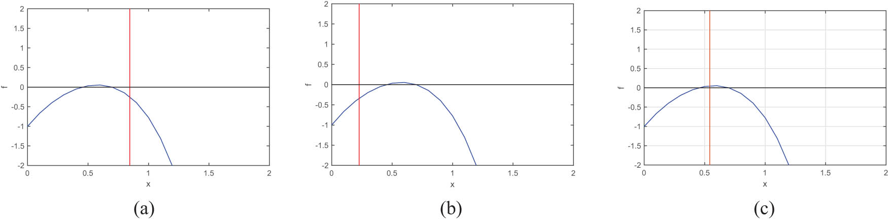
These figures show the positive roots of equation (6). The blue curve represents the graph of
5 Stability of equilibria and local bifurcation
For the local stability of the equilibrium point, we need to first find Jacobian matrix about the equilibrium point and then find the eigenvalue of the matrix. Now Jacobian matrix for model (4) is defined as follows:
where
The Jacobian matrix of model (4) about trivial equilibrium is:
where
Theorem 5.1
The equilibrium point
Proof
Jacobian matrix about
Here, all eigenvalues are negative if
Theorem 5.2
Disease-free equilibrium
Proof
The Jacobian matrix of model (4) about Disease-free equilibrium is:
where
The one eigenvalue of the above Jacobian matrix is
where both roots of equation (12) are negative if it satisfies the following conditions:
5.1 Stability analysis of coexistence equilibrium
Theorem 5.3
The interior equilibrium point of model (4) is locally asymptotically stable if the following conditions hold:
Proof
Jacobian matrix about the coexistence equilibrium:
where
The characteristic equation of the matrix is:
where
and
5.2 Bifurcation analysis
Definition 5.4
Bifurcation: Bifurcation occurs when the dynamical behaviour of a system, such as equilibrium stability and number of equilibrium, changes as a result of a small change in a parameter. The parameter at which the behaviour changes is called the bifurcation point [35].
5.2.1 Hopf bifurcation
Definition 5.5
A Hopf bifurcation is a type of local bifurcation in dynamical systems where a stable equilibrium point becomes unstable and periodic (oscillatory) behaviour emerges as a parameter changes [35].
Theorem 5.6
The model (4) shows Hopf bifurcation around a disease-free equilibrium point if
Proof
The eigenvalues of the model (4) about the disease-free equilibrium is defined in Theorem 5.2, where
Furthermore, for
Numerically, it can also be proven by setting the parameters as follows:
Theorem 5.7
Hopf bifurcation about the interior equilibrium
Proof
The characteristic equation for a matrix
In this equation,
and by substituting,
after rationalisation, we have
From equation (18), we clearly see that all the criteria for the Hopf bifurcation satisfy for the domain assumed in the that theorem. Here,
5.2.2 Transcritical bifurcation
Definition 5.8
A transcritical bifurcation refers to a particular type of bifurcation that occurs in dynamical systems. This phenomenon occurs when two equilibrium points, each having opposite stability characteristics, undergo a switch in their stability features when a parameter is varied.
Theorem 5.9
The model (4) has transcritical bifurcation around the axial equilibrium
Proof
The model (4) undergoes a transcritical bifurcation around the axial equilibrium if it meets the criteria outlined by Sotomayor, stated as follows: (i)
and
if
Theorem 5.10
For the interior equilibrium point, saddle-node bifurcation occurs at
This table shows the fixed parameters set denoted by set (A)
|
|
|
|
|
|
|
|
|---|---|---|---|---|---|---|
| 0.5 | 0.061 | 0.5 | 0.05 | 0.06 | 0.5 | 0.6 |
Proof
The number of interior equilibrium points changed as the bifurcation parameter value
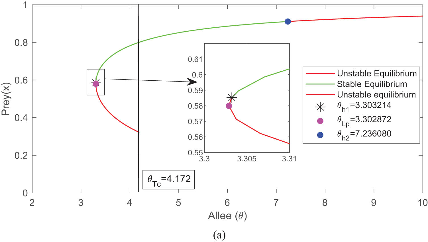
This is the one parametric bifurcation diagram, where the Allee considered as a bifurcations parameter. This diagram shows that Hopf bifurcations are occurs at
6 Numerical simulation
In this section, we describe the dynamics of model (4) numerically, for which we have used the mathematical tools Matlab and Maple. The Runge-Kutta fourth order method is used to describe the dynamical behaviour of the model. The analytical and numerical studies give exactly the same results, which means that the study of dynamical behaviour like equilibria and their stability, as well as some local bifurcations, in both analytical and numerical studies gives the same results for the valid set of parameters. We have fixed the parameters set (1) for further numerical simulation.
In order to conduct more numerical simulations, we maintain the fixed parameters and investigate the impact of the Allee parameter by varying its value. This part focuses on the examination of the dynamical properties, including stability and bifurcation, of the model with respect to its equilibrium points. By using the Maple software (mathematical tool), we have verified the analytical results numerically. Now we have plotted one-dimensional bifurcation diagram using the bifurcation parameter Allee
To study a Hopf bifurcation point more closely, you can indeed plot various visual representations of the system’s behaviour, including phase portrait, limit cycle, and time series. A limit cycle is a closed trajectory in the phase space, representing the oscillatory behaviour. This can help you visualise the system’s periodic motion. The time series plots show how the system’s behaviour evolves over time and can illustrate the transition to oscillatory behaviour at the Hopf bifurcation point. This article investigates bifurcation diagrams, limit cycles, and time series plots in the next subsections.
6.1 Bifurcation diagram
Figure 2 describes two interior equilibria for
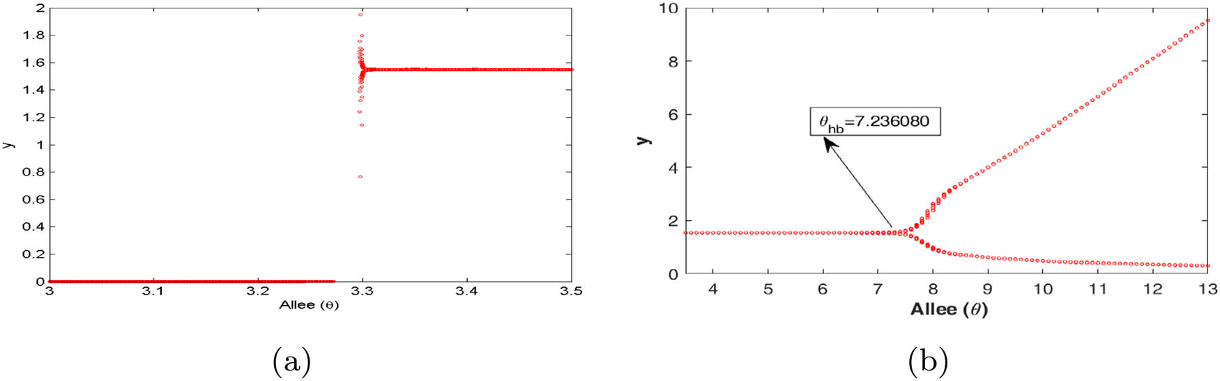
(a and b) Bifurcation diagrams with
6.2 Limit cycle and time series at Hopf bifurcation points
Figures 4, 5, 6 are drawn for the fixed parameters set (A) given in Table 1 and the Hopf bifurcation points
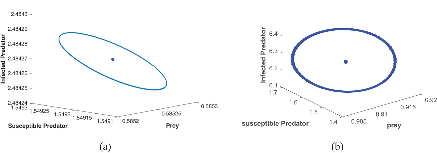
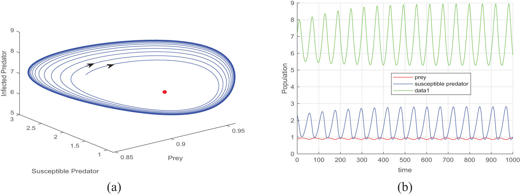
(a) Limit cycle at Hopf point
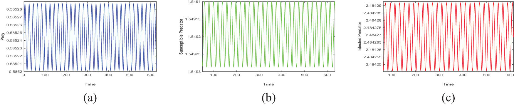
The figures (a), (b), and (c) are time series plots that ensure periodic oscillation of the model (4) at Hopf point
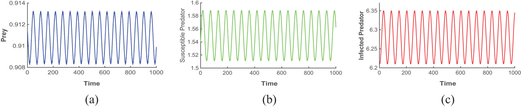
The figures (a), (b), and (c) are time series plots that ensure periodic oscillation of the model (4) at Hopf point
Figures 4, 5, and 6 depict the periodic oscillations of model (4). This periodic oscillation suggests that the species in the ecosystem exhibit cyclic fluctuations, indicating that their populations are not permanently stable and do not face immediate extinction. Instead, these oscillations imply that the species remains in existence over time despite the recurrent population fluctuations. Hence, we can say from the figure that all the species of prey, susceptible predator, and infected predator exist in the form of recurrent population fluctuations.
6.3 Phase portrait in the different region of the Allee parameter
The phase portraits are plotted for the different region of the Allee parameter, and the all other parameters are the same as fixed. Figure 2 shows three Allee parameter region
In Figure 7, it is depicted that after passing the second Hopf bifurcation point, marked as
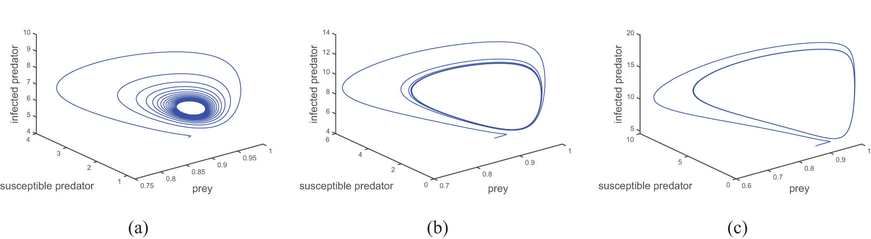
This figure shows the limit cycle behaviour after Hopf bifurcation point

(a) The phase portrait indicates that there are two interior equilibria, one of which is stable and the other is unstable. Furthermore, it demonstrates that the trivial equilibrium is stable when
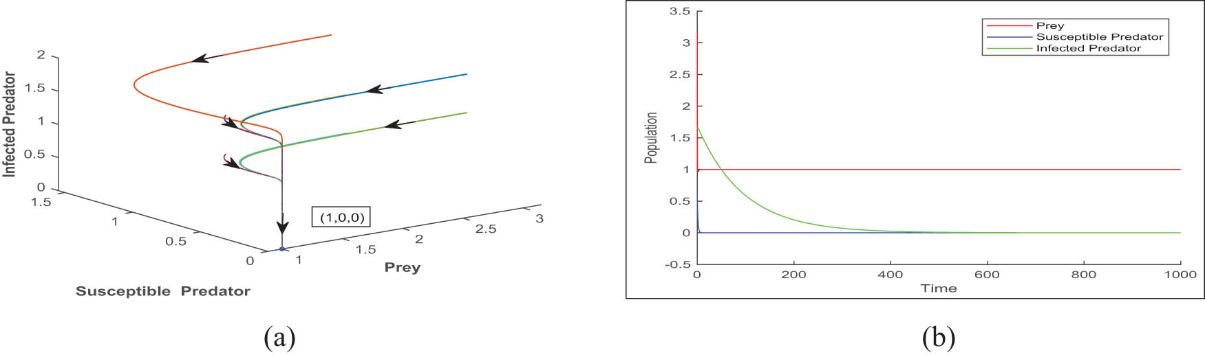
(a) A phase portrait showing that the axial equilibrium
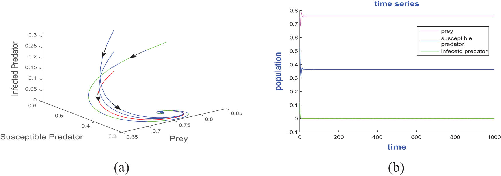
(a) A phase portrait showing that the disease-free equilibrium point

(a) A phase portrait for the Hopf threshold value
Now discuss the phase portrait about the axial and boundary equilibrium points for different sets of parameters mentioned in the caption of Figure 9 and 10, respectively.
(a) The stable limit cycle behaviour around the unstable equilibrium point, and (b) the periodic oscillation for the same. Taken
7 Discussion and conclusions
The Allee effect has huge impact on the eco-epidemiological model and also gives a good understanding of ecology and epidemiological issues. This article investigated all possible biologically feasible steady states of model (4) and also studied the stability of model (4) for every feasible equilibrium state. The ability for all species to coexist in a stable or oscillatory manner is dependent upon a set of parametric restrictions, with the Allee effect playing a significant part throughout the system. The Allee effect can destabilise the system; see the bifurcation diagram 2. The stability of the model about the interior equilibrium points switches, and the system appeared to be Hopf bifurcation, where the Allee effect plays an important role as a bifurcation parameter (Figure 2). The asymptotic stability of the system was examined for all possible equilibrium states. The investigation has been conducted on the presence of Hopf bifurcation in nearby areas of both the disease-free and interior equilibrium states. Figures 5 and 6 shows that all species exist together in oscillatory motion in presence of the Allee effect and diseases. All the species (prey, susceptible predator, and infected predator) co-exists and stable together for the Allee parameter
Acknowledgments
The authors express their gratitude to the reviewers for their valuable comments and suggestions. Additionally, appreciation is extended to the editor for their insightful input. The authors would like to thank their friends Saddam Hussain and Amit Kumar for their indispensable assistance throughout the preparation of this paper.
-
Funding information: This research received no specific grant from any funding agency and commercial or nonprofit sectors.
-
Author contributions: Bipin Kumar conceived the idea, conducted analyses and simulations, and drafted the manuscript. Rajesh kumar Sinha conceptualized the flow for the entire draft of the manuscript, verified all the results and edited the draft.
-
Conflict of interest: The authors declare that they have no conflict of interest.
-
Ethical approval: This research did not require any ethical approval.
-
Informed consent: Informed consent has been obtained from all individuals included in this study.
-
Data availability statement: Data sharing is not applicable to this article as no new data were created or analyzed in this study.
References
[1] Ali, N., Haque, M., Venturino, E., & Chakravarty, S. (2017). Dynamics of a three species ratio-dependent food chain model with intra-specific competition within the top predator. Computers in Biology and Medicine, 85, 63–74. 10.1016/j.compbiomed.2017.04.007Search in Google Scholar PubMed
[2] Allee, W. C. (1927). Animal aggregations. The Quarterly Review of Biology, 2(3), 367–398. 10.1086/394281Search in Google Scholar
[3] Anderson, R., Medley, G., May, R., & Johnson, A. (1986). A preliminary study of the transmission dynamics of the human immunodeficiency virus (HIV), the causative agent of aids. Mathematical Medicine and Biology: A Journal of the IMA, 3(4), 229–263. 10.1093/imammb/3.4.229Search in Google Scholar PubMed
[4] Anderson, R. M., Heesterbeek, H., Klinkenberg, D., & Hollingsworth, T. D. (2020). How will country-based mitigation measures influence the course of the covid-19 epidemic? The Lancet, 395(10228), 931–934. 10.1016/S0140-6736(20)30567-5Search in Google Scholar PubMed PubMed Central
[5] Angulo, E., Roemer, G. W., Berec, L., Gascoigne, J., & Courchamp, F. (2007). Double Allee effects and extinction in the island fox. Conservation Biology, 21(4), 1082–1091. 10.1111/j.1523-1739.2007.00721.xSearch in Google Scholar PubMed
[6] Arancibia-Ibarra, C., & Flores, J. (2021). Dynamics of a Leslie-Gower predator-prey model with Holling type ii functional response, Allee effect and a generalist predator. Mathematics and Computers in Simulation, 188, 1–22. 10.1016/j.matcom.2021.03.035Search in Google Scholar
[7] Arditi, R., & Ginzburg, L. R. (2012). How species interact: altering the standard view on trophic ecology. Oxford University Press. 10.1093/acprof:osobl/9780199913831.001.0001Search in Google Scholar
[8] Birkhoff, G., & Rota, G. (1982). Ordinary differential equation, Boston: Ginn. and co. Search in Google Scholar
[9] Brauer, F., Castillo-Chavez, C., & Castillo-Chavez, C. (2012). Mathematical models in population biology and epidemiology (Vol 2). Springer. 10.1007/978-1-4614-1686-9Search in Google Scholar
[10] Brearley, G., Rhodes, J., Bradley, A., Baxter, G., Seabrook, L., Lunney, D., …, McAlpine, C. (2013). Wildlife disease prevalence in human-modified landscapes. Biological Reviews, 88(2), 427–442. 10.1111/brv.12009Search in Google Scholar PubMed
[11] Chattopadhyay, J., & Arino, O. (1999). A predator-prey model with disease in the prey. Nonlinear Analysis, 36, 747–766. 10.1016/S0362-546X(98)00126-6Search in Google Scholar
[12] Courchamp, F., Clutton-Brock, T., & Grenfell, B. (2000). Multipack dynamics and the Allee effect in the African wild dog, Lycaon pictus. In Animal Conservation Forum (Vol. 3, pp. 277–285). Cambridge University Press. 10.1017/S1367943000001001Search in Google Scholar
[13] Das, K. P. (2016a). Complex dynamics and its stabilization in an eco-epidemiological model with alternative food. Modeling Earth Systems and Environment, 2(4), 1–12. 10.1007/s40808-016-0224-5Search in Google Scholar
[14] Das, K. P. (2016b). Disease-induced chaotic oscillations and its possible control in a predator-prey system with disease in predator. Differential Equations and Dynamical Systems, 24(2), 215–230. 10.1007/s12591-015-0249-7Search in Google Scholar
[15] Drake, J. M., & Kramer, A. M. (2011). Allee effects. Nature Education Knowledge, 3(10), 2. Search in Google Scholar
[16] Ghanbari, B. (2021). On the modeling of an eco-epidemiological model using a new fractional operator. Results in Physics, 21, 103799. 10.1016/j.rinp.2020.103799Search in Google Scholar
[17] Hadeler, K., & Freedman, H. (1989). Predator-prey populations with parasitic infection. Journal of Mathematical Biology, 27(6), 609–631. 10.1007/BF00276947Search in Google Scholar PubMed
[18] Hale, J. K. (1971). Functional differential equations. In Analytic theory of differential equations (pp. 9–22). Springer. 10.1007/BFb0060406Search in Google Scholar
[19] Hastings, A., & Powell, T. (1991). Chaos in a three-species food chain. Ecology, 72(3), 896–903. 10.2307/1940591Search in Google Scholar
[20] Kumar, U., Mandal, P. S., & Venturino, E. (2020). Impact of Allee effect on an eco-epidemiological system. Ecological Complexity, 42, 100828. 10.1016/j.ecocom.2020.100828Search in Google Scholar
[21] Kumar, V., & Kumari, N. (2021). Bifurcation study and pattern formation analysis of a tritrophic food chain model with group defense and Ivlev-like nonmonotonic functional response. Chaos, Solitons & Fractals, 147, 110964. 10.1016/j.chaos.2021.110964Search in Google Scholar
[22] Mandal, S., Al Basir, F., & Ray, S. (2021). Additive Allee effect of top predator in a mathematical model of three species food chain. Energy, Ecology and Environment, 6(5), 451–461. 10.1007/s40974-020-00200-3Search in Google Scholar
[23] Mccann, K., & Yodzis, P. (1995). Bifurcation structure of a three-species food-chain model. Theoretical Population Biology, 48(2), 93–125. 10.1006/tpbi.1995.1023Search in Google Scholar
[24] Mohammadi, H., Kumar, S., Rezapour, S., & Etemad, S. (2021). A theoretical study of the Caputo-Fabrizio fractional modeling for hearing loss due to mumps virus with optimal control. Chaos, Solitons & Fractals, 144, 110668. 10.1016/j.chaos.2021.110668Search in Google Scholar
[25] Mukherjee, D. (2010). Hopf bifurcation in an eco-epidemic model. Applied Mathematics and Computation, 217(5), 2118–2124. 10.1016/j.amc.2010.07.010Search in Google Scholar
[26] Mukhopadhyay, B., & Bhattacharyya, R. (2005). Dynamics of a delay-diffusion prey-predator model with disease in the prey. Journal of Applied Mathematics and Computing, 17(1), 361–377. 10.1007/BF02936062Search in Google Scholar
[27] Murray, J., & Seward, W. (1992). On the spatial spread of rabies among foxes with immunity. Journal of Theoretical Biology, 156(3), 327–348. 10.1016/S0022-5193(05)80679-4Search in Google Scholar
[28] Saenz, R. A., Hethcote, H. W., & Gray, G. C. (2006). Confined animal feeding operations as amplifiers of influenza. Vector-Borne & Zoonotic Diseases, 6(4), 338–346. 10.1089/vbz.2006.6.338Search in Google Scholar PubMed PubMed Central
[29] Sahoo, B., & Poria, S. (2014). Diseased prey predator model with general Holling type interactions. Applied Mathematics and Computation, 226, 83–100. 10.1016/j.amc.2013.10.013Search in Google Scholar PubMed PubMed Central
[30] Sarangi, B., & Raw, S. (2023). Dynamics of a spatially explicit eco-epidemic model with double Allee effect. Mathematics and Computers in Simulation, 206, 241–263. 10.1016/j.matcom.2022.11.004Search in Google Scholar
[31] Sen, M., Banerjee, M., & Morozov, A. (2015). A generalist predator regulating spread of a wildlife disease: Exploring two infection transmission scenarios. Mathematical Modelling of Natural Phenomena, 10(2), 74–95. 10.1051/mmnp/201510206Search in Google Scholar
[32] Shaikh, A. A., & Das, H. (2020). An eco-epidemic predator-prey model with Allee effect in prey. International Journal of Bifurcation and Chaos, 30(13), 2050194. 10.1142/S0218127420501941Search in Google Scholar
[33] Skalski, G. T., & Gilliam, J. F. (2001). Functional responses with predator interference: Viable alternatives to the Holling type ii model. Ecology, 82(11), 3083–3092. 10.1890/0012-9658(2001)082[3083:FRWPIV]2.0.CO;2Search in Google Scholar
[34] Stephens, P. A., Sutherland, W. J., & Freckleton, R. P. (1999). What is the Allee effect? Oikos, 185–190. 10.2307/3547011Search in Google Scholar
[35] Strogatz, S. H. (2018). Nonlinear dynamics and chaos: With applications to physics, biology, chemistry, and engineering. CRC Press. 10.1201/9780429399640Search in Google Scholar
[36] Vinoth, S., Sivasamy, R., Sathiyanathan, K., Rajchakit, G., Hammachukiattikul, P., Vadivel, R., & Gunasekaran, N. (2021). Dynamical analysis of a delayed food chain model with additive Allee effect. Advances in Difference Equations, 2021(1), 1–20. 10.1186/s13662-021-03216-zSearch in Google Scholar
[37] Wangersky, P. J. (1978). Lotka-Volterra population models. Annual Review of Ecology and Systematics, 9, 189–218. 10.1146/annurev.es.09.110178.001201Search in Google Scholar
[38] Wiggins, S., Wiggins, S., & Golubitsky, M. (2003). Introduction to applied nonlinear dynamical systems and chaos (Vol 2). Springer. Search in Google Scholar
[39] Yadav, R., Mukherjee, N., & Sen, M. (2022). Spatiotemporal dynamics of a prey-predator model with Allee effect in prey and hunting cooperation in a Holling type iii functional response. Nonlinear Dynamics, 107, 1397–1410. 10.1007/s11071-021-07066-ySearch in Google Scholar
© 2023 the author(s), published by De Gruyter
This work is licensed under the Creative Commons Attribution 4.0 International License.
Articles in the same Issue
- Special Issue: Infectious Disease Modeling In the Era of Post COVID-19
- A comprehensive and detailed within-host modeling study involving crucial biomarkers and optimal drug regimen for type I Lepra reaction: A deterministic approach
- Application of dynamic mode decomposition and compatible window-wise dynamic mode decomposition in deciphering COVID-19 dynamics of India
- Role of ecotourism in conserving forest biomass: A mathematical model
- Impact of cross border reverse migration in Delhi–UP region of India during COVID-19 lockdown
- Cost-effective optimal control analysis of a COVID-19 transmission model incorporating community awareness and waning immunity
- Evaluating early pandemic response through length-of-stay analysis of case logs and epidemiological modeling: A case study of Singapore in early 2020
- Special Issue: Application of differential equations to the biological systems
- An eco-epidemiological model with predator switching behavior
- A numerical method for MHD Stokes model with applications in blood flow
- Dynamics of an eco-epidemic model with Allee effect in prey and disease in predator
- Optimal lock-down intensity: A stochastic pandemic control approach of path integral
- Bifurcation analysis of HIV infection model with cell-to-cell transmission and non-cytolytic cure
- Special Issue: Differential Equations and Control Problems - Part I
- Study of nanolayer on red blood cells as drug carrier in an artery with stenosis
- Influence of incubation delays on COVID-19 transmission in diabetic and non-diabetic populations – an endemic prevalence case
- Complex dynamics of a four-species food-web model: An analysis through Beddington-DeAngelis functional response in the presence of additional food
- A study of qualitative correlations between crucial bio-markers and the optimal drug regimen of Type I lepra reaction: A deterministic approach
- Regular Articles
- Stochastic optimal and time-optimal control studies for additional food provided prey–predator systems involving Holling type III functional response
- Stability analysis of an SIR model with alert class modified saturated incidence rate and Holling functional type-II treatment
- An SEIR model with modified saturated incidence rate and Holling type II treatment function
- Dynamic analysis of delayed vaccination process along with impact of retrial queues
- A mathematical model to study the spread of COVID-19 and its control in India
- Within-host models of dengue virus transmission with immune response
- A mathematical analysis of the impact of maternally derived immunity and double-dose vaccination on the spread and control of measles
- Influence of distinct social contexts of long-term care facilities on the dynamics of spread of COVID-19 under predefine epidemiological scenarios