A comprehensive and detailed within-host modeling study involving crucial biomarkers and optimal drug regimen for type I Lepra reaction: A deterministic approach

Dinesh Nayak; Bishal Chhetri; Krishna Kiran Vamsi Dasu; Swapna Muthusamy; Vijay M. Bhagat

doi:10.1515/cmb-2022-0148

Article Open Access

A comprehensive and detailed within-host modeling study involving crucial biomarkers and optimal drug regimen for type I Lepra reaction: A deterministic approach

Dinesh Nayak , Bishal Chhetri , Krishna Kiran Vamsi Dasu , Swapna Muthusamy and Vijay M. Bhagat

Published/Copyright: June 16, 2023

Published by

Become an author with De Gruyter Brill

Submit Manuscript Author Information

From the journal Computational and Mathematical Biophysics Volume 11 Issue 1

Abstract

Leprosy (Hansen’s disease) is an infectious, neglected tropical disease caused by the Mycobacterium Leprae (M. Leprae). About 2,02,189 new cases are diagnosed worldwide each year. Lepra reactions are an off shoot of leprosy infection causing major nerve damage leading to disability. Early detection of lepra reactions through the study of biomarkers can prevent subsequent disabilities. Motivated by these observations, in this study, we have proposed and analyzed a three-dimensional mathematical model to capture the dynamics of susceptible schwann cells, infected schwann cells, and the bacterial load based on the pathogenesis of leprosy. We did the stability analysis, numerical simulations, and also performed the sensitivity analysis using Spearman’s rank correlation coefficient, partial rank correlation coefficient, and Sobol’s index methods. We later performed the optimal control studies with both multi-drug therapy and steroid interventions as control variables. Finally, we did the comparative and effectiveness study of these different control interventions.

Keywords: Hansen’s disease; type I lepra reaction; PRCC method; SRCC method; Sobol’s index; MDT; comparative and effectiveness study

MSC 2010: 37Nxx; 92BXX; 92Cxx

1 Introduction

Leprosy is an infection caused by slow-growing bacteria called Mycobacterium leprae. Leprosy is also known as Hansen disease, and it is considered to be the oldest disease known to humans. Primarily the bacteria affects the skin and peripheral nerves of the host body. In some of the cases, it affects the mucosa of the upper respiratory tract and the eyes. According to the WHO report [25], the global annual number of new cases detected in 2019 was about 2,02,189. In 2017, more than half million people were disabled due to leprosy, and almost 50,000 are added every year worldwide. Specifically in the Indian scenario as on March 2021, 79,898 patients were under free multi drug therapy (MDT) treatment for leprosy in which 65,147 were new cases [39]. In leprosy, lepra reactions are the major cause for nerve damage leading to disability. Early detection of lepra reactions through the study of biomarkers have important role in prevention of subsequent disabilities.

During the course of the leprosy disease, there can be sudden changes in immune-mediated response to Mycobacterium leprae antigen, which are referred to as leprosy (lepra) reactions. The reactions manifest as acute inflammatory episodes rather than chronic infectious course. There are mainly two types of leprosy reactions. Type 1 reaction is associated with cellular immunity and particularly with the reaction of T helper 1 (Th1) cells to mycobacterial antigens. This reaction involves exacerbation of old lesions leading to the erythematous appearance. Type 2 reaction or erythema nodosum leprosum is associated with humoral immunity. It is characterized by systemic symptoms along with new erythematous subcutaneous nodules.

Several clinical and experimental studies have been done on leprosy. Some works deal about the growth of the M. Leprae [23], and some studies on pathogenesis [21]. Some mathematical modeling studies dealing with infectious disease can be found in [1,31,34,36]. Specifically in the context of the leprosy modeling, the work [5] explores the dynamics of transmission of leprosy at population level, and in [12], the transmission dynamics of the multibacillary leprosy, and paucibacillary leprosy including a delay is dealt with. In [11], the cellular level dynamics of leprosy are explored. To our knowledge as of date, there is no work done yet to explore the dynamics at the level of biomarkers for leprosy, and also there seems to be no mathematical literature available dealing with the optimal drug regimen for treating leprosy and lepra reactions. A mathematical modeling study to this extent will help the clinicians to dissemination of the leprosy by targeting the crucial biomarkers with minimal damage and also helps them for the optimal drug regimen.

Motivated by the aforementioned observations, in this study, we have proposed and analyzed an within-host three-dimensional mathematical model to capture the dynamics of susceptible schwann cells, infected schwann cells, and the bacterial load involving the causation biomarkers for type I lepra reaction based on a detailed flowchart dealing with the pathogenesis of leprosy developed from the clinical works [28,30,38] and depicted in Figure 1. We initially study the natural history of the disease followed by studies on the optimal drug regimen for type I lepra reaction.

Figure 1

Frame (a) depicts the flow chart of the Pathogenesis of leprosy in side human body in brief. Frame (b) depicts the flow chart of the Pathogenesis of leprosy in side human body in detail.

This article is organized as follows. In Section 2, we formulate the mathematical model dealing with the type I lepra reaction based on its pathogenesis. In Section 3, we establish the existence, positivity, and boundedness of the developed model followed by the local and global stability of different equilibria about the reproduction number value ℛ 0 = 1 followed by the bifurcation analysis. Further, in Section 4, we numerically depict the theoretical findings of Section 3. We validate the proposed model via the leprosy disease characteristics using 2D heat plots in Section 5. In Section 6, we perform the sensitivity analysis of the model parameters. Later in Section 7, we do the optimal control studies considering the different medication involved in the MDT as control variables followed by optimal control studies involving both MDT and steroid interventions. We do the comparative and effectiveness study of these different control interventions in Section 8 followed by the discussions and conclusions in Section 9.

2 Mathematical model formulation

On the basis of the pathogenesis of leprosy dealt in the flowchart in Figure 1, we consider a three-compartment model dealing with susceptible schwann cells S ( t ) , infected schwann cells I ( t ) , and the bacterial load B ( t ) . We have taken the help of system of ODEs to interpret the biological dynamics in terms of mathematical equations.

The dynamics of the susceptible cells, i.e., d S d t will depend on the natural birth rate ω . Also according to the law of mass action, the susceptible cells decrease at a rate β and hence the term − β S B . The susceptible cells decrease due to the natural death and the cytokines responses. Next for the dynamics of the infected cells, i.e., d I d t , the infected cells increase by β S B and decrease by the natural death and cytokines responses. There is an indirect increase in the growth of the bacteria owing to the burst rate of the infected cells as more bacteria are now freely available to infect the susceptible schwann cells. Therefore, the compartment d B d t has α I , and the bacterial load decreases due to natural death of the bacteria and death due to the cytokines. In summary, we propose the following within-host model dealing with type I lepra reaction through TH-1 pathway.

(1) d S d t = ω − β S B − γ S − μ 1 S ,

(2) d I d t = β S B − δ I − μ 1 I ,

(3) d B d t = α I − ( d 11 + d 12 + d 13 + d 14 + d 15 + d 16 + d 17 ) B − μ 2 B ,

Symbols	Biological meaning
S	Susceptible schwann cells
I	Infected schwann cells
B	Bacterial load
ω	Natural birth rate of the susceptible cells
β	Rate at which schwann cells are infected
γ	Death rate of the susceptible cells due to cytokines
μ 1	Natural death rate of schwann cells and infected schwann cells
δ	Death rate of infected schwann cells due to cytokines
α	Burst rate of infected schwann cells realizing the bacteria
d 11 , d 12 , d 13 , d 14 , d 15 , d 16 , d 17	Rates at which M. Leprae is removed because of the release of cytokines IL-2, IL-7, TNF - α , IFN - γ , IL-12, IL-15, IL-17, respectively
μ 2	Natural death rate of M. Leprae

3 Stability analysis

3.1 Positivity and boundedness

Theorem 1

(Positivity) For the model (1)–(3) if initially S ( 0 ) > 0 , I ( 0 ) > 0 , and B ( 0 ) > 0 then for all t ∈ [ 0 , t 0 ] , where t 0 > 0 , S ( t ) , I ( t ) , and B ( t ) will remain positive in R + 3 .

Proof

We now aim to show that for all t ∈ [ 0 , t 0 ] , S ( t ) , I ( t ) , and B ( t ) will be positive in R + 3 .

Consider

d S d t = ω − β S B − γ S − μ 1 S ≥ − ( β B + γ + μ 1 ) S .

On solving the aforementioned inequality, we obtain

S ( t ) ≥ e − ( γ t + μ 1 t + ∫ B d t ) > 0

∴ S ( t ) > 0 , ∀ t ∈ [ 0 , t 0 ] .

In similar lines, we see that

d I d t ≥ − δ I − μ 1 I ⇒ I ( t ) ≥ e − ( δ + μ 1 ) t > 0 d B d t ≥ − y B − μ 2 B ⇒ B ( t ) ≥ e − ( y + μ 2 ) t > 0 .

Here, we let y = ( d 11 + d 12 + d 13 + d 14 + d 15 + d 16 + d 17 ) . Thus, for all t ∈ [ 0 , t 0 ] , S ( t ) , I ( t ) , and B ( t ) will remain positive, i.e., in R + 3 .□

Theorem 2

(Boundedness) There exists an upper bound for each of the variable S ( t ) , I ( t ) , and B ( t ) for all t ∈ [ 0 , t 0 ] .

Proof

Let us consider

d S d t + d I d t = ω − ( γ + μ 1 ) S − ( δ + μ 1 ) I ⇒ d ( S + I ) d t ≤ ω − min { ( γ + μ 1 ) , ( δ + μ 1 ) } ( S + I ) .

Considering k = min { ( γ + μ 1 ) , ( δ + μ 1 ) } and integrating the aforementioned equation, we obtain

( S + I ) ( t ) ≤ ω k + c 1 e − k t .

Hence,

limsup t → ∞ ( S + I ) ≤ limsup t → ∞ ω k + c 1 e − k t = ω k < ∞ .

∴ ( S + I ) ( t ) is bounded, and thus, S ( t ) , I ( t ) are bounded. Hence,

S ( t ) , I ( t ) ≤ ( S + I ) ( t ) .

Now for t ∈ [ 0 , t 0 ] , there exist S max and I max such that S ( t ) ≤ S max , I ( t ) ≤ I max .

We now consider d B d t = α I − ( y + μ 2 ) B .

Solving the aforementioned differential equation for B ( t ) , we obtain

B e ( y + μ 2 ) t = ∫ α I e ( y + μ 2 ) t d t ≤ ∫ α ω k e ( y + μ 2 ) t d t = α ω k ( y + μ 2 ) e ( y + μ 2 ) t + c 2 ⇒ B ( t ) ≤ α ω k ( y + μ 2 ) + c 2 e − ( y + μ 2 ) t

∴ limsup t → ∞ B ( t ) ≤ limsup t → ∞ α ω k ( y + μ 2 ) + c 2 e − ( y + μ 2 ) t = α ω k ( y + μ 2 ) < ∞ .

Hence, there exists an upper bound for B ( t ) , say B max for t ∈ [ 0 , t 0 ] .

Hence, S ( t ) , I ( t ) and B ( t ) all are bounded for t ∈ [ 0 , t 0 ] . □

3.2 Existence of the solution

Theorem 3

Let t 0 > 0 . If the model (1)–(3) initially satisfy S ( 0 ) > 0 , I ( 0 ) > 0 and B ( 0 ) > 0 , then ∀ t > 0 and there exists a unique solution for the system in R + 3 .

Proof

The system (1)–(3) in the vectorial form are given by

d X d t = f ( X ) ,

where

X = S ( t ) I ( t ) B ( t ) and f ( X ) = ω − β S B − γ S − μ 1 S β S B − δ I − μ 1 I α I − y B − μ 2 B .

Now we can see that f ( X ) : R 3 → R 3 has a continuous derivative, and thus, it is locally lipschitz in R 3 . Hence, from fundamental existence and uniqueness theorem [2, 33], we can conclude the existence of unique solution for the system (1)–(3).□

3.3 Equilibrium points and the reproduction number ℛ 0

The basic reproduction number for the system (1)–(3) is calculated using the next-generation matrix method [13], and the expression for ℛ 0 is found to be

ℛ 0 = α β ω ( γ + μ 1 ) ( δ + μ 1 ) ( y + μ 2 ) .

We also see that the system (1)–(3) admits two equilibria, namely, the infection/disease free equilibrium E 0 = ω μ 1 , 0 , 0 and the infected equilibrium E ∗ = ( S ∗ , I ∗ , B ∗ ) , where

S ∗ = ( δ + μ 1 ) ( y + μ 2 ) α β = ω ( γ + μ 1 ) ℛ 0 I ∗ = α β ω − ( γ + μ 1 ) ( δ + μ 1 ) ( y + μ 2 ) α β ( δ + μ 1 ) = ( γ + μ 1 ) ( y + μ 2 ) ( ℛ 0 − 1 ) α β B ∗ = α β ω − ( γ + μ 1 ) ( δ + μ 1 ) ( y + μ 2 ) β ( δ + μ 1 ) ( y + μ 2 ) = ( γ + μ 1 ) ( ℛ 0 − 1 ) β .

3.4 Stability analysis of E 0

3.4.1 Local stability

In the following, we do the local stability analysis of the infection free equilibrium E 0 .

The Jacobian matrix of the system at the infection free equilibrium E 0 is given by,

J E 0 = − ( γ + μ 1 ) 0 − β ω ( γ + μ 1 ) 0 − ( δ + μ 1 ) β ω ( γ + μ 1 ) 0 α − ( y + μ 2 )

The characteristic equation is given by

(4) ( − ( γ + μ 1 ) − λ ) λ 2 + { ( γ + μ 1 ) + ( y + μ 2 ) } λ + ( γ + μ 1 ) ( y + μ 2 ) − β α ω ( γ + μ 1 ) = 0 .

One of the eigenvalues of the aforementioned equation is λ 1 = − ( γ + μ 1 ) , which is less than zero, and the other two eigenvalues are calculated as follows:

Introducing ℛ 0 in the rest part of the equation:

(5) λ 2 + { ( γ + μ 1 ) + ( y + μ 2 ) } λ + ( γ + μ 1 ) ( y + μ 2 ) ( 1 − ℛ 0 ) = 0 .

Letting A = ( γ + μ 1 ) + ( y + μ 2 ) and D = ( γ + μ 1 ) ( y + μ 2 ) , the roots of the aforementioned equation are given by

λ = 1 2 [ − A ± A 2 + 4 ( ℛ 0 − 1 ) D ] .

We now consider the following two cases for understanding the stability of infection free equilibrium.

Case I: When ℛ 0 < 1

Further, in this case, we need to consider the following two sub cases:

A 2 + 4 ( ℛ 0 − 1 ) D > 0
A 2 + 4 ( ℛ 0 − 1 ) D < 0

Subcase (a): When A 2 + 4 ( ℛ 0 − 1 ) D > 0 , since the parameters are positive, which make D > 0 and 4 ( ℛ 0 − 1 ) D < 0 . Now considering k = 4 ( ℛ 0 − 1 ) D ,

A 2 + k < A 2 ⇒ A 2 + k < A .

This means A 2 + 4 ( ℛ 0 − 1 ) D < A always, then the eigenvalues are given by,

λ 2 , 3 = 1 2 [ − A ± A 2 + 4 ( ℛ 0 − 1 ) D ] ,

which are less than zero.

Therefore, the infection free equilibrium point E 0 is asymptotically stable in this case as all the eigenvalues are negative.

Subcase (b): When A 2 + 4 ( ℛ 0 − 1 ) D < 0 , the eigenvalues are complex conjugates with the negative real parts. Therefore, in this case also, we have E 0 to be asymptotically stable.

Hence, we conclude that E 0 is locally asymptotically stable whenever ℛ 0 < 1 .

Case II: When ℛ 0 > 1

In this case the characteristic equation has two negative eigenvalues and one positive eigenvalue. Hence, whenever ℛ 0 > 1 , the infection free equilibrium E 0 becomes unstable.

3.4.2 Global stability

As in Korobeinikov [16], we consider the Lyapunov function of the system (1)–(3) as follows:

U ( S , I , B ) = S 0 S S 0 − ln S S 0 + I + ( δ + μ 1 ) α B .

Now

d U d t = ω 2 − S S 0 − S 0 S + ( δ + μ 1 ) ( y + μ 2 ) α ( ℛ 0 − 1 ) B .

Here, 2 − S S 0 − S 0 S < 0 , and for ℛ 0 < 1 , the derivative d u d t < 0 .

∴ For ℛ 0 < 1 , the disease-free equilibrium E 0 is globally asymptotically stable (GAS).

3.5 Stability analysis of E ∗

3.5.1 Local stability

The Jacobian matrix of the system for E ∗ is given by

J = − ( γ + μ 1 ) ℛ 0 0 − ( δ + μ 1 ) ( y + μ 2 ) α ( γ + μ 1 ) ( ℛ 0 − 1 ) − ( δ + μ 1 ) ( δ + μ 1 ) ( y + μ 2 ) α 0 α − ( y + μ 2 ) .

The characteristic equation of the Jacobian J evaluated at E ∗ is given by,

λ 3 + ( p + ( γ + μ 1 ) ℛ 0 ) λ 2 + ( p ( γ + μ 1 ) ℛ 0 ) λ + q ( γ + μ 1 ) ( ℛ 0 − 1 ) = 0 ,

where p = ( γ + μ 1 ) ( y + μ 2 ) and q = ( γ + μ 1 ) ( y + μ 2 ) .

Since ℛ 0 > 1 , ( p + ( γ + μ 1 ) ℛ 0 ) > 0 , ( p ( γ + μ 1 ) ℛ 0 ) > 0 , and q μ 1 ( ℛ 0 − 1 ) > 0 . Therefore, now if we substitute λ = − λ in the aforementioned characteristic equation and use the Descarte’s rule of sign change, we see that all the roots of the aforementioned characteristic equation to be negative. Hence, we conclude that the infected equilibrium point E 1 exists and remains asymptotically stable whenever ℛ 0 > 1 .

3.5.2 Global stability

Consider the Lyapunov function of the system (1)–(3) for E ∗ as in [16]

U ∗ ( S , I , B ) = S ∗ S S ∗ − ln S S ∗ + I ∗ I I ∗ − ln I I ∗ + ( δ + μ 1 ) α B ∗ B B ∗ − ln B B ∗ .

We see that

d U ∗ d t = ( γ + μ 1 ) S ∗ 2 − S S ∗ − S ∗ S + ( δ + μ 1 ) I ∗ 3 − S ∗ S − S B I ∗ S ∗ B ∗ I − I B ∗ I ∗ B .

Now since arithmetic mean is greater than or equal to the geometric mean, the quantities

S S ∗ + S ∗ S − 2 ≥ 0 and S ∗ S + S B I ∗ S ∗ B ∗ I + I B ∗ I ∗ B − 3 ≥ 0

Therefore, the derivative d U ∗ d t ≤ 0 for all S , I , B > 0 , which establish the GAS of E ∗ for ℛ 0 > 1 .

3.6 Bifurcation analysis

We now use the method given by Buonomo in [7] to do the bifurcation analysis for the system (1)–(3).

Theorem 4

The system (1)–(3) undergoes a trans-critical bifurcation at ℛ 0 = 1 , and it is forward.

Proof

Let us consider x 1 = I , x 2 = B , x 3 = S and x = ( x 1 , x 2 , x 3 ) .

Now we consider

Infected _ class d x 1 d t = β x 2 x 3 − ( δ + μ 1 ) x 1 d x 2 d t = α x 1 − ( y + μ 2 ) x 2 Uninfected _ class d x 3 d t = ω − β x 2 x 3 − ( γ + μ 1 ) x 3

and also f ( x ) = ( f 1 , f 2 , f 3 ) = d x 1 d t , d x 2 d t , d x 3 d t . Hence, f ( x ) is twice differentiable function in R 3 .

Further, we can interpret each f i as follows:

f i ( x ) = ℱ i ( x ) − V i ( x ) , i = 1 , 2 , 3 ,

where V i = V i − − V i + with

ℱ i ≔ Appearance rate of new infection in ith compartment.
V i + ≔ Transfer rate of individuals into the ith compartment.
V i − ≔ Transfer rate of individuals out of the ith compartment.

Therefore,

ℱ 1 = β x 2 x 3 , V 1 + = 0 , V 1 − = ( δ + μ 1 ) x 1
ℱ 2 = α x 2 , V 2 + = 0 , V 2 − = ( y + μ 2 ) x 2
ℱ 3 = 0 , V 3 + = 0 , V 3 − = β x 2 x 3 + ( γ + μ 1 ) x 3

Denoting X s as the set of all disease-free state, we have

X s ≔ { x ∈ R 3 : x 1 = 0 , x 2 = 0 } = 0 , 0 , ω ( γ + μ 1 ) .

Now we will satisfy the conditions A1–A5 of [7] as follows:

A1: All ℱ i , V i + and V i − are positive for i = 1 , 2 , 3 in the nonnegative cone { x ∈ R : x i ≥ 0 , i = 1 , 2 , 3 }

A2: If x ∈ X s , then V i − = 0 for the infected compartment, i.e., i = 1 , 2 . Since for x ∈ X s we have x 1 = 0 and x 2 = 0 ,

⇒ V 1 − = ( δ + μ 1 ) . 0 = 0 , V 2 − = ( y + μ 2 ) . 0 = 0 .

A3: No incidence of infection in uninfected compartment( x 3 ), i.e., ℱ 3 = 0

A4: Disease free subspace is invariant, that means for x ∈ X s , here ℱ i = 0 , V i + = 0 , i = 1 , 2

A5: Now putting all ℱ i = 0 , we have

f ( x ) = ( − ( δ + μ 1 ) x 1 , − ( y + μ 2 ) x 2 , ω − β x 2 x 3 − ( γ + μ 1 ) x 3 ) .

Now the derivative matrix of f ( x ) is given by

D f ( x ) = − ( δ + μ 1 ) 0 0 0 − ( y + μ 2 ) 0 0 β x 3 − β x 2 − ( γ + μ 1 ) ⇒ D f ( x 0 ) = − ( δ + μ 1 ) 0 0 0 − ( y + μ 2 ) 0 0 − β ω ( γ + μ 1 ) − ( γ + μ 1 ) ,

where x 0 ∈ X s , and here, D f ( x 0 ) is a lower triangular matrix with all negative diagonal entries, and hence, all the eigen values illustrating that the disease-free equilibrium is stable in the absence of new infections.

We now show that the following hypothesis H1–H3 of [7] is also satisfied.

H1: The only nonlinear term present in infected compartment of the system is ℱ 1 = β x 2 x 3 .

H2: Let T ( x 2 , x 3 ) = β x 2 x 3

T ( k x 2 , x 3 ) = β k . x 2 x 3 = k . β x 2 x 3 = k . T ( x 2 , x 3 )
T ( x 2 , k x 3 ) = β x 2 . k x 3 = k . β x 2 x 3 = k . T ( x 2 , x 3 )
T ( x 2 + x 2 ′ , x 3 ) = β ( x 2 + x 2 ′ ) x 3 = β x 2 x 3 + β x 2 ′ x 3 = T ( x 2 , x 3 ) + T ( x 2 ′ , x 3 )
T ( x 2 , x 3 + x 3 ′ ) = β x 2 ( x 3 + x 3 ′ ) = β x 2 x 3 + β x 2 x 3 ′ = T ( x 2 , x 3 ) + T ( x 2 , x 3 ′ )

Therefore, the nonlinear term in the above hypothesis (H1) is bilinear in nature.

H3: There is no transfer from infected compartment to uninfected compartment.

Now by using Proposition 1 in [7], we can conclude that the system (1)–(3) undergoes a trans-critical bifurcation at ℛ 0 = 1 , which is forward in nature.□

4 Numerical simulations

All the values of the parameters used here are estimated from different clinical papers. The appropriate references are cited in the Table 1. For the parameters ω , μ 1 , and α , based on the doubling time available from the clinical literature, we have estimated the rate percentage using the formula rate % = log ( 2 ) doubling time ≈ 70 doubling time . We then divided the rate percentage by 100 to obtain the values/rates for these parameters. For estimating the parameters μ 1 , γ , and δ , we have taken the average of the rates in different medium such as 7-AAD, TUNNEL of the clinical experiments described in [24]. Some parameters are minimally fine tuned from Table 1 values to satisfy certain hypothesis/assumptions for convince of the numerical simulations.

Table 1

Values of the parameters complied from clinical literature

Symbols	Values	Units
ω	0.022 [15]	day − 1
β	3.44 [14]	day − 1
γ	0.1795 [24]	day − 1
μ 1	0.0018 [24]	day − 1
δ	0.2681 [24]	day − 1
α	0.063 [18]	day − 1
y	0.0003 [11]	day − 1
μ 2	0.57 [3]	day − 1

4.1 Disease free equilibrium E 0

We now depict the local and global stability of the disease-free equilibrium E 0 . Figure 2(a) and (b) depict the local and global stability of E 0 . For showing the local stability, we have chosen the initial value of the variables as S 0 = 520 , I 0 = 275 and B 0 = 250 , whereas for global stability, we considered different initial points.

$Figure 2 (a) The local stability at E 0 {E}_{0} from a single initial point. (b) The global stability at E 0 {E}_{0} starting from different initial points of the system (1)–(3).$

Figure 2

(a) The local stability at E 0 from a single initial point. (b) The global stability at E 0 starting from different initial points of the system (1)–(3).

We choose parameters in Table 2 and in such a way that ℛ 0 = 0.9939 < 1 , and for these parameters, we have E 0 = ( 55.1899 , 0 , 0 ) . For depicting the global stability of E 0 , we have arbitrarily considered the solution trajectories taking ten different initial conditions.

Table 2

Values of the parameters taken for E 0

ω	β	γ	μ 1	δ	α	y	μ 2
1.090	0.44	0.01795	0.0018	0.2681	0.0063	0.0003	0.57

4.2 Infected/endemic equilibrium E ∗

We now depict the local and global stability of the endemic equilibrium E ∗ . Figures 3(a) and (b) depict the local and global stability of E ∗ . The initial points are chosen in the similar way that we have chosen in case of E 0 .

$Figure 3 (a) Local stability at E ∗ {E}^{\ast } starting at a single initial point and (b) Global stability at E ∗ {E}^{\ast } starting from different initial points for the system (1)–(3).$

Figure 3

(a) Local stability at E ∗ starting at a single initial point and (b) Global stability at E ∗ starting from different initial points for the system (1)–(3).

For the numerical simulations, we have chosen the values of parameters as given in Table 3. For these parameter values, we have ℛ 0 = 29.6341 > 1 and the E ∗ = ( 38.9006 , 75.2748 , 17.3046 ) . For depicting the global stability of E ∗ , we have arbitrarily considered solution trajectories with different initial conditions.

Table 3

Values of the parameters taken for E ∗

ω	β	γ	μ 1	δ	α	y	μ 2
20.90	0.030	0.01795	0.00018	0.2681	00.2	0.3	0.57

4.3 Transcritical bifurcation

In this bifurcation, there is an exchange of stability between E 0 and E ∗ as ℛ 0 crosses unity. To depict this bifurcation, we varied the parameter ω from 0 to 0.25 with a step size of 0.001 and chose the other parameters from Table 1. Figure 4 depicts the occurrence of transcritical bifurcation at ℛ 0 = 1 .

$Figure 4 The transcritical bifurcation exhibited by the system (1)–(3) at ℛ 0 = 1 {{\mathcal{ {\mathcal R} }}}_{0}=1 .$

Figure 4

The transcritical bifurcation exhibited by the system (1)–(3) at ℛ 0 = 1 .

5 Model validation through 2D heat plots

From some of the clinical studies, we see that the average doubling time of the M. Leprae is approximately 14 days [27]. On the basis of this characteristic, we now validate the model (1)–(3) through the 2D heat plot.

We now vary the parameters α from 0.0563 to 0.0763 on the x -axis and the parameter γ between 0.15 and 0.2090 on the y -axis and generate a two-parameter heat plot to validate our model (1)–(3) by capturing the bacterial load ( B ) at 14th day. All other parameter are taken from Table 1, and the initial condition was chosen to be ( S 0 , I 0 , B 0 ) = ( 5,200 , 0 , 40 ) .

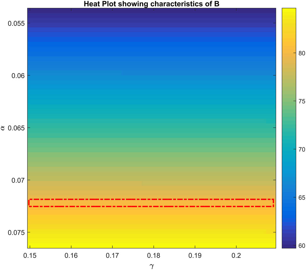
Now from Figure 5, it can be seen that the proposed model is able to reproduce characteristic, i.e., exactly the double of initial count of bacterial load, that is, 80 ( B 0 = 40 ), indicated by the dotted red rectangle.

Figure 5

Heat plot illustrating that the proposed model reproduces the clinical characteristics of leprosy. This can be seen from the red rectangular box, which the depicts the doubling value of the bacterial load (80) on the 14th day.

6 Sensitivity analysis

Here, we are interested in investigating the impact of uncertainty in the values of the different parameters on the variables ( S , I , B ). For this, we have used the global sensitivity analysis (GSA) methodology through Latin hyper cube sampling (LHS). LHS is a technique that involves sampling without the replacement a set of model parameter combinations from preset ranges on the parameter values [9,20,40]. Using this sample we generate the scatterplot to decide the methodology for GSA. The scatterplots enable the graphical detection of the nonlinearities, nonmonotonicities between model input (parameter) and output (variables). If the trend is nonlinear, then rank correlation coefficient such as partial rank correlation coefficient (PRCC), and Spearman’s rank correlation coefficient (SRCC) will be used for further sensitivity analysis where if the trend is nonmonotonic, the method based on the decomposition of model output variance such as Sobol’s method will be the best choice for further analysis. Since we want to study the impact of each parameter on each variable individually and also the cumulative effect of combination of parameters on each variable, we use both the SRCC and PRCC in our sensitivity analysis study.

6.1 LHS and Scatter plots

As an initial step to LHS, we select the following parameters listed in Table 4 having possible uncertainty in their values and consider them for the process of sampling. The range of the variable values used for sampling is listed in Table 4. All the parameter value ranges are chosen based on the clinical papers [18,24], and we introduced an uncertainty in y for our computational convenience. The remaining values of the parameters are as given in Table 1.

Table 4

Range of sensitive parameters

Parameter	Max value	Min value
γ	0.0763	0.0538
μ 1	0.0405	0.0305
δ	0.3099	0.2263
α	0.0763	0.0538
y	0.0001	0.0005

Then the LHS is done to create 1,000 sets of parameter sample each containing 5 random values of parameters. Now each set of these parameters was used to simulate the model at each time. Scatter plots were created for each parameter vs variable to decide the further procedure of GSA.

In Figure 6, we can easily see that the relationships between δ and all variables such as S ( t ) , I ( t ) , and B ( t ) follow a monotonic trend and the so is the case for y . Therefore, we did the SRCC and PRCC for these two variable, and the remaining parameters were analyzed by calculating the Sobol’s index.

$Figure 6 Scatter plots for parameters vs variables such as S ( t ) , I ( t ) S\left(t),I\left(t) , and B ( t ) B\left(t) .$

Figure 6

Scatter plots for parameters vs variables such as S ( t ) , I ( t ) , and B ( t ) .

6.2 SRCC and PRCC

By using the same sample obtained earlier, we calculated SRCC index separately for δ and y and the PRCC index jointly.

Figure 7 shows that δ has a more negative impact on S and I in comparison to y , whereas y has a more positive impact on B . The PRCC in Figure 8 shows that the cummulative impact of δ and y seems to be more on the infected cell population I .

$Figure 7 SRCC with respect to time, where δ \delta and y y are the input for each case of output variables S , I S,I , and B B .$

Figure 7

SRCC with respect to time, where δ and y are the input for each case of output variables S , I , and B .

$Figure 8 PRCC with respect to time. The combined impact of δ \delta and y y on S , I S,I , and B B .$

Figure 8

PRCC with respect to time. The combined impact of δ and y on S , I , and B .

6.3 Sobol’s index

The Sobol’s index is calculated using the formula of correlation [29].

S i = Corr ( Y , E ( Y ∕ x i ) ) ,

where S i is the Sobol’s index of ith parameter, Y is the model output value, and E ( Y ∕ x i ) is conditional expectation/mean of model output Y.

The Sobol’s index was calculated for the parameters μ 1 , γ , and α at each time as in SRCC and was plotted separately for the model variables S , I , and B , which can be seen in Figure 9. Unfortunately, from these figures, we could not derive any fruitful conclusions to decide the most sensitive parameter owing to the high fluctuations.

$Figure 9 Sobol’s index of μ 1 {\mu }_{1} , γ \gamma , and α \alpha with respect to S , I S,I , and B B is depicted in frames a, b and c respectively.$

Figure 9

Sobol’s index of μ 1 , γ , and α with respect to S , I , and B is depicted in frames a, b and c respectively.

Because of the aforementioned limitation, we tried to identify the sensitive parameters with respect to ℛ 0 , which is discussed in next section.

6.4 Sensitivity of ℛ 0

For identifying the sensitive parameters with respect to ℛ 0 , we did the scatterplots of the parameters against ℛ 0 and saw that none of them were qualified for PRCC analysis. Hence, we calculated the Sobol’s sensitivity index for each parameter and pairs of parameters as listed in frames of Figure 10.

$Figure 10 Frame (a) depicts sensitivity through Sobol’s Index with respect to ℛ 0 {{\mathcal{ {\mathcal R} }}}_{0} as output for model parameters individually. Frame (b) depicts sensitivity through Sobol's Index with respect to ℛ 0 {{\mathcal{ {\mathcal R} }}}_{0} as output for model parameters in combination of two.$

Figure 10

Frame (a) depicts sensitivity through Sobol’s Index with respect to ℛ 0 as output for model parameters individually. Frame (b) depicts sensitivity through Sobol's Index with respect to ℛ 0 as output for model parameters in combination of two.

6.5 Inference

From the aforementioned sensitivity analysis, we can conclude that α is the most sensitive parameter followed by δ and y . Here, α and δ have a direct impact on the system, where y has and inverse impact on the system as it has a negative Sobol’s index. In case of cumulative parameter sensitivity, we see that the parameter combination of α and δ is the most sensitive combination that impacts the system (1)–(3).

7 Optimal control studies

Currently, for type I lepra reaction, two kinds of medication are prescribed based on the disease condition [22,37]. First, MDT is used, and if still the reaction burden does not reduce, then steroids are given along with the MDT treatment.

Motivated by the aforementioned clinical findings, in this section, we frame and study two optimal control problems. First one deals with the optimal drug regimen for MDT and the second deals with the optimal drug regimen for the scenario involving both MDT and steroid interventions. These medical/drug interventions are modeled as control variables for the system (1)–(3).

7.1 Optimal control problem associated with MDT

According to the WHO recommended guidelines of 2018 for leprosy MDT consist of three drugs rifampin, dapsone, and clofazimine [22,35]. The drug rifampin acts as a rapid bacillary killer and thereby indirectly reduces the amount of cells getting infected. Therefore, the control variable D 12 ( t ) is negatively incorporated in the infected cell compartment of (7)–(9) and D 13 2 ( t ) is negatively incorporated in the bacterial load compartment of (7)–(9). Here, the square on D 13 ( t ) is used for capturing the extent of intense action of this drug on bacterial load. The drug dapsone is bactericidal and bacteriostatic against M. leprae [26]. To capture this action of the drug, we incorporate D 21 ( t ) and D 22 ( t ) in the compartments S and I of (7)–(9) and D 23 2 ( t ) in the B compartment of (7)–(9). The third drug clofazimine has an immuno-suppressive effect and also it binds with the DNA of the bacteria causing the inhibition of template function of DNA resulting bacteriostatic against M. leprae [10]. To incorporate this phenomenon, we add the control variable D 31 ( t ) to the S compartment in (7)–(9), resulting in increase of these cells. D 33 ( t ) is negatively incorporated in the B compartment of (7)–(9) to indicate the inhibition of bacterial replication.

Now mathematically we define the set of all control variables as follows:

U = { D i j ( t ) , D i j ( t ) ∈ [ 0 , D i j max ] , 1 ≤ i , j ≤ 3 , i j ≠ 32 , t ∈ [ 0 , T ] } .

Here, D i j max represents the maximum value of the corresponding control variable, which depends on the availability and limit of the drugs recommended for patients and T is the final time of observation.

Since the drugs in MDT can lead to some hazards, we consider a cost functional that minimizes the drug concentrations along with the infected cell count and bacterial load. On this basis, we define the following cost functional:

(6) J min ( D 1 , D 2 , D 3 ) = ∫ 0 T ( I ( t ) + B ( t ) + P [ D 11 2 ( t ) + D 12 2 ( t ) + D 13 3 ( t ) ] + Q [ D 21 2 ( t ) + D 22 2 ( t ) + D 23 3 ( t ) ] + R [ ∣ D 3 ( t ) ∣ 2 ] ) d t

subject to the constraints/system

(7) d S d t = ω − β S B − γ S − μ 1 S − D 11 ( t ) S − D 21 ( t ) S + D 31 ( t ) S

(8) d I d t = β S B − δ I − μ 1 I − D 12 ( t ) I − D 22 ( t ) I

(9) d B d t = ( α − D 23 2 ( t ) − D 33 ( t ) ) I − y B − μ 2 B − D 13 2 ( t ) B .

Here, D 1 = ( D 11 , D 12 , D 13 ) , D 2 = ( D 21 , D 22 , D 23 ) , D 3 = ( D 31 , D 33 ) , and ∣ • ∣ represents standard Euclidean norm in R n and ( D 1 , D 2 , D 3 ) ∈ U .

The integrand of the cost function (6), denoted by

(10) L ( I , B , D 1 , D 2 , D 3 ) = ( I ( t ) + B ( t ) + P [ D 11 2 ( t ) + D 12 2 ( t ) + D 13 3 ( t ) ] + Q [ D 21 2 ( t ) + D 22 2 ( t ) + D 23 3 ( t ) ] + R [ ∣ D 3 ∣ 2 ] ) ,

is the Lagrangian or running cost of the optimal control problem.

The admissible set of solutions for the aforementioned optimal control problem (6)–(9) is given by

Ω = { ( I , B , D 1 , D 2 , D 3 ) : I , B satisfying (7)–(9) ∀ ( D 1 , D 2 , D 3 ) ∈ U } .

7.2 Existence of optimal solution

In the section, we establish the existence of optimal control for the system (6)–(9) using the existence Theorem 2.2 of [6] dealing with nonlinear control systems.

Theorem 5

There exists a 8-tuple of optimal controls ( D 1 ∗ ( t ) , D 2 ∗ ( t ) , D 3 ∗ ( t ) ) in the set of admissible controls U such that the cost function is minimized, i.e.,

J ( D 1 ∗ ( t ) , D 2 ∗ ( t ) , D 3 ∗ ( t ) ) = min D 1 , D 2 , D 3 ∈ U { J ( D 1 , D 2 , D 3 ) }

corresponding to the control system (6)–(9), where D 1 = ( D 11 , D 12 , D 13 ) , D 2 = ( D 21 , D 22 , D 23 ) , D 3 = ( D 31 , D 33 ) .

Proof

Let us consider that d S d t = f 1 ( t , x , D ) , d I d t = f 2 ( t , x , D ) , and d B d t = f 3 ( t , x , D ) of the control system (6)–(9). Here, x ∈ X denotes the state variables ( S , I , B ) and D denote 8-tuple control variables. We take f = ( f 1 , f 2 , f 3 ) , then clearly X ⊂ R 3 and

f : [ 0 , T ] × X × U → R 3

is a continuous function of t and x for each D i j ∈ U . Now we have to show that ( F 1 )–( F 3 ) of Theorem 2.2 of [6] hold true.

F1: Here, each f i ’s have the continuous and bounded partial derivatives, which imply that the f is Lipschitz’s continuous.

F2: We consider g 1 ( D 11 , D 21 , D 31 ) = − D 11 − D 12 + D 31 , which is bounded on U . Thus,

f 1 ( t , x , D ( 1 ) ) − f 1 ( t , x , D ( 2 ) ) [ g 1 ( D ( 1 ) ) − g 1 ( D ( 2 ) ) ] = [ D 11 ( 2 ) + D 12 ( 2 ) − D 31 ( 2 ) − D 11 ( 1 ) − D 12 ( 1 ) + D 31 ( 1 ) ] S [ D 11 ( 2 ) + D 12 ( 2 ) − D 31 ( 2 ) − D 11 ( 1 ) − D 12 ( 1 ) + D 31 ( 1 ) ] ≤ η S = F 1 ( t , x ) ∴ f 1 ( t , x , D ( 1 ) ) − f 1 ( t , x , D ( 2 ) ) ≤ F 1 ( t , x ) • [ g 1 ( D ( 1 ) ) − g 1 ( D ( 2 ) ) ] .

Here, η > 1 is a real number. Moreover, since U compact and g 1 is continuous, we have g 1 ( U ) to be compact. Also since the function g 1 ( U ) is linear so the range of g 1 , i.e., g 1 ( U ) is will be convex. Since U is nonnegative so g 1 − 1 is nonnegative.

Similarly for f 2 ( t , x , D ) , we can choose g 2 ( D 12 , D 22 ) = − D 12 − D 22 and F 2 ( t , x ) = I and prove F2 in a similar way.

Now for f 3 ( t , x , D ) , we have to choose g 3 ( D 23 , D 33 ) = − D 23 2 − D 33

f 2 ( t , x , D ( 1 ) ) − f 2 ( t , x , D ( 2 ) ) [ g 2 ( D ( 1 ) ) − g 2 ( D ( 2 ) ) ] = [ D 23 2 ( 2 ) + D 33 ( 2 ) − D 23 2 ( 1 ) − D 33 ( 1 ) ] I − [ D 13 2 ( 1 ) − D 13 2 ( 2 ) ] B [ D 23 2 ( 2 ) + D 33 ( 2 ) − D 23 2 ( 1 ) − D 33 ( 1 ) ] ≤ [ D 23 2 ( 2 ) + D 33 ( 2 ) − D 23 2 ( 1 ) − D 33 ( 1 ) ] I [ D 23 2 ( 2 ) + D 33 ( 2 ) − D 23 2 ( 1 ) − D 33 ( 1 ) ] = I = F 3 ( t , x ) ( provided D 13 2 ( 1 ) ≥ D 13 2 ( 2 ) ) ∴ f 3 ( t , x , D ( 1 ) ) − f 3 ( t , x , D ( 2 ) ) ≤ F 3 ( t , x ) • [ g 3 ( D ( 1 ) ) − g 3 ( D ( 2 ) ) ] .

F3: Since S , I , B are bounded on [ 0 , T ] so F i ( • , x u ) ∈ ℒ 1 .

Now we have to show that the running cost function

C ( t , x , D ) = I ( t ) + B ( t ) + P [ D 11 2 ( t ) + D 12 2 ( t ) + D 13 3 ( t ) ] + Q [ D 21 2 ( t ) + D 22 2 ( t ) + D 23 3 ( t ) ] + R [ ∣ D 3 ( t ) ∣ 2 ]

satisfies the conditions ( C 1 ) − ( C 5 ) of Theorem 2.2 of [6]. Here, C : [ 0 , T ] × X × U → R

Here we see that C ( t , • , • ) is a continuous function as it is sum of continuous functions which are functions of t ∈ [ 0 , T ] .
Since S , I , and B and all D i j ’s are bounded implying that C ( • , x , D ) is bounded and hence measurable for each x ∈ X and D i j ∈ U .
Consider Ψ ( t ) = κ such that κ = min { I ( 0 ) , B ( 0 ) } , then Ψ will bounded such that for all t ∈ [ 0 , T ] , x ∈ X and D i j ∈ U , we have
C ( t , x , D ) ≥ Ψ ( t ) .
Since C ( t , x , D ) is sum of the function, which are convex in U for each fixed ( t , x ) ∈ [ 0 , T ] × X , therefore C ( t , x , D ) follows the same.
By using similar type of argument, we can easily show that for each fixed ( t , x ) ∈ [ 0 , T ] × X , C ( t , x , D ) is a monotonically increasing function.

Hence, we have shown that the optimal control problem satisfies all hypothesis of Theorem 2.2 of [6]. Therefore, there exists a 8- tuple of optimal controls ( D 1 ∗ ( t ) , D 2 ∗ ( t ) , D 3 ∗ ( t ) ) in the set of admissible controls U = { D i j ( t ) , D i j ( t ) ∈ [ 0 , D i j max ] , 1 ≤ i , j ≤ 3 , i j ≠ 32 , t ∈ [ 0 , T ] } such that the cost function is minimized.□

7.3 Characteristics for the optimal control

In this section, we obtain the characteristics of the optimal control using the Pontryagin’s maximum principle [19].

The Hamiltonian for the system (6)–(9) is given by

(11) H ( I , B , D 1 , D 2 , D 3 , λ ) = I ( t ) + B ( t ) + P [ D 11 2 ( t ) + D 12 2 ( t ) + D 13 3 ( t ) ] + Q [ D 21 2 ( t ) + D 22 2 ( t ) + D 23 3 ( t ) ] + R [ ∣ D 3 ( t ) ∣ 2 ] + λ 1 d S d t + λ 2 d I d t + λ 3 d B d t ,

where λ = ( λ 1 , λ 2 , λ 3 ) is the co-state vector or adjoint vector. Now the canonical equations that relates state variable and co-state variable are given by

(12) d λ 1 d t = − ∂ H ∂ S d λ 2 d t = − ∂ H ∂ I d λ 3 d t = − ∂ H ∂ B .

Now by substituting the value of the Hamiltonian into the aforementioned equation, we obtain

(13) d λ 1 d t = ( β B + μ 1 + γ + D 11 + D 21 − D 31 ) λ 1 − ( β B ) λ 2 d λ 2 d t = ( μ 1 + δ + D 12 + D 22 ) λ 2 − ( α − D 23 2 − D 33 ) λ 3 − 1 d λ 3 d t = ( β S ) λ 1 − ( β S ) λ 2 + ( y + μ 2 + D 13 2 ) λ 3 − 1

along with the transversality condition λ 1 ( T ) = 0 , λ 2 ( T ) = 0 , and λ 3 ( T ) = 0 . Now by using the fact that at optimal controls, D i j = D i j ∗ and the value of Hamiltonian is minimum implying that ∂ H ∂ D i j = 0 at D i j = D i j ∗ for 1 ≤ i , j ≤ 3 , and i j ≠ 32 , and by solving (7.7), we have the following values for the optimal controls.

D 11 ∗ = min max S λ 1 2 P , 0 , D 11 max D 12 ∗ = min max I λ 2 2 P , 0 , D 12 max D 13 ∗ = min max 2 I λ 3 3 P , 0 , D 13 max D 21 ∗ = min max S λ 1 2 Q , 0 , D 21 max D 22 ∗ = min max I λ 2 2 Q , 0 , D 22 max D 23 ∗ = min max 2 B λ 3 3 Q , 0 , D 23 max D 31 ∗ = min max − S λ 1 2 R , 0 , D 31 max D 33 ∗ = min max I λ 2 2 R , 0 , D 33 max .

7.4 Numerical studies for the optimal control problem with MDT

In this section, we numerically obtain the optimal drug regimen for the control problem (6)–(9) using the optimal controls obtained in the earlier section.

For the numerical simulations, we consider a time period of 100 days ( T = 100 ), and the parameter values are chosen as ω = 20.9 , β = 0.03 , μ 1 = 0.00018 , γ = 0.01795 , δ = 0.2681 , α = 0.2 , y = 0.3 , and μ 2 = 0.57 . First, we have solved the system numerically without any drug intervention. All the numerical calculations were done in MATLAB, and we used the 4th order Runge-Kutta method to solve the system of ODEs. Here, we consider the initial value of the state variables as S ( 0 ) = 520 , I ( 0 ) = 275 , and B ( 0 ) = 250 as in [11].

Further to simulate the system with controls, we use the forward–backward sweep method starting with the initial value of the controls as zero and estimate the sate variables forward in time. Since the transversality conditions have the value of adjoint vector at end time T , so the adjoint vector was calculated backward in time.

By using the value of state variables and adjoint vector, we calculate the control variables at each time instance that get updated in each iteration. We continue this till the convergence criterion is met [17].

The weights P , Q , and R in the cost function J min are chosen based on their hazard ratio of the corresponding drugs. We chose the weights directly proportional to the hazard ratios. In Table 5, the hazard ratios of the different drugs are enlisted. We have chosen the weights ( P , Q , and S ) proportional to the hazard ratios, i.e., P = 1 , Q = 1.99 , and R = 7.1 .

Table 5

Hazard ratio of the drugs

Drugs	Hazard ratio	Source
Rifampin	0.26	[4]
Dapsone	0.99	[8]
Clofazimine	1.85	[8]

We now numerically simulate the S , I , and B populations with single control intervention, with two control interventions and finally with all the three control interventions of MDT. In each of these figures, we also depict the no control intervention case for comparison purpose.

Figure 11 illustrates that when individually drugs are administered, the susceptible cell count decrease and the opposite effect is seen for infected cells and bacterial load compartments. From this figures we observe that the drug rifampin works the best in reducing the infected cells.

Figure 11

The dynamics of the S , I , and B populations when one drug is introduced.

Figure 12 depicts the combination of two-drug intervention case. As earlier, here also, we see the susceptible cell count increase with two-drug combination, and there is a decrease in both the infected cells and bacterial load compartments. From this figure, we observe that the drug combination of rifampin and dapsone works the best in reducing the infected cells and bacterial load.

Figure 12

The dynamics of the S , I , and B populations when combination of two drugs are introduced.

Figure 13 shows the dynamics of the S , I , and B populations with MDT intervention whose findings are in similar line to earlier two figures.

Figure 13

The dynamics of the S , I , and B populations with MDT intervention.

Table 6 gives the average S , I , and B cell count for single drug, two-drug combination, and MDT scenarios. From the table, it can be seen that MDT is the best and optimal combination for achieving the optimal increase in susceptible cells and optimal decrease in both infected cells and bacterial load.

Table 6

Average count of the S , I , and B cells for single drug, two-drug combination, and MDT scenarios

Drug combination	Avg susceptible cells	Avg infected cells	Avg bacterial load
Without drug	442.222583	351.081674	246.624000
Rifampin	455.500908	304.740187	168.887009
Dapsone	460.282734	311.553091	156.588949
Clofazimine	444.432478	350.135857	241.111031
Rifampin and dapsone	457.141441	286.714732	153.050429
Rifampin and clofazimine	454.385431	316.254129	181.777783
Dapsone and clofazimine	449.424133	307.980694	181.694639
MDT	457.899776	286.431294	150.360779

7.5 Optimal control problem associated with MDT along with steroids

Corticosteroid is a steroid that is mainly used for protecting the nerve damage by suppressing the cytokines responses caused due to the presence of M. leprae [32]. Also corticosteroid is usually given after the administration of MDT drugs owing to lepra reactions caused as a consequence of leprosy infection [32]. To capture this aspect and delay in administration of steroids, we introduce a time delay τ in the MDT control. In others words, we consider D ′ s at ( t − τ ) and consider the control associated with steroid as C ( t ) .

With the aforementioned modifications, the set of controls now is given by

U = { D i j ( t ) : D i j ( t ) ∈ [ 0 , D i j max ] , C ( t ) ∈ [ 0 , C max ] 1 ≤ i , j ≤ 3 , i j ≠ 32 , t ∈ [ 0 , T ] } ,

and the modified objective function and the control system are given by

(14) J min ( D 1 , D 2 , D 3 ) = ∫ 0 T ( I ( t ) + B ( t ) + P [ D 11 2 ( t − τ ) + D 12 2 ( t − τ ) + D 13 3 ( t − τ ) ] + Q [ D 21 2 ( t − τ ) + D 22 2 ( t − τ ) + D 23 3 ( t − τ ) ] + R [ ∣ D 3 ( t − τ ) ∣ 2 ] + T C 2 ( t ) ) d t ,

(15) d S d t = ω − β S B − γ S − μ 1 S − D 11 ( t − τ ) S − D 21 ( t − τ ) S + D 31 ( t − τ ) S + C ( t ) S ,

(16) d I d t = β S B − δ I − μ 1 I − D 12 ( t − τ ) I − D 22 ( t − τ ) I ,

(17) d B d t = ( α − D 23 2 ( t − τ ) − D 33 ( t − τ ) ) I − y B − μ 2 B − D 13 2 ( t − τ ) B .

Here, the Lagrangian is the integrand of the cost function (14) and is given by

(18) L ( I , B , D 1 , D 2 , D 3 , C ) = ( I ( t ) + B ( t ) + P [ D 11 2 ( t − τ ) + D 12 2 ( t − τ ) + D 13 3 ( t − τ ) ] + Q [ D 21 2 ( t − τ ) + D 22 2 ( t − τ ) + D 23 3 ( t − τ ) ] + R [ ∣ D 3 ( t − τ ) ∣ 2 ] + T C 2 ( t ) ) .

The admissible set of solutions for the aforementioned optimal control problem will now lie in the set

Ω = { ( I , B , D 1 , D 2 , D 3 , C ) : I , B satisfy (7)–(9) ∀ ( D 1 , D 2 , D 3 , C ) ∈ U } .

The existence of the optimal control can be shown in the similar way as it was shown in the previous optimal control problem in the preceding section.

We see that the Hamiltonian for the system (14)–(17) is given by

(19) H ( I , B , D 1 , D 2 , D 3 , λ ) = L ( I , B , D 1 , D 2 , D 3 , C ) + λ 1 d S d t + λ 2 d I d t + λ 3 d B d t ,

where λ = ( λ 1 , λ 2 , λ 3 ) is the co-state vector or adjoint vector. Now the canonical equations that relates state variable and co state variable are given by

(20) d λ 1 d t = − ∂ H ∂ S d λ 2 d t = − ∂ H ∂ I d λ 3 d t = − ∂ H ∂ B .

Now by substituting the value of the Hamiltonian in the aforementioned equation, we obtain

(21) d λ 1 d t = ( β B + μ 1 + γ + D 11 ( t − τ ) + D 21 ( t − τ ) − D 31 ( 1 − τ ) − C ( t ) ) λ 1 − ( β B ) λ 2 d λ 2 d t = ( μ 1 + δ + D 12 ( t − τ ) + D 22 ( t − τ ) ) λ 2 − ( α − D 23 2 ( t − τ ) − D 33 ( t − τ ) ) λ 3 − 1 d λ 3 d t = ( β S ) λ 1 − ( β S ) λ 2 + ( y + μ 2 + D 13 2 ( t − τ ) ) λ 3 − 1

along with the transversality condition λ 1 ( T ) = 0 , λ 2 ( T ) = 0 , and λ 3 ( T ) = 0 .

We now have ∂ H ∂ D i j = 0 and ∂ H ∂ C = 0 at D i j = D i j ∗ and C = C ∗ for 1 ≤ i , j ≤ 3 and i j ≠ 32 .

Now differentiating the Hamiltonian and solving it for D i j ∗ and C ∗ , we have the values for the optimal controls as follows:

D 11 ∗ ( t − τ ) = min max S λ 1 2 P , 0 , D 11 max D 12 ∗ ( t − τ ) = min max I λ 2 2 P , 0 , D 12 max D 13 ∗ ( t − τ ) = min max 2 I λ 3 3 P , 0 , D 13 max D 21 ∗ ( t − τ ) = min max S λ 1 2 Q , 0 , D 21 max D 22 ∗ ( t − τ ) = min max I λ 2 2 Q , 0 , D 22 max D 23 ∗ ( t − τ ) = min max 2 B λ 3 3 Q , 0 , D 23 max D 31 ∗ ( t − τ ) = min max − S λ 1 2 R , 0 , D 31 max D 33 ∗ ( t − τ ) = min max I λ 2 2 R , 0 , D 33 max C ∗ ( t ) = min max S λ 1 2 T , 0 , D 33 max .

7.5.1 Numerical simulations for optimal control with both MDT and steroids

Here, we use all the parameter values and initial conditions same as in the previous optimal control problem. The value of the weight T was chosen to be 6.4230 based on the hazard ratio value 1.67 [8]. Instead of forward backward sweep, we use only forward sweep for calculating the state variables and adjoint vectors after the delay τ . Here, we considered τ = 55 days and the step size as h = 0.0000045 .

From Figure 14, it can be seen that the combined combination of MDT and corticosteroid seems to be doing the best job in decreasing the lepra type 1 reaction disease burden.

Figure 14

The system dynamics when MDT and steroids are intervened.

8 Comparative and effectiveness study

In this section, we will perform the comparative and effectiveness study for the system (7)–(9).

For this system, without any control/drug interventions, the basic reproduction number is given by

ℛ 0 = α β ω ( γ + μ 1 ) ( δ + μ 1 ) ( y + μ 2 ) .

Now to study the effectiveness of each of these control/drug interventions, we calculate the modified reproduction number ℛ 0 ¯ based on the modified parameters, which get altered owing to these interventions as follows:

The drug dapsone primarily acts on the inhibition of viral replication. On this basis, we consider α to be α ( 1 − ε ) , where ε denotes the efficiency of dapsone.
Since the drug rifampin is a killer of bacteria, it indirectly reduces the interaction between susceptible cells and the bacteria. Owing to this, we choose β as β ( 1 − ρ ) , where ρ denotes the efficacy of rifampin in killing bacteria.
The drug clofazimine primarily inhibits the cytokines responses indirectly reducing the death of healthy cells. Owing to this, we consider γ to be γ ( 1 − c ) , where c denotes the efficacy of clofazimine in suppressing cytokines responses.

With the aforementioned modified parameters based on the action of control/drug interventions, we obtain the modified reproduction number ℛ 0 ¯ as follows:

ℛ 0 ¯ = α ( 1 − ε ) β ( 1 − ρ ) ω γ 1 − c + μ 1 ( δ + μ 1 ) ( y + μ 2 ) .

We now do the comparative and effectiveness study by calculating the percentage of reduction ℛ 0 with reference to modified ℛ 0 ¯ as follows:

Percentage of reduction in ℛ 0 = ℛ 0 − ℛ 0 ¯ ℛ 0 × 100 .

We performed this study for different efficacy levels of the drugs such as: (a) low efficacy (LE) given by 0.3, (b) medium efficacy (ME) given by 0.6, and (c) high efficacy (HE) given by 0.9.

In the following table, the comparative and effectiveness study is done, and the drug combinations are ranked based on the reduction in percentage of ℛ 0 for different efficacy levels of the drugs. The highest rank is given for the drug combination that has highest reduction in the reproduction number. The efficacy of the individual drugs at the three different levels namely LE, ME and HE were chosen with rifampin taken as the base value and the efficacy of dapsone and clofazimine taken lesser than this based on their hazard ratios using the fact that higher the hazard ratio lower the efficacy level.

From Table 7 dealing with the comparative and effectiveness study, it can be seen that MDT treatment seems to be working the best in reducing the ℛ 0 percentage in comparison to single-drug and two-drug combinations. These findings are in line with the conclusion made for MDT interventions in section 7.4 in the optimal control setting.

Table 7

Comparative and effectiveness study in terms of ranking for different combinations of drug interventions for LE, ME, and HE

Sl No.	Drug combination	% age LE	Rank	% age ME	Rank	% age HE	Rank
1	Rifampin	30.000000	4	60.000000	4	90.000000	4
2	Dapsone	7.880000	2	15.750000	2	23.630000	2
3	Clofazimine	0.043724	1	0.091317	1	0.143575	1
4	Rifampin and dapsone	35.516000	6	66.300000	6	92.363000	6
5	Rifampin and clofazimine	30.030607	5	60.036527	5	90.014357	5
6	Dapsone and clofazimine	7.920279	3	15.826935	3	23.739648	3
7	MDT	35.544195	7	66.330774	7	92.373965	7

9 Discussion and conclusions

On the basis of the pathogenesis of leprosy in this work, we have initially formulated a deterministic model dealing with the type I lepra reaction and the causation biomarkers. We have studied the natural history of this model. As part of this study, we did the stability analysis and sensitivity analysis. The framed model was also validated using the 2D heat plot based on the characteristic of average doubling time of the M. Leprae.

Later on, we framed and studied two optimal control problems. The first problem dealt with the MDT interventions and second dealt with MDT along with steroid interventions. Finally, we did the comparative and effectiveness study for the different interventions.

The findings from these studies include the following.

The proposed model admits two steady dynamic states one being disease-free equilibrium and the other being the infected equilibrium. For ℛ 0 < 1 , the system tends to stabilize around the disease-free equilibrium, and for ℛ 0 > 1 , the system tends to stabilize around the infected equilibrium. The system undergoes a trans-critical bifurcation at ℛ 0 = 1 . The sensitivity analysis using the PRCC and SRCC method showed that the burst rate of the bacteria α is the most sensitive parameter, and in the case of combination of two parameters, the rate of death of infected cells due to cytokines δ , in combination with α , seemed to be the most sensitive parameter combination.

From the first optimal control study dealing with the MDT interventions, it was seen that for individual drug intervention scenario, the drug rifampin has the highest impact in reducing both the infected cells and the bacterial load. For the two-drug combination scenario, rifampin along dapsone combination was the best in reducing the disease burden. Further, it was found that the MDT combination drug intervention was the best in reducing the disease burden in comparison with single- and two-drug combinations. The second optimal control problem dealing with MDT interventions along with steroid intervention also led to the conclusion that the optimal intervention is the combined intervention of administering MDT along with steroid intervention.

The findings from the comparative and effectiveness study show that the drug clofazimine has the least impact in reducing the disease burden when applied individually, and the drug rifampin has the highest impact. Overall MDT intervention does the best job in reducing the disease burden. The findings from the comparative and effectiveness study are in line with the observations of the optimal control studies.

This detailed and exhaustive within-host modeling study of type I lepra reaction involving the crucial biomarkers is a first of its kind. The finding from this novel and comprehensive study will help the clinicians and public health researchers in early detection of lepra reactions through the study of biomarkers for prevention of subsequent disabilities.

Acknowledgments

The authors dedicate this article to the founder chancellor of SSSIHL, Bhagawan Sri Sathya Sai Baba. The corresponding author also dedicates this article to his loving elder brother D. A. C. Prakash who still lives in his heart. The first author acknowledges the support of Dr. Parthasarathi Palai for this work.

Funding information: This research was supported by Council of Scientific and Industrial Research (CSIR) under project grant – Role and Interactions of Biological Markers in Causation of Type 1/Type 2 Lepra Reactions: A In Vivo Mathematical Modelling with Clinical Validation (Sanction Letter No. 25(0317)/20/EMR-II).
Conflict of interest: The authors declare no conflict of interest for this research work.
Ethical approval: This research did not require any ethical approval.

References

[1] Agarwal, P., & Singh, R. (2020). Modelling of transmission dynamics of nipah virus (niv): A fractional order approach. Physica A: Statistical Mechanics and its Applications, 547, 124–243. 10.1016/j.physa.2020.124243Search in Google Scholar

[2] Agarwal, R. P., & O’Regan, D. (2008). Existence and uniqueness of solutions of systems. New York City: Springer. Search in Google Scholar

[3] International Leprosy Association, et al. (2020). International Journal of Leprosy and Other Mycobacterial Diseases. Search in Google Scholar

[4] Bakker, M. I., Hatta, M., Kwenang, A., Van Benthem, B. H., Van Beers, S. M., Klatser, P. R., & Oskam, L. (2005). Prevention of leprosy using rifampicin as chemoprophylaxis. The American Journal of Tropical Medicine and Hygiene, 72(4), 443–448. 10.4269/ajtmh.2005.72.443Search in Google Scholar

[5] Blok, D. J., de Vlas, S. J., Fischer, E. A., & Richardus, J. H. (2015). Mathematical modelling of leprosy and its control. Advances in Parasitology, 87, 33–51. 10.1016/bs.apar.2014.12.002Search in Google Scholar PubMed

[6] Boyarsky, A. (1976). On the existence of optimal controls for nonlinear systems. Journal of Optimization Theory and Applications, 20(2), 205–213. 10.1007/BF01767452Search in Google Scholar

[7] Buonomo, B. (2015). A note on the direction of the transcritical bifurcation in epidemic models. Nonlinear Analysis: Modelling and Control, 20(1), 38–55. 10.15388/NA.2015.1.3Search in Google Scholar

[8] Cerqueira, S. R. P. S., Deps, P. D., Cunha, D. V., Bezerra, N. V. F., Barroso, D. H., Pinheiro, A. B. S., …, Gomes, C. M. (2021). The influence of leprosy-related clinical and epidemiological variables in the occurrence and severity of covid-19: A prospective real-world cohort study. PLoS Neglected Tropical Diseases, 15(7), e0009635. 10.1371/journal.pntd.0009635Search in Google Scholar PubMed PubMed Central

[9] Cho, K.-H., Shin, S.-Y., Kolch, W., & Wolkenhauer, O. (2003). Experimental design in systems biology, based on parameter sensitivity analysis using a monte carlo method: A case study for the tnfα-mediated nf-κb signal transduction pathway. Simulation, 79(12), 726–739. 10.1177/0037549703040943Search in Google Scholar

[10] Garrelts, J. C. (1991). Clofazimine: A review of its use in leprosy and mycobacterium avium complex infection. Dicp, 25(5), 525–531. 10.1177/106002809102500513Search in Google Scholar PubMed

[11] Ghosh, S., Chatterjee, A., Roy, P., Grigorenko, N., Khailov, E., & Grigorieva, E. (2021). Mathematical modeling and control of the cell dynamics in leprosy. Computational Mathematics and Modeling, 33, 1–23. 10.1007/s10598-021-09516-zSearch in Google Scholar

[12] Giraldo, L., Garcia, U., Raigosa, O., Munoz, L., Dalia, M. M. P., & Jamboos, T. (2018). Multibacillary and paucibacillary leprosy dynamics: A simulation model including a delay. Appl Math Sci, 12(32), 1677–1685. 10.12988/ams.2018.88121Search in Google Scholar

[13] Heffernan, J. M., Smith, R. J., & Wahl, L. M. (2005). Perspectives on the basic reproductive ratio. Journal of the Royal Society Interface, 2(4), 281–293. 10.1098/rsif.2005.0042Search in Google Scholar PubMed PubMed Central

[14] Jin, S.-H., An, S.-K., & Lee, S.-B. (2017). The formation of lipid droplets favors intracellular mycobacterium leprae survival in sw-10, non-myelinating schwann cells. PLoS Neglected Tropical Diseases, 11(6), e0005687. 10.1371/journal.pntd.0005687Search in Google Scholar PubMed PubMed Central

[15] Kim, H.-S., Lee, J., Lee, D. Y., Kim, Y.-D., Kim, J. Y., Lim, H. J., …, Cho, Y. S. (2017). Schwann cell precursors from human pluripotent stem cells as a potential therapeutic target for myelin repair. Stem Cell Reports, 8(6), 1714–1726. 10.1016/j.stemcr.2017.04.011Search in Google Scholar PubMed PubMed Central

[16] Korobeinikov, A. (2004). Global properties of basic virus dynamics models. Bulletin of Mathematical Biology, 66(4), 879–883. 10.1016/j.bulm.2004.02.001Search in Google Scholar PubMed

[17] Lenhart, S., & Workman, J. T. (2007). Optimal control applied to biological models. USA: Chapman and Hall/CRC. 10.1201/9781420011418Search in Google Scholar

[18] Levy, L., & Baohong, J. (2006). The mouse foot-pad technique for cultivation of mycobacterium leprae. Leprosy Review, 77(1), 5–24. 10.47276/lr.77.1.5Search in Google Scholar

[19] Liberzon, D. (2011). Calculus of variations and optimal control theory: A concise introduction. New Jersey: Princeton University Press. 10.2307/j.ctvcm4g0sSearch in Google Scholar

[20] Marino, S., Hogue, I. B., Ray, C. J., & Kirschner, D. E. (2008). A methodology for performing global uncertainty and sensitivity analysis in systems biology. Journal of Theoretical Biology, 254(1), 178–196. 10.1016/j.jtbi.2008.04.011Search in Google Scholar PubMed PubMed Central

[21] Massone, C., & Nunzi, E. (2022). Pathogenesis of leprosy. In Leprosy and Buruli Ulcer (pp. 45–48), Germany: Springer. 10.1007/978-3-030-89704-8_5Search in Google Scholar

[22] Maymone, M. B., Venkatesh, S., Laughter, M., Abdat, R., Hugh, J., Dacso, M. M., …, Dellavalle, R. P. (2020). Leprosy: Treatment and management of complications. Journal of the American Academy of Dermatology, 83(1), 17–30. 10.1016/j.jaad.2019.10.138Search in Google Scholar PubMed

[23] Ojo, O., Williams, D. L., Adams, L. B., & Lahiri, R. (2022). Mycobacterium leprae transcriptome during in vivo growth and ex vivo stationary phases. Frontiers in Cellular and Infection Microbiology, 11, 1410. 10.3389/fcimb.2021.817221Search in Google Scholar PubMed PubMed Central

[24] Oliveira, R. B., Sampaio, E. P., Aarestrup, F., Teles, R. M., Silva, T. P., Oliveira, A. L., …, Sarno, E. N. (2005). Cytokines and mycobacterium leprae induce apoptosis in human Schwann cells. Journal of Neuropathology & Experimental Neurology, 64(10), 882–890. 10.1097/01.jnen.0000182982.09978.66Search in Google Scholar PubMed

[25] World Health Organization. (2020). Global consultation of national leprosy programme managers, partners and affected persons on global leprosy strategy 2021–2030: Report of the virtual meeting 26–30 October 2020. Search in Google Scholar

[26] Paniker, U., & Levine, N. (2001). Dapsone and sulfapyridine. Dermatologic Clinics, 19(1), 79–86. 10.1016/S0733-8635(05)70231-XSearch in Google Scholar PubMed

[27] Pinheiro, R. O., de Souza Salles, J., Sarno, E. N., & Sampaio, E. P. (2011). Mycobacterium leprae-host-cell interactions and genetic determinants in leprosy: An overview. Future Microbiology, 6(2), 217–230. 10.2217/fmb.10.173Search in Google Scholar PubMed PubMed Central

[28] Ridley, D. S. (2013). Pathogenesis of leprosy and related diseases. Amsterdam, Netherlands: Elsevier. Search in Google Scholar

[29] Saltelli, A., Ratto, M., Andres, T., Campolongo, F., Cariboni, J., Gatelli, D., …, Tarantola, S. (2008). Global sensitivity analysis: The primer. Hoboken, New Jersey, U.S.: John Wiley & Sons. 10.1002/9780470725184Search in Google Scholar

[30] Sasaki, S., Takeshita, F., Okuda, K., & Ishii, N. (2001). Mycobacterium leprae and leprosy: A compendium. Microbiology and Immunology, 45(11), 729–736. 10.1111/j.1348-0421.2001.tb01308.xSearch in Google Scholar PubMed

[31] Sharma, N., Singh, R., Singh, J., & Castillo, O. (2021). Modeling assumptions, optimal control strategies and mitigation through vaccination to zika virus. Chaos, Solitons & Fractals, 150, 111–137. 10.1016/j.chaos.2021.111137Search in Google Scholar

[32] Shetty, V. P., Khambati, F. A., Ghate, S. D., Capadia, G. D., Pai, V. V., & Ganapati, R. (2010). The effect of corticosteroids usage on bacterial killing, clearance and nerve damage in leprosy; part 3-study of two comparable groups of 100 multibacillary (mb) patients each, treated with mdt. steroids vs mdt alone, assessed at 6 months post-release from 12 months mdt. Leprosy Review, 81(1), 41–58. 10.47276/lr.81.1.41Search in Google Scholar

[33] Sibuya, Y., Hsieh, P.-F., & Sibuya, Y. (1999). Basic theory of ordinary differential equations. Germany: Springer Science & Business Media. Search in Google Scholar

[34] Singh, R., Sharma, N., & Ghosh, A. (2019). Modeling assumptions, mathematical analysis and mitigation through intervention. Letters in Biomathematics, 6(2), 1–19. Search in Google Scholar

[35] Tripathi, K. (2013). Essentials of medical pharmacology. India: JP Medical Ltd. 10.5005/jp/books/12256Search in Google Scholar

[36] RRRehman, A., Singh, R., & Singh, J. (2022). Mathematical analysis of multi-compartmental malaria transmission model with reinfection. Chaos, Solitons & Fractals, 163, 112–527. 10.1016/j.chaos.2022.112527Search in Google Scholar

[37] Walker, S. L., & Lockwood, D. N. (2008). Leprosy type 1 (reversal) reactions and their management. Leprosy Review, 79(4), 372–386. 10.47276/lr.79.4.372Search in Google Scholar

[38] Weddell, G., & Palmer, E. (1963). The pathogenesis of leprosy. Leprosy Review, 34, 57. 10.5935/0305-7518.19630010Search in Google Scholar PubMed

[39] World Health Organization. (2022). Supporting Leprosy Elimination in India. Search in Google Scholar

[40] Zhang, X.-Y., Trame, M. N., Lesko, L. J., & Schmidt, S. (2015). Sobol sensitivity analysis: A tool to guide the development and evaluation of systems pharmacology models. CPT: Pharmacometrics & Systems Pharmacology, 4(2), 69–79. 10.1002/psp4.6Search in Google Scholar PubMed PubMed Central

Received: 2023-01-19

Revised: 2023-03-19

Accepted: 2023-03-24

Published Online: 2023-06-16

This work is licensed under the Creative Commons Attribution 4.0 International License.

Articles in the same Issue

https://doi.org/10.1515/cmb-2022-0148

Keywords for this article

Hansen’s disease; type I lepra reaction; PRCC method; SRCC method; Sobol’s index; MDT; comparative and effectiveness study

Creative Commons

BY 4.0