Complex dynamics of a four-species food-web model: An analysis through Beddington-DeAngelis functional response in the presence of additional food
-
Surbhi Rani


Abstract
The four-dimensional food-web system consisting of two prey species for a generalist middle predator and a top predator is proposed and investigated. The middle predator is predating over both the prey species with a modified Holling type-II functional response. The food-web model is effectively formulated, exhibits bounded behavior, and displays dissipative dynamics. The proposed model’s essential dynamical features are studied regarding local stability. We investigated the four species’ survival and established their persistence criteria. In the proposed model, a transcritical bifurcation occurs at the axial equilibrium point. The numerical simulations reveal the persistence of a chaotic attractor or stable focus. The conclusion is that increasing the food available to the middle predator may make it possible to manage and mitigate the chaos within the food chain.
1 Introduction
Among the most important topics for mathematical biologists and theoretical ecologists is the analysis of the dynamical processes of prey-predator interactions. The prey-predator interaction is an appealing subject of study due to its ubiquitous occurrence and relevance. In recent decades, theoretical ecologists and experimental biologists have focused on prey-predator interactions [13]. Many mathematical models of prey-predator interactions have been developed and investigated to determine various species’ consumption and survival dynamics [10,15]. Ordinary differential equations [14,15], fractional differential equations [5,30], partial differential equations [10,29], stochastic differential equations [16], delay differential equations [32], and difference equations can all be used to model prey-predator interactions. Furthermore, using mathematical models, researchers attempt to detect other environmental impacts, such as the Allee effect, species refuge, harvesting, and pattern development.
Malthus [11] was the first to formulate prey-predator interactions using mathematical modeling in the early nineteenth century. The well-known Lotka-Volterra model was eventually improved by including a logistic growth function for prey species [12], encompassing numerous functional responses and environmental impacts, and these improvements are making prey-predator interactions more realistic [3,9]. In environmental biology and ecology, the dynamics of prey-predator interactions can be significantly influenced by the fear effect [28]. Predator populations have the greatest influence on a prey-predator relationship in direct predation and fear of predation. Many mathematical models have expressed worry about taking direct predation into account.
Because of the possibility of predation, prey species may alter their behavior in the presence of predator species. The mere presence of a predator may have a more significant impact on prey species than direct predation [2,25,31].
Numerical investigations in a tri-trophic food chain model carried out by Hasting and Powell [8] show the existence of chaos. The well-known teacup strange attractor was obtained for a biologically reasonable choice of parameters. The key chaos feature in a nonlinear, coupled, multi-species nonlinear dynamical system is unpredictable behavior. The chaos is sensitively dependent on initial conditions and the choice of parameters. When two predator-prey subsystems in a food chain have oscillations such that their frequencies are not commensurate, the complete system tends to have chaotic dynamics. The food webs of competing species may exhibit chaos in the same way as in food chains. This has been demonstrated in a model of two competing prey and a predator system [6].
Chaos is an interesting dynamic behavior, but its control is a challenge from the resource management point of view, as discussed by Schaffer [22]. The model proposed by Gakkhar and Singh [4] showed the control of chaos when an additional predator is introduced in the usual HP model. The role of additional food for the top predator in a tri-trophic food chain has been investigated by Sahoo and Poria [19]. It was concluded that regular dynamics with additional food can control the chaos. However, he has assumed that the additional food is abundant, and its dynamics are ignored. The impact of additional food on the predator’s survival and persistence in the system is also reported by many investigators [18,20,21,23,24,26,27].
When food availability is limited for the predator, it is observed that the predator may incline toward alternate food (prey) instead of its usual food for survival. The additional food may also be provided for the persistence of predators. These may affect the equilibrium density. Predator-prey models with additional food predict that prey increases the predator population.
In this article, the famous Hastings-Powell food chain [8] has been modified, incorporating additional food for the middle predator population with a Beddington-DeAngelis functional response. Then, investigate the effects of adding additional food to the model. Our main aim is to save the top predator population from extinction in the presence of additional food. We established the feasibility conditions, and local stability of different equilibrium points and numerically explored the chaos control dynamics of the system. The article is organized as follows:
In Section 2, the model system is formulated. In Section 3, positivity, boundedness, and the existence of equilibrium points are discussed. Section 4 is devoted to the local stability of various equilibrium points. In Section 5, the persistence of the system is established. In Section 6, numerical explorations are presented. Finally, we summarize biological indications from our analytical observation, and discussions and conclusions are made in Section 7.
2 Mathematical formulation
Let
The schematic representation of interactions among different species is given in Figure 1.

Schematic representation of interactions among different species.
The positive constants
Accordingly, the nondimensional system takes the form
The initial conditions for the system (2) are as follows:
This article examines the four-species food-web model (2), considering an additional food for the middle predator. The objective is to investigate the effect of additional food on system persistence and chaos control. This model is comprised of two subsystems, both of which are food chains. In the absence of
3 Preliminaries
This section deals with the positivity and boundedness of the system (2). The positivity ensures the population never goes negative. The boundedness may be interpreted as a natural growth restriction due to limited resources.
3.1 Positive invariance
Let
with
Since the function is sufficiently smooth and satisfies the Lipschitz condition, the existence and uniqueness theorem guarantees the uniqueness and existence of the initial value problem.
Observe that for
3.2 Boundedness
Theorem 3.1
All the solutions
Proof
Define a positive definite function
As
Hence, we can find
The theory of differential equation [1,7] gives
and for
4 Existence of equilibrium points
This section briefly summarizes the existence of equilibrium points in the model. The equilibrium points of the model (2) are discussed as follows:
The system (2) has a trivial equilibrium point
The axial points are
Remark: The system does not admit equilibrium points on the
The planar point
The other planar points are
for
(5)and
with
(6)Remark: No equilibrium point exists on
The unique equilibrium point
(7)The last equation of equation (7) gives
We obtain
with the condition
This gives real, positive, and unique
provided
As
Hence,
with
The another equilibrium point
(9)We obtain
for
The unique equilibrium point
(10)where
(11)The point
(12)with condition
5 Local stability analysis
At any point
Proposition 5.1
It can be easily observed that the eigenvalues about
Theorem 5.2
The equilibrium point
Proof
The eigenvalues of the Jacobian matrix about
Hence,
If
Theorem 5.3
The equilibrium point
Proof
The eigenvalues of the variational matrix about the equilibrium point
Hence,
If
Hence,
Comparing
Theorem 5.4
The equilibrium point
Proof
The eigenvalues of the variational matrix about the equilibrium point
Under condition (14), the eigenvalue
Hence,
If both conditions (5) and (6) are satisfied and equilibrium points
Theorem 5.5
The equilibrium point
Proof
The Jacobian matrix about the equilibrium point
The eigenvalues are
where
The eigenvalues
If the equilibrium point
Hence,
The system will admit periodic solutions in
Theorem 5.6
The equilibrium point
Proof
The Jacobian matrix about the equilibrium point
The values of characteristic roots are
where
Conditions (17) and (18) provide the conditions for the negative value of eigenvalues
If
The system will admit periodic solutions in
Remark
The characteristic equation about the equilibrium point
The Routh-Hurwitz criterion gives the local stability of
Since the expressions for the coefficients
6 Bifurcation
Theorem 6.1
A transcritical bifurcation occurs around the axial equilibrium point
where
Proof
If
Let
and
Now, using Sotomayor’s theorem [17], we have
and
Using the values of
or
Then,
Thus, we observe that
Hence, according to Sotomayor’s theorem, a transcritical bifurcation occurs in system (2) around the axial equilibrium point
7 Numerical explorations
Extensive numerical experiments are performed to observe the role of additional food on the dynamics of the tri-trophic food chain. Accordingly, the following set of parametric values are chosen as given by Hasting and Powell [8] for the tri-trophic food chain:
The additional parameters are chosen as follows:
For this choice of data, Hastings and Powell [8] observed various dynamical behaviors such as stable focus, limit cycle, period-doubling, and chaos with respect to half saturation constant
The impact of additional food is investigated here by varying the parameter

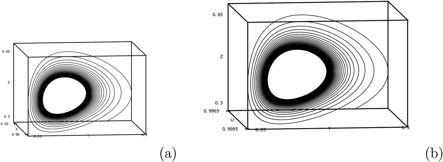
(a) Chaotic solution in
(a) Periodic limit cycle solution in

Time series of the system (2) for

Time series of the system (2) for
These observations indicate that the additional prey could be used as a biological control parameter for controlling chaotic dynamics.
We consider the following data:
In the absence of additional prey

Limit cycle in
However, by providing additional food
The persistence of all four species in the form of chaotic attractors is possible (Figure 7). The system exhibits various dynamical behaviors.

Chaotic solution in
For further increase in

Chaotic solution in
In Figure 9, a bifurcation diagram is plotted with respect to the parameter

Bifurcation diagram of system (2) with respect to parameter
8 Conclusion
A food-web model comprising four species is developed and investigated. The solution is bounded and positively invariant in a closed and bounded domain, reflecting the well-behaved nature of the model. The local stability has been carried out about its various equilibrium points. The survival of all four species is explored, and conditions are established for their persistence. The occurrence of transcritical bifurcation experienced by the system has been discussed analytically. In the context of our study, the occurrence of a transcritical bifurcation may imply that management or conservation efforts need to carefully consider the parameter values to avoid tipping points that lead to undesirable outcomes. For instance, introducing an invasive species or changes in additional food could trigger such shifts, with cascading effects throughout the food web. The numerical simulations reveal rich dynamics in the system, including stable focus, limit cycle, and chaos. Chaos observed in our model involving an additional food underscores the intricate and uncertain dynamics inherent to ecological systems. This chaotic behavior results from intricate, nonlinear interactions among species and can significantly impact ecological aspects such as biodiversity, stability, and managing natural ecosystems. The appropriate additional food may control the chaos in classical Hasting’s model, giving a stable focus where all four species survive.
-
Funding information: The first author would like to thank the Council of Scientific and Industrial Research, New Delhi, Government of India (File No. 09/143(0902)/2017 EMR-I), for financial support to carry out her research work and the Department of Mathematics, Indian Institute of Technology Roorkee (IIT Roorkee), for providing stimulating scientific environment and resources. The work of Anuraj Singh is supported by a Core Research Grant, Science Engineering Research Board, Govt. of India (CRG/2021/006380).
-
Conflict of interest: The authors declare that they have no conflict of interest.
-
Ethical approval: This research did not require ethical approval.
References
[1] Birkhoff, G, & Rota, JC. (1989). Ordinary Differential Equations, New York, NY: John Wiley. Search in Google Scholar
[2] Creel, S., & Christianson, D. (2008). Relationships between direct predation and risk effects. Trends in Ecology & Evolution, 23(4), 194–201. 10.1016/j.tree.2007.12.004Search in Google Scholar PubMed
[3] Debnath, S., Ghosh, U., & Sarkar, S. (2020). Global dynamics of a tritrophic food chain model subject to the Allee effects in the prey population with sexually reproductive generalized-type top predator. Computational and Mathematical Methods, 2(2), e1079. 10.1002/cmm4.1079Search in Google Scholar
[4] Gakkhar, S., & Singh, A. (2012). Control of chaos due to additional predator in the Hastings-Powell food chain model. Journal of Mathematical Analysis and Applications, 385(1), 423–438. 10.1016/j.jmaa.2011.06.047Search in Google Scholar
[5] Ghosh, U., Pal, S., & Banerjee, M. (2021). Memory effect on Bazykin’s prey-predator model: Stability and bifurcation analysis. Chaos, Solitons & Fractals, 143, 110531. 10.1016/j.chaos.2020.110531Search in Google Scholar
[6] Gilpin, M. E. (1979). Spiral chaos in a predator-prey model. The American Naturalist, 113(2), 306–308. 10.1086/283389Search in Google Scholar
[7] Haque, M., & Venturino, E. (2007). An ecoepidemiological model with disease in predator: the ratio-dependent case. Mathematical methods in the Applied Sciences, 30(14), 1791–1809. 10.1002/mma.869Search in Google Scholar
[8] Hastings, A., & Powell, T. (1991). Chaos in a three-species food chain. Ecology, 72(3), 896–903. 10.2307/1940591Search in Google Scholar
[9] Holling, C. S. (1959). The components of predation as revealed by a study of small-mammal predation of the European pine sawfly1. The Canadian Entomologist, 91(5), 293–320. 10.4039/Ent91293-5Search in Google Scholar
[10] Holmes, E. E., Lewis, M. A., Banks, J., & Veit, R. (1994). Partial differential equations in ecology: spatial interactions and population dynamics. Ecology, 75(1), 17–29. 10.2307/1939378Search in Google Scholar
[11] Kot, M. (2001). Elements of Mathematical Ecology. Cambridge: Cambridge University Press. 10.1017/CBO9780511608520Search in Google Scholar
[12] Lotka, A. (1925). Elements of physical biology. Baltimore: Williams and Wilkins. p. 460. Search in Google Scholar
[13] Meng, X., Liu, R., & Zhang, T. (2014). Adaptive dynamics for a non-autonomous Lotka-Volterra model with size-selective disturbance. Nonlinear Analysis: Real World Applications, 16, 202–213. 10.1016/j.nonrwa.2013.09.019Search in Google Scholar
[14] Morozov, A., Petrovskii, S., & Li, B.-L. (2004). Bifurcations and chaos in a predator-prey system with the Allee effect. Proceedings of the Royal Society of London. Series B: Biological Sciences, 271(1546), 1407–1414. 10.1098/rspb.2004.2733Search in Google Scholar PubMed PubMed Central
[15] Murray, J. D. (2001). Mathematical biology II: spatial models and biomedical applications, vol. 3, New York: Springer. Search in Google Scholar
[16] Perc, M., & Szolnoki, A. (2007). Noise-guided evolution within cyclical interactions. New Journal of Physics, 9(8), 267. 10.1088/1367-2630/9/8/267Search in Google Scholar
[17] Perko, L. (1996). Nonlinear systems: Local theory in differential equations and dynamical systems. Newyork: Springer Science and Business Media. pp. 65–178. 10.1007/978-1-4684-0249-0_2Search in Google Scholar
[18] Prasad, B., Banerjee, M., & Srinivasu, P. (2013). Dynamics of additional food provided predator-prey system with mutually interfering predators. Mathematical Biosciences, 246(1), 176–190. 10.1016/j.mbs.2013.08.013Search in Google Scholar PubMed
[19] Sahoo, B., & Poria, S. (2014). The chaos and control of a food chain model supplying additional food to top-predator. Chaos, Solitons & Fractals, 58, 52–64. 10.1016/j.chaos.2013.11.008Search in Google Scholar
[20] Sahoo, B., & Poria, S. (2015). Effects of additional food in a delayed predator-prey model. Mathematical Biosciences, 261, 62–73. 10.1016/j.mbs.2014.12.002Search in Google Scholar PubMed
[21] Samanta, S., Mandal, A. K., Kundu, K., & Chattopadhyay, J. (2014). Control of disease in prey population by supplying alternative food to predator. Journal of Biological Systems, 22(04), 677–690. 10.1142/S0218339014500272Search in Google Scholar
[22] Schaffer, W. M., & Kot, M. (1986). Differential systems in ecology and epidemiology. Chaos, 8, 158–178. 10.1515/9781400858156.158Search in Google Scholar
[23] Singh, A., Tripathi, D., & Kang, Y. (2023). A modified may Holling tanner model: The role of dynamic alternative resources on species’ survival. Journal of Biological Systems, 32, 2450007. 10.1142/S0218339024500074Search in Google Scholar
[24] Tiwari, V., Tripathi, J. P., Jana, D., Tiwari, S. K., & Upadhyay, R. K. (2020). Exploring complex dynamics of spatial predator-prey system: Role of predator interference and additional food. International Journal of Bifurcation and Chaos, 30(7), 2050102. 10.1142/S0218127420501023Search in Google Scholar
[25] Tripathi, D., & Singh, A. (2023). An eco-epidemiological model with predator switching behavior. Computational and Mathematical Biophysics, 11(1), 20230101. 10.1515/cmb-2023-0101Search in Google Scholar
[26] Tripathi, J. P., Abbas, S., & Thakur, M. (2015). Dynamical analysis of a prey-predator model with Beddington-Deangelis type function response incorporating a prey refuge. Nonlinear Dynamics, 80, 177–196. 10.1007/s11071-014-1859-2Search in Google Scholar
[27] Tripathi, J. P., Tripathi, D., Mandal, S., & Shrimali, M. D. (2023). Cannibalistic enemy-pest model: effect of additional food and harvesting. Journal of Mathematical Biology, 87(4), 58. 10.1007/s00285-023-01991-9Search in Google Scholar PubMed
[28] Wang, X., Zanette, L., & Zou, X. (2016). Modelling the fear effect in predator-prey interactions. Journal of Mathematical Biology, 73(5), 1179–1204. 10.1007/s00285-016-0989-1Search in Google Scholar PubMed
[29] Wang, X., & Zhao, M. (2011). Complex dynamics in a ratio-dependent food-chain model with Beddington-Deangelis functional response. Procedia Environmental Sciences, 10, 135–140. 10.1016/j.proenv.2011.09.024Search in Google Scholar
[30] Yin, C., Chen, Y., & Zhong, S.-M. (2014). Fractional-order sliding mode based extremum seeking control of a class of nonlinear systems. Automatica, 50(12), 3173–3181. 10.1016/j.automatica.2014.10.027Search in Google Scholar
[31] Zanette, L. Y., White, A. F., Allen, M. C., & Clinchy, M. (2011). Perceived predation risk reduces the number of offspring songbirds produce per year. Science, 334(6061), 1398–1401. 10.1126/science.1210908Search in Google Scholar PubMed
[32] Zhang, T., & Zang, H. (2014). Delay-induced Turing instability in reaction-diffusion equations. Physical Review E, 90(5), 052908. 10.1103/PhysRevE.90.052908Search in Google Scholar PubMed
© 2023 the author(s), published by De Gruyter
This work is licensed under the Creative Commons Attribution 4.0 International License.
Articles in the same Issue
- Special Issue: Infectious Disease Modeling In the Era of Post COVID-19
- A comprehensive and detailed within-host modeling study involving crucial biomarkers and optimal drug regimen for type I Lepra reaction: A deterministic approach
- Application of dynamic mode decomposition and compatible window-wise dynamic mode decomposition in deciphering COVID-19 dynamics of India
- Role of ecotourism in conserving forest biomass: A mathematical model
- Impact of cross border reverse migration in Delhi–UP region of India during COVID-19 lockdown
- Cost-effective optimal control analysis of a COVID-19 transmission model incorporating community awareness and waning immunity
- Evaluating early pandemic response through length-of-stay analysis of case logs and epidemiological modeling: A case study of Singapore in early 2020
- Special Issue: Application of differential equations to the biological systems
- An eco-epidemiological model with predator switching behavior
- A numerical method for MHD Stokes model with applications in blood flow
- Dynamics of an eco-epidemic model with Allee effect in prey and disease in predator
- Optimal lock-down intensity: A stochastic pandemic control approach of path integral
- Bifurcation analysis of HIV infection model with cell-to-cell transmission and non-cytolytic cure
- Special Issue: Differential Equations and Control Problems - Part I
- Study of nanolayer on red blood cells as drug carrier in an artery with stenosis
- Influence of incubation delays on COVID-19 transmission in diabetic and non-diabetic populations – an endemic prevalence case
- Complex dynamics of a four-species food-web model: An analysis through Beddington-DeAngelis functional response in the presence of additional food
- A study of qualitative correlations between crucial bio-markers and the optimal drug regimen of Type I lepra reaction: A deterministic approach
- Regular Articles
- Stochastic optimal and time-optimal control studies for additional food provided prey–predator systems involving Holling type III functional response
- Stability analysis of an SIR model with alert class modified saturated incidence rate and Holling functional type-II treatment
- An SEIR model with modified saturated incidence rate and Holling type II treatment function
- Dynamic analysis of delayed vaccination process along with impact of retrial queues
- A mathematical model to study the spread of COVID-19 and its control in India
- Within-host models of dengue virus transmission with immune response
- A mathematical analysis of the impact of maternally derived immunity and double-dose vaccination on the spread and control of measles
- Influence of distinct social contexts of long-term care facilities on the dynamics of spread of COVID-19 under predefine epidemiological scenarios