A study of qualitative correlations between crucial bio-markers and the optimal drug regimen of Type I lepra reaction: A deterministic approach
-
Dinesh Nayak


Abstract
Mycobacterium leprae is a bacterium that causes the disease leprosy (Hansen’s disease), which is a neglected tropical disease. More than 2,00,000 cases are being reported per year worldwide. This disease leads to a chronic stage known as lepra reaction that majorly causes nerve damage of the peripheral nervous system leading to loss of organs. The early detection of this lepra reaction through the level of bio-markers can prevent this reaction occurring and the further disabilities. Motivated by this, we frame a mathematical model considering the pathogenesis of leprosy and the chemical pathways involved in lepra reactions. The model incorporates the dynamics of the susceptible Schwann cells, infected Schwann cells, and the bacterial load and the concentration levels of the bio-markers
1 Introduction
Leprosy, the oldest disease known to human civilization, is one of the highly neglected tropical diseases caused by a slow-growing bacterium called Mycobacterium leprae (M. leprae). Mainly, this bacterium causes damage to the Schwann cells and hence the skin; thereby, the peripheral nervous system of host body gets impacted. It also has bad impact on eyes and mucosa of the upper respiratory tract. The report of World Health Organization (WHO) states that about 120 countries are still reporting new cases of leprosy which accounts to more than 2,00,000 per year [39]. In the year 2021, India alone spotted about 75,395 new cases [38]. Leprosy disease can lead to a chronic phase of lepra reaction that causes permanent disabilities and loss of organs. Early detection of the disease by observing the key changes in the bio-marker level will play a vital role to prevent the losses.
The chemical and metabolic properties of the cytosol environment of host cell that gets altered in the presence of the M. leprae were first explained by Rudolf Virchow (1821–1902) in the late nineteenth century [37]. Furthermore, different clinical studies explained about the pathway of cytokine responses based upon which there are mainly two types of lepra reactions. The Type-1 lepra reactions are associated with cellular immune response, whereas Type 2 reactions are associated with humoral immune response [3,24]. Both these pathways involve the crucial bio-markers/cytokines such as
There are quite a number of biochemical studies that deal with the pathogenesis of lepra reaction [29] and some on growth of the bacteria and chemical consequences [30]. On the mathematical modeling front, it can be seen that modeling of leprosy began in the 1970s with simple compartmental models, such as the susceptible-infectious-recovered framework [18]. Later, various complex models were framed to evaluate the effectiveness of long-term control and elimination strategies, such as mass drug administration, contact tracing, and vaccination [19]. The very first stochastic leprosy model to investigate uncertainties in leprosy epidemiology was developed in 1999 [27]. This modeling framework is known as simulation model for leprosy transmission and control (SIMLEP) model. This SIMLEP model was further developed to include the disease dynamics in households and heterogeneity in susceptibility, and a new individual-based model stochastic individual-based model on control of leprosy was proposed [10].
In addition to these individual-based models, a mathematical simulation model was studied with a delay time taken into account during the development of the disease [15]. Furthermore, some population studies that combine a simple leprosy model with a tuberculosis model for exploring the contribution of the immunity acquired from tuberculosis to the disappearance of leprosy in Western Europe can be found in [23]. The work [4] deals with a comprehensive review of population models in leprosy. The mathematical models developed for Leprosy are also used for understanding the 65 cancer immunosurveillance and T cell energy [34].
From the literature, we see that limited studies explore the cellular dynamics of leprosy. The very first within-host model for leprosy predicts the actual role of M. leprae bacteria for the infection on human Schwann cells and dissemination of the disease leprosy [12]. The work [13] formulates a three-compartment within-host leprosy model and studies the effects of the density-dependent parameter on M. leprae. The work [14] deals with a four-compartment within-host leprosy model and concludes that the process of demyelination, nerve regeneration, and infection of the healthy Schwann cells are the three most crucial factors in the pathogenesis of leprosy. The authors in previous work [28] presented a comprehensive and detailed within-host modeling study involving crucial biomarkers and optimal drug regimen for Type I lepra reaction. These models help researchers better understand the nuances of leprosy epidemiology and its implications for control and treatment strategies.
To our knowledge, there is no work performed yet dealing with the dynamics of the bio-markers involved in lepra reactions. Also, there seems to be neither any clinical work that clearly deals with the dynamics of bio-markers during lepra reactions. Hence, it is extremely important to study the dynamics at the bio-markers levels and their correlation with the multidrug therapy (MDT) drugs that can help the clinicians for control of occurrence of lepra reactions.
Motivated by these observations in this work, we propose to study the dynamics of the bio-markers through chemical reactions. In the next section, we discuss and detail the proposed mathematical model. We use the drugs in MDT as control variables. We frame an optimal control problem along with a cost function
2 Mathematical model formulation
Based on the clinical literature, we consider a model that consists of susceptible Schwann cells
Similar formulations are used for studying the concentration levels of IL-12, IL-15, and IL-17 compartments by equations (7)–(9), respectively.
2.1 Description of the control variables dealing with the MDT drugs
WHO guidelines 2018 recommends an MDT for leprosy that consist of three drugs rifampin, dapsone, and clofazimine [25,36]. The impact of each of these drugs and their mathematical articulation as control variables is as follows:
Rifampin (
Dapsone (
Clofazimine (
We next propose the mathematical model dealing with the mechanism of drug action on each compartment of susceptible cells, infected cells, and bacterial load along with concentration level of the cytokines.
| Symbols | Biological meaning |
|---|---|
|
|
Susceptible Schwann cells |
|
|
Infected Schwann cells |
|
|
Bacterial load |
|
|
Concentration of IFN-
|
|
|
Concentration of TNF-
|
|
|
Concentration of IL-12 |
|
|
Concentration of IL-15 |
|
|
Concentration of IL-17 |
|
|
Natural birth rate of the susceptible cells |
|
|
Rate at which Schwann cells are infected |
|
|
Death rate of the susceptible cells due to cytokines |
|
|
Natural death rate of Schwann cells and infected Schwann cells |
|
|
Death rate of infected Schwann cells due to cytokines |
|
|
Burst rate of infected Schwann cells realising the bacteria |
|
|
Rates at which M. leprae is removed by cytokines |
|
|
Natural death rate of M. leprae |
|
|
Production rate of IFN-
|
|
|
Inhibition of IFN-
|
|
|
Inhibition of IFN-
|
|
|
Inhibition of IFN-
|
|
|
Inhibition of IFN-
|
|
|
Decay rate of IFN-
|
|
|
Production rate of TNF-
|
|
|
Decay rate of TNF-
|
|
|
Production rate of
|
|
|
Inhibition
|
|
|
Decay rate of
|
|
|
Production rate of
|
|
|
Decay rate of
|
|
|
Production rate of
|
|
|
Decay rate of
|
|
|
Production rate of
|
|
|
Decay rate of
|
|
|
Quantity of
|
|
|
Quantity of
|
|
|
Quantity of
|
|
|
Quantity of
|
|
|
Quantity of
|
|
|
Quantity of
|
Now, mathematically, we define the set of all control variables as follows:
where
Since the drugs in MDT can lead to some hazards, we consider a cost functional that minimizes the drug concentrations along with the infected cell count and the bacterial load.
Based on this, we define the following cost functional:
where the integrand of the cost functional
which denotes the running cost and is commonly known as Lagrangian of the optimal control problem.
Now, the admissible set of solution of the aforementioned optimal control problems (1)–(10) is given by:
where
We next validate the model using 2D heat plots with control variables as zero.
3 Model validation through 2D heat plots
We validate the above-framed model based on the clinical characteristics of leprosy. From the clinical studies, it can be seen that the doubling rate the bacteria (M. leprae) is approximately 14 days [20]. We use this clinical characteristic to validate our model.
To generate these heat plots, we use two pairs of parameters and their range of variation. We consider the pairs of parameters
Values of the parameters complied from clinical literature
| Symbols | Values | Units |
|---|---|---|
|
|
0.0220 [17] |
|
|
|
3.4400 [16] |
|
|
|
0.1795 [30] |
|
|
|
0.0018 [30] |
|
|
|
0.2681 [30] |
|
|
|
0.0630 [20] |
|
|
|
0.0003 [12] |
|
|
|
0.5700 [1] |
|
|
|
0.0003 [31] |
|
|
|
0.005540* |
|
|
|
0.009030* |
|
|
|
0.006250* |
|
|
|
0.004990* |
|
|
|
2.1600 [31] |
|
|
|
0.0040 [31] |
|
|
|
1.1120 [31] |
|
|
|
0.0440 [21] |
|
|
|
0.001460* |
|
|
|
16.000 [21] |
|
|
|
0.0110 [21] |
|
|
|
1.8800 [31] |
|
|
|
0.0250 [34] |
|
|
|
2.1600 [34] |
|
|
|
0.0290 [34] |
|
|
|
2.3400 [34] |
|
|
|
0.1000 [35] | Relative concentration |
|
|
0.1400 [6] | Relative concentration |
|
|
0.1500 [35] | Relative concentration |
|
|
1.1100 [6] | Relative concentration |
|
|
0.2000 [6] | Relative concentration |
|
|
0.3170 [6] | Relative concentration |
The (*) marked values of the parameters are assumed.
In Figure 1(a), the value of

Heat plots: (a) taking
4 Existence of an optimal solution
In this section, we establish the existence of solution for the optimal control Problems (1)–(10) using the existence Theorem 2.2 of [5].
Theorem 1
There exists an 8-tuple of optimal controls (
corresponding to the control Systems (1)–(10), where
Proof
We consider
is a continuous function of
Now, we intend to show that
F1: Here, each of the
F2: We consider
Thus,
Here,
Similarly, for
Now, for
Hence,
But to satisfy this hypothesis for remaining
Similarly, taking
Hence, we are done in satisfying the hypothesis F2.
F3: Since
Now, we have to show that the running cost function
satisfies conditions (
Here,
C1: We see that
C2:
C3: Consider
C4: Since
C5: Using the similar type of argument, we can easily show that for each fixed
Hence, we have shown that the optimal control problem satisfies all the hypothesis of Theorem 2.2 of [5]. Therefore, there exists a 8-tuple of optimal controls
5 Numerical studies for the optimal control problem
5.1 Theory
Here, we discuss the technique to evaluate the aforementioned optimal control problem. To evaluate the optimal control variables and the optimal state variables, we use the forward backward sweep method [26] and the Pontryagin maximum principle [22].
The Hamiltonian of the control Systems (1)–(10) is given by:
where
Now, using the Pontryagin maximum principle with
Clearly, (13) will be equivalent to the control Systems (1)–(10) and system of ordinary differential equations for co-state variables should satisfy the following:
and the transversality condition
Now, to obtain the optimal value of the controls, we use the Newton’s gradient method for optimal control problem [9]. In the following, we discuss briefly on the go about of this method dealing with the iterative update of the control inputs for either minimizing or maximizing the objective function.
This process typically involves the following steps:
Calculate the gradient of the objective function with respect to the control inputs
Update the control inputs by moving in a direction that reduces the objective function value. This is performed through the line search optimization technique in this work. The equation is given in (17).
Solve the state equations for the new control inputs to obtain the corresponding state trajectories. We solved these equations using the Runge-Kutta fourth-order method.
Evaluate the objective function for the updated control inputs and state trajectories.
Check for convergence by comparing the change in the objective function value with a predefined tolerance. If the change is small, the optimization is considered complete.
As mentioned earlier for our case, we use the following recursive formula for updating the control in each step of numerical simulation, i.e.,
where
Now, to execute the aforementioned idea, we have to calculate the gradient for each control, i.e.,
5.2 Numerical simulations
In this section, we perform the numerical simulations to study the correlation of cytokine levels in Type 1 lepra reaction and the drugs involved in MDT in a qualitative manner.
The values of the parameters used are collected from various clinical articles and appropriate references are cited in Table 1. For some of the parameters such as
We then divide these rate percentages by 100 to obtain the values of these parameters. Some of the cases we have taken average of the result yield from different medium such as
For these simulations, we consider the time duration of 100 days, i.e., (
First, we have solved the system numerically without any drug intervention. All the numerical calculations were made in MATLAB, and we used the fourth-order Runge-Kutta method to solve the system of ODEs and to find the value of the
Furthermore, to simulate the system with controls, we use the forward-backward sweep method starting with the initial value of the controls as zero and estimate the state variables forward in time. Since the transversality conditions have the value of adjoint vector at end time
Using the value of state variables and adjoint vector, we calculate the control variables at each time instance that get updated in each iteration. The strategy to update controls is followed by implementing the Newton’s gradient method as expressed in equation (17). We continue this till the convergence criterion is met as in [9].
The weights
Hazard ratio of the drugs
| Drugs | Hazard ratio | Source |
|---|---|---|
| Rifampin | 0.26 | [2] |
| Dapsone | 0.99 | [8] |
| Clofazimine | 1.85 | [8] |
We now numerically simulate the
5.3 Findings
In each of the figures discussed in this section, the first three frames (1–3) depict the dynamics of the respective compartments in Models (1)–(9) with individual drug administration, a combination of administration of two drugs, and all the three drugs in MDT administration, respectively, as control variables/interventions. The further frames in the following are the magnified versions of either Frame-1 and Frame-2 or Frame-1, Frame-2 and Frame-3 and are depicted for better clarity purpose to the reader.
Figure 2 depicts the dynamics of the susceptible cells
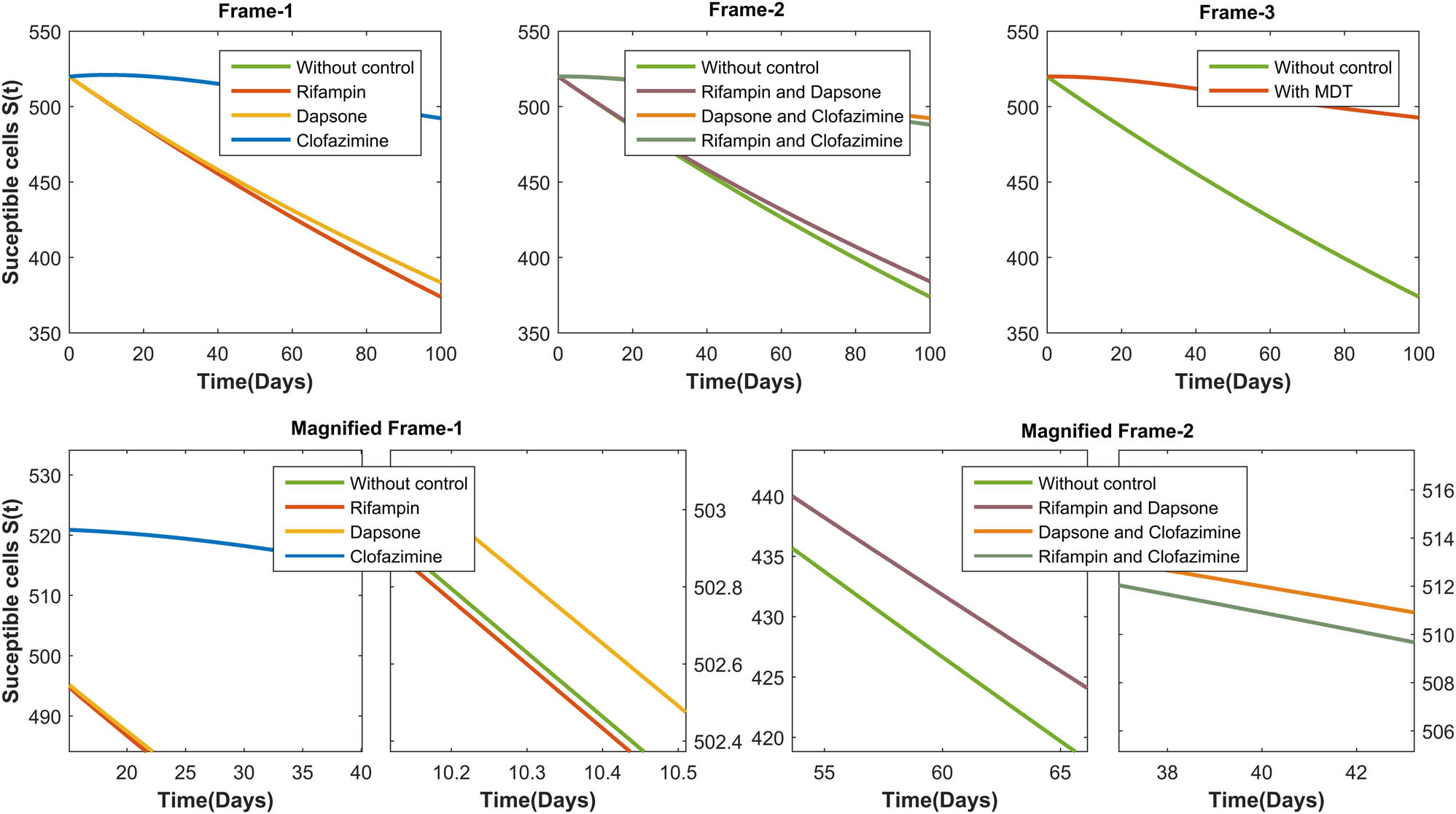
Plot depicting the dynamics of the susceptible cells
Figure 3 depicts the dynamics of the infected cells
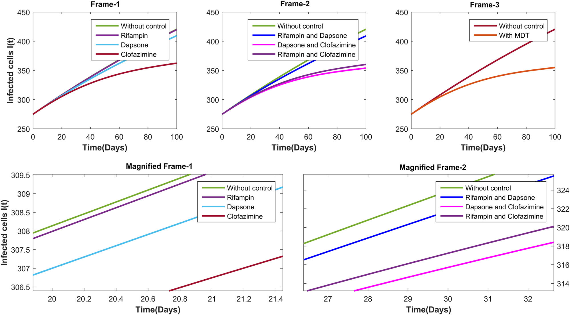
Plot depicting the dynamics of the infected cells
From the magnifications in Figure 4, we see that clofazimine is the most effective and rifampin is the least effective drug in reducing the bacterial load when drugs are administered individually. In case administration of combination of two drugs, dapsone and clofazimine combination, has the most impact and rifampin and dapsone has the least impact, all the three drugs of MDT when administered in combination reduce the bacterial load the best.
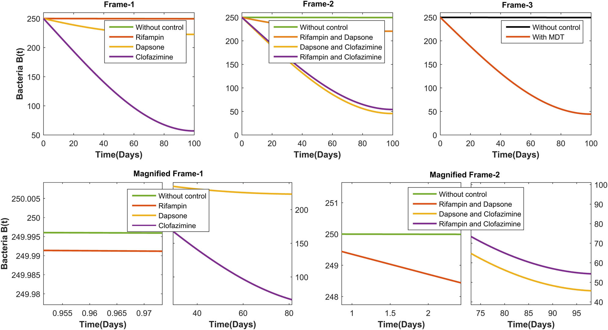
Plot depicting the dynamics of the bacterial load
Figure 5 provides us the most important information that without any intervention of drugs, the level of

Plot depicting the dynamics of the
Figure 6 clearly depicts that the level of TNF-
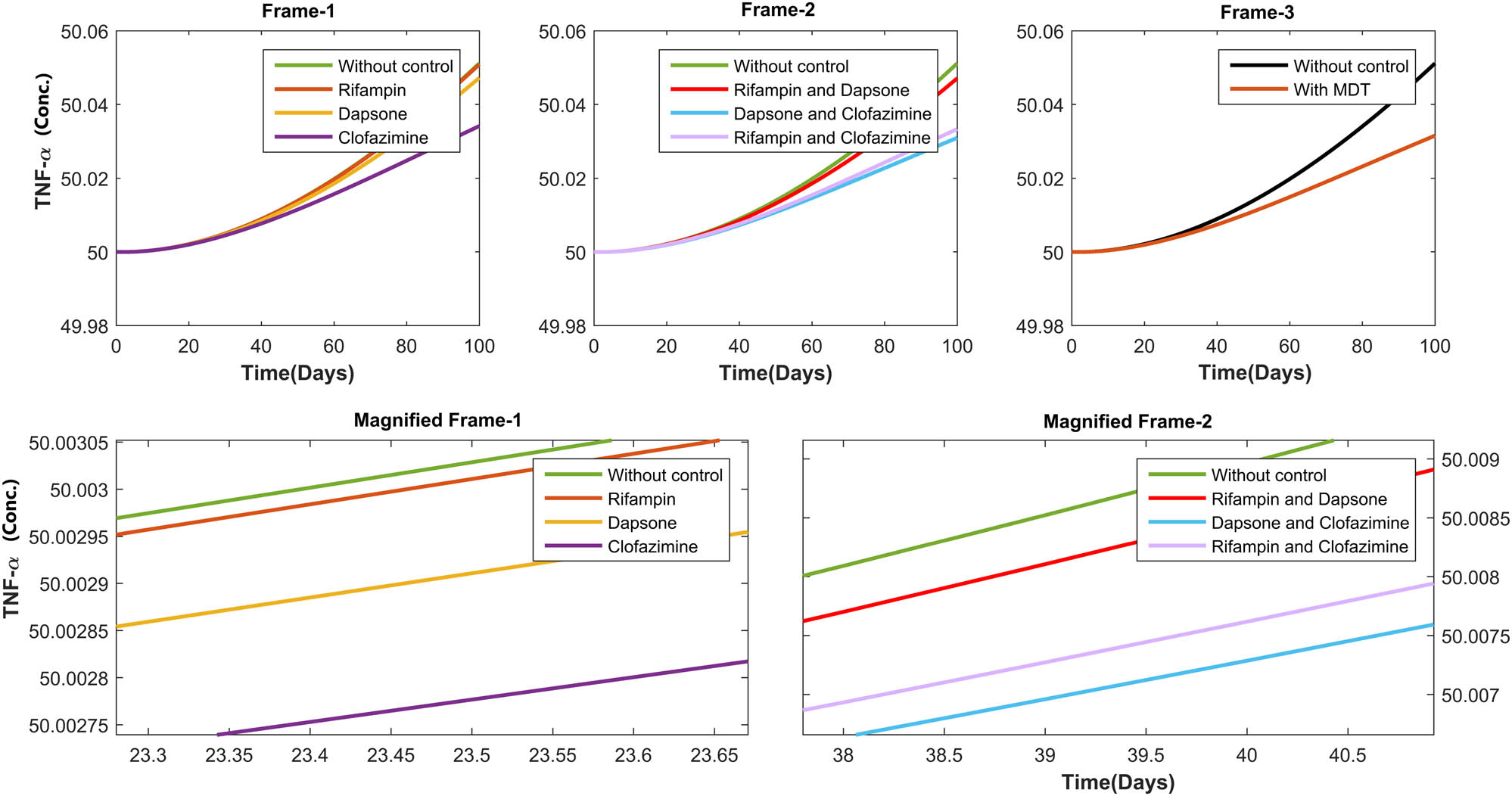
Plot depicting the dynamics of the TNF-

Plot depicting the dynamics of the
Plot depicting the dynamics of the
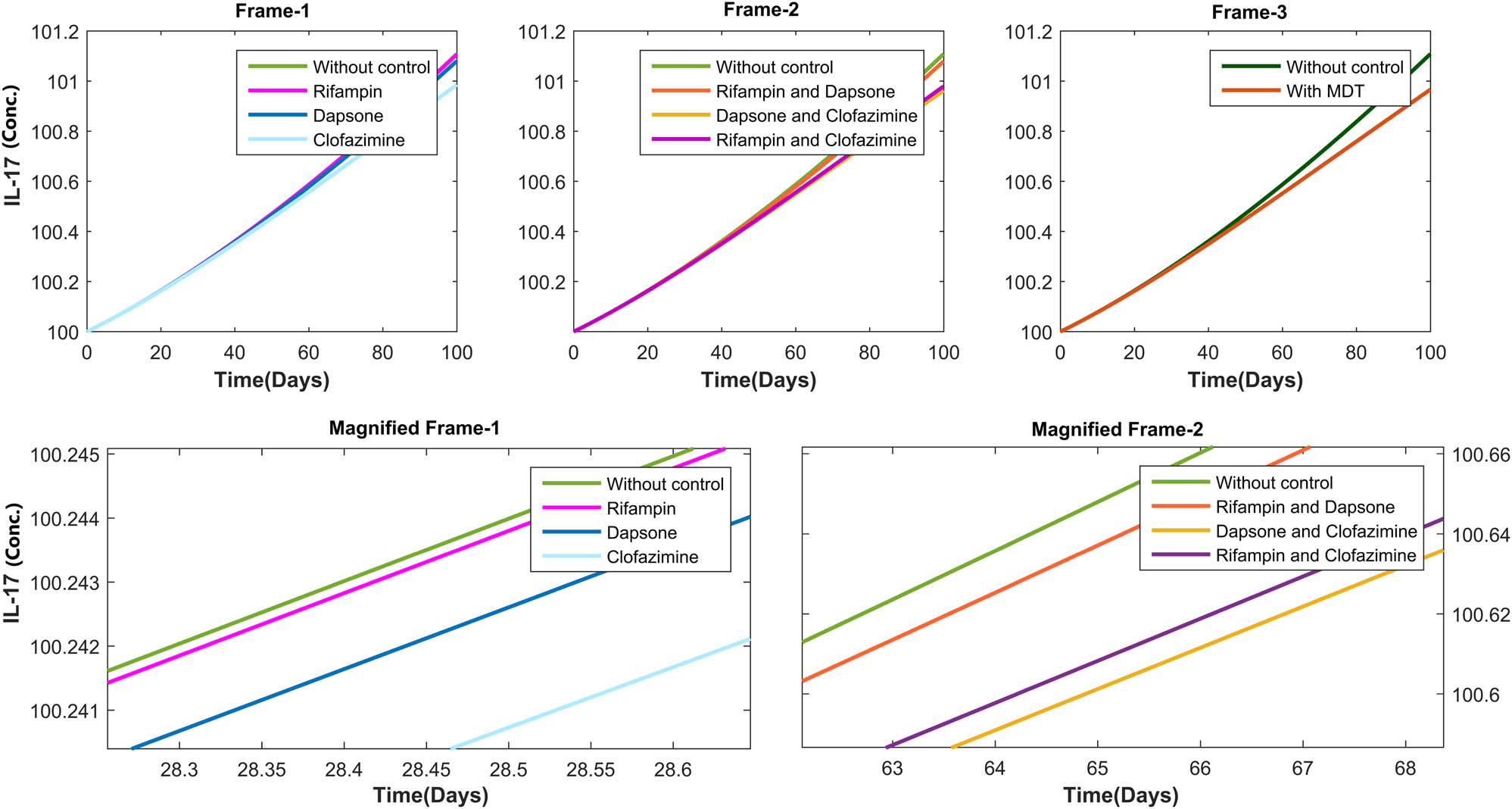
From Figures 9 and 10, it can be seen that during lepra reaction, the levels of both

Plot depicting the dynamics of the

Plot depicting the dynamics of the
6 Discussion and conclusions
The novel thing about this article is that it deals with a model that includes the dynamics of the levels of crucial cytokines that are involved in Type 1 lepra reaction, and also, this work studies the impact of different drugs in MDT on the levels of these cytokines. The findings of the studies includes the following:
Among the drugs used in MDT for treating leprosy, clofazimine and dapsone increase the susceptible cell count, whereas rifampin has a negative impact on it.
The two drug combination of rifampin and dapsone has the negative impact on susceptible cell count.
The MDT drug combinations decrease both the infected cell count and the bacterial load. Clofazimine works the best in reduction when each of the drugs is administered individually, and in combination of two drug administration, a combination of clofazimine and dapsone reduces the best.
During the Type I lepra reaction, the levels of
Each of the drugs used in MDT enhances the
The levels of both the cytokines
In the case of TFN-
In summary, this is a novel and first of its kind work wherein we have discussed the natural history and dynamics of crucial bio-markers in a Type I lepra reaction and also studied in detail the influence of different combinations of drugs in MDT used for treating leprosy on the levels of these bio-makers. This study can be of important help to the clinician in early detection of the leprosy and avoid and control the disease from going to lepra reactions and help in averting major damages.
Acknowledgements
The authors dedicate this article to the Founder Chancellor of SSSIHL, Bhagawan Sri Sathya Sai Baba. The corresponding author also dedicates this article to his loving elder brother D.A.C. Prakash who still lives in his heart.
-
Funding information: This research was supported by Council of Scientific and Industrial Research (CSIR) under project grant – Role and Interactions of Biological Markers in Causation of Type1/Type 2 Lepra Reactions: A In Vivo Mathematical Modelling with Clinical Validation (Sanction Letter No. 25(0317)/20/EMR-II).
-
Conflict of interest: The authors declare no conflict of interest for this research work.
-
Ethical approval: This research did not require any ethical approval.
-
Data availability statement: We do not analyze or generate any datasets, because our work proceeds within a theoretical and mathematical approach.
References
[1] Almeida, J.G. (1992). A quantitative basis for sustainable anti-Mycobacterium leprae chemotherapy in leprosy control programs. International Journal of Leprosy and Other Mycobacterial Diseases: Official Organ of the International Leprosy Association, 60(2), 255–268. Search in Google Scholar
[2] Bakker, M. I., Hatta, M., Kwenang, A., Van Benthem, B. H., Van Beers, S. M., …, Oskam, L. (2005). Prevention of leprosy using rifampicin as chemoprophylaxis. The American Journal of Tropical Medicine and Hygiene, 72(4), 443–448. 10.4269/ajtmh.2005.72.443Search in Google Scholar
[3] Bilik, L., Demir, B., & Cicek, D. (2019). Leprosy reactions. Hansen’s Disease-The Forgotten and Neglected Disease. London: IntechOpen.10.5772/intechopen.72481Search in Google Scholar
[4] Blok, D. J., de Vlas, S. J., Fischer, E. A., & Richardus, J. H. (2015). Mathematical modeling of leprosy and its control. Advances in Parasitology, 87, 33–51. 10.1016/bs.apar.2014.12.002Search in Google Scholar PubMed
[5] Boyarsky, A. (1976). On the existence of optimal controls for nonlinear systems. Journal of Optimization Theory and Applications, 20(2), 205–213. 10.1007/BF01767452Search in Google Scholar
[6] Brady, R., Frank-Ito, D. O., Tran, H. T., Janum, S., Moooller, K., Brix, S., …, Olufsen, M. S. (2016). Personalized mathematical model predicting endotoxin-induced inflammatory responses in young men. http://arXiv.org/abs/arXiv:1609.01570. Search in Google Scholar
[7] Bullock, W. E. (1983). Rifampin in the treatment of leprosy. Reviews of Infectious Diseases, 5(Supplement_3), S606–S613. 10.1093/clinids/5.Supplement_3.S606Search in Google Scholar PubMed
[8] Cerqueira, S. R. P. S., Deps, P. D., Cunha, D. V., Bezerra, N. V. F., Barroso, D. H., Pinheiro, A. B. S., …, Gomes, C. M. (2021). The influence of leprosy-related clinical and epidemiological variables in the occurrence and severity of covid-19: A prospective real-world cohort study. PLoS Neglected Tropical Diseases, 15(7), e0009635. 10.1371/journal.pntd.0009635Search in Google Scholar PubMed PubMed Central
[9] Edge, E. R., & Powers, W. F. (1976). Function-space quasi-newton algorithms for optimal control problems with bounded controls and singular arcs. Journal of Optimization Theory and Applications, 20(4), 455–479. 10.1007/BF00933131Search in Google Scholar
[10] Fischer, E. A., de Vlas, S. J., Habbema, J. D. F., & Richardus, J. H. (2011). The long term effect of current and new interventions on the new case detection of leprosy: A modeling study. PLoS Neglected Tropical Diseases, 5(9), e1330. 10.1371/journal.pntd.0001330Search in Google Scholar PubMed PubMed Central
[11] Garrelts, J. C. (1991). Clofazimine: A review of its use in leprosy and Mycobacterium avium complex infection. Dicp, 25(5), 525–531. 10.1177/106002809102500513Search in Google Scholar PubMed
[12] Ghosh, S., Chatterjee, A., Roy, P., Grigorenko, N., Khailov, E., and Grigorieva, E. (2021). Mathematical modeling and control of the cell dynamics in leprosy. Computational Mathematics and Modeling, 32, 1–23. 10.1007/s10598-021-09516-zSearch in Google Scholar
[13] Ghosh, S., Rana, S., & Roy, P. K. (2022). Leprosy: Considering the effects on density-dependent growth of Mycobacterium leprae. Differential Equations and Dynamical Systems (pp. 1–15). Switzerland: Springer. 10.1007/s12591-022-00608-9Search in Google Scholar
[14] Ghosh, S., Saha, S., & Roy, P. K. (2023). Critical observation of who recommended multidrug therapy on the disease leprosy through mathematical study. Journal of Theoretical Biology, 567, 111496. 10.1016/j.jtbi.2023.111496Search in Google Scholar PubMed
[15] Giraldo, L., Garcia, U., Raigosa, O., Munoz, L., Dalia, M. M. P., & Jamboos, T. (2018). Multibacillary and paucibacillary leprosy dynamics: A simulation model including a delay. Applied Mathematical Science, 12(32), 1677–1685. 10.12988/ams.2018.88121Search in Google Scholar
[16] Jin, S.-H., An, S.-K., & Lee, S.-B. (2017). The formation of lipid droplets favors intracellular Mycobacterium leprae survival in sw-10, non-myelinating Schwann cells. PLoS Neglected Tropical Diseases, 11(6), e0005687. 10.1371/journal.pntd.0005687Search in Google Scholar PubMed PubMed Central
[17] Kim, H.-S., Lee, J., Lee, D. Y., Kim, Y.-D., Kim, J. Y., Lim, H. J., …, Cho, Y. S. (2017). Schwann cell precursors from human pluripotent stem cells as a potential therapeutic target for myelin repair. Stem Cell Reports, 8(6), 1714–1726. 10.1016/j.stemcr.2017.04.011Search in Google Scholar PubMed PubMed Central
[18] Lechat, M., Misson, J., Vellut, C., Misson, C., & Bouckaert, A. (1974). An epidemetric model of leprosy. Bulletin of the World Health Organization, 51(4), 361–373. Search in Google Scholar
[19] Lechat, M. F., Misson, C. B., Lambert, A., Bouckaert, A., Vanderveken, M., & Vellut, C. (1985). Simulation of vaccination and resistance in leprosy using an epidemiometric model. International Journal of Leprosy, 53, 461–467. Search in Google Scholar
[20] Levy, L., & Baohong, J. (2006). The mouse foot-pad technique for cultivation of Mycobacterium leprae. Leprosy Review, 77(1), 5–24. 10.47276/lr.77.1.5Search in Google Scholar
[21] Liao, K.-L., Bai, X.-F., & Friedman, A. (2013). The role of cd200-cd200r in tumor immune evasion. Journal of theoretical biology, 328, 65–76. 10.1016/j.jtbi.2013.03.017Search in Google Scholar PubMed
[22] Liberzon, D. (2011). Calculus of variations and optimal control theory: A concise introduction. New Jersey: Princeton University Press. 10.2307/j.ctvcm4g0sSearch in Google Scholar
[23] Lietman, T., Porco, T., & Blower, S. (1997). Leprosy and tuberculosis: The epidemiological consequences of cross-immunity. American Journal of Public Health, 87(12), 1923–1927. 10.2105/AJPH.87.12.1923Search in Google Scholar PubMed PubMed Central
[24] Luo, Y., Kiriya, M., Tanigawa, K., Kawashima, A., Nakamura, Y., Ishii, N., & Suzuki, K. (2021). Host-related laboratory parameters for leprosy reactions. Frontiers in Medicine, 8, 694376. 10.3389/fmed.2021.694376Search in Google Scholar PubMed PubMed Central
[25] Maymone, M. B., Venkatesh, S., Laughter, M., Abdat, R., Hugh, J., Dacso, M. M., …, Dellavalle, R. P. (2020). Leprosy: Treatment and management of complications. Journal of the American Academy of Dermatology, 83(1), 17–30. 10.1016/j.jaad.2019.10.138Search in Google Scholar PubMed
[26] McAsey, M., Mou, L., & Han, W. (2012). Convergence of the forward-backward sweep method in optimal control. Computational Optimization and Applications, 53, 207–226. 10.1007/s10589-011-9454-7Search in Google Scholar
[27] Meima, A., Gupte, M. D., Van Oortmarssen, G. J., & Habbema, J. D. F. (1999). Simlep: A simulation model for leprosy transmission and control. International Journal of Leprosy and Other Mycobacterial Diseases, 67, 215–236. Search in Google Scholar
[28] Nayak, D., Chhetri, B., Vamsi Dasu, K. K., Muthusamy, S., & Bhagat, V. M. (2023). A comprehensive and detailed within-host modeling study involving crucial biomarkers and optimal drug regimen for type i lepra reaction: A deterministic approach. Computational and Mathematical Biophysics, 11(1), 20220148. 10.1515/cmb-2022-0148Search in Google Scholar
[29] Ojo, O., Williams, D. L., Adams, L. B., & Lahiri, R. (2022). Mycobacterium leprae transcriptome during in vivo growth and ex vivo stationary phases. Frontiers in Cellular and Infection Microbiology, 11, 1410. 10.3389/fcimb.2021.817221Search in Google Scholar PubMed PubMed Central
[30] Oliveira, R. B., Sampaio, E. P., Aarestrup, F., Teles, R. M., Silva, T. P., Oliveira, A. L., …, Sarno, E. N. (2005). Cytokines and Mycobacterium leprae induce apoptosis in human Schwann cells. Journal of Neuropathology & Experimental Neurology, 64(10), 882–890. 10.1097/01.jnen.0000182982.09978.66Search in Google Scholar PubMed
[31] Pagalay, U. (2014). A mathematical model for interaction macrophages, t lymphocytes and cytokines at infection of mycobacterium tuberculosis with age influence. International Journal of Science and Technology, 3(3), 5–14. Search in Google Scholar
[32] Paniker, U., & Levine, N. (2001). Dapsone and sulfapyridine. Dermatologic Clinics, 19(1), 79–86. 10.1016/S0733-8635(05)70231-XSearch in Google Scholar PubMed
[33] Parida, S. K., & Grau, G. E. (1993). Role of TNF in immunopathology of leprosy. Research in Immunology, 144, 376–387. 10.1016/S0923-2494(93)80083-BSearch in Google Scholar
[34] Su, B., Zhou, W., Dorman, K., & Jones, D. (2009). Mathematical modeling of immune response in tissues. Computational and Mathematical Methods in Medicine, 10(1), 9–38. 10.1080/17486700801982713Search in Google Scholar
[35] Talaei, K., Garan, S. A., Quintela, B. d. M., Olufsen, M. S., Cho, J., Jahansooz, J. R., …, Lobosco, M. (2021). A mathematical model of the dynamics of cytokine expression and human immune cell activation in response to the pathogen Staphylococcus aureus. Frontiers in Cellular and Infection Microbiology, 11, 1079. 10.3389/fcimb.2021.711153Search in Google Scholar PubMed PubMed Central
[36] Tripathi, K. (2013). Essentials of medical pharmacology. New Delhi: JP Medical Ltd. 10.5005/jp/books/12256Search in Google Scholar
[37] Virchow, R. (1865). Die krankhaften Geschwülste: 30 Vorlesungen, geh. während d. Wintersemesters 1862–1863 an d. Univ. zu Berlin (Vol. 2). Berlin: Hirschwald. Search in Google Scholar
[38] WHO. (2022). Number of new leprosy cases in 2021. Search in Google Scholar
[39] WHO. (2023). Leprosy. Search in Google Scholar
© 2023 the author(s), published by De Gruyter
This work is licensed under the Creative Commons Attribution 4.0 International License.
Articles in the same Issue
- Special Issue: Infectious Disease Modeling In the Era of Post COVID-19
- A comprehensive and detailed within-host modeling study involving crucial biomarkers and optimal drug regimen for type I Lepra reaction: A deterministic approach
- Application of dynamic mode decomposition and compatible window-wise dynamic mode decomposition in deciphering COVID-19 dynamics of India
- Role of ecotourism in conserving forest biomass: A mathematical model
- Impact of cross border reverse migration in Delhi–UP region of India during COVID-19 lockdown
- Cost-effective optimal control analysis of a COVID-19 transmission model incorporating community awareness and waning immunity
- Evaluating early pandemic response through length-of-stay analysis of case logs and epidemiological modeling: A case study of Singapore in early 2020
- Special Issue: Application of differential equations to the biological systems
- An eco-epidemiological model with predator switching behavior
- A numerical method for MHD Stokes model with applications in blood flow
- Dynamics of an eco-epidemic model with Allee effect in prey and disease in predator
- Optimal lock-down intensity: A stochastic pandemic control approach of path integral
- Bifurcation analysis of HIV infection model with cell-to-cell transmission and non-cytolytic cure
- Special Issue: Differential Equations and Control Problems - Part I
- Study of nanolayer on red blood cells as drug carrier in an artery with stenosis
- Influence of incubation delays on COVID-19 transmission in diabetic and non-diabetic populations – an endemic prevalence case
- Complex dynamics of a four-species food-web model: An analysis through Beddington-DeAngelis functional response in the presence of additional food
- A study of qualitative correlations between crucial bio-markers and the optimal drug regimen of Type I lepra reaction: A deterministic approach
- Regular Articles
- Stochastic optimal and time-optimal control studies for additional food provided prey–predator systems involving Holling type III functional response
- Stability analysis of an SIR model with alert class modified saturated incidence rate and Holling functional type-II treatment
- An SEIR model with modified saturated incidence rate and Holling type II treatment function
- Dynamic analysis of delayed vaccination process along with impact of retrial queues
- A mathematical model to study the spread of COVID-19 and its control in India
- Within-host models of dengue virus transmission with immune response
- A mathematical analysis of the impact of maternally derived immunity and double-dose vaccination on the spread and control of measles
- Influence of distinct social contexts of long-term care facilities on the dynamics of spread of COVID-19 under predefine epidemiological scenarios