Application of dynamic mode decomposition and compatible window-wise dynamic mode decomposition in deciphering COVID-19 dynamics of India

2.1 Data

The dataset, which is used for the analysis of the novel COVID-19 virus, has been retrieved from https://data.covid19india.org/ [2]. This dataset consists of confirmed cases of 640 Indian districts from April 26, 2020, to October 31, 2021. The columns of this data matrix comprise dates (in increasing order) and the rows comprise the districts, i.e., the rows represent spatial locations and the columns represent temporal locations. Mathematically, the matrix is given by: X = x 0 x 1 x 2 ⋯ x m − 1 x m , where x k ∈ R n for all k ∈ [ 0 , m ] . X can be rewritten as two data matrices as follows:

In this study, we used two datasets, one of which comprise Indian district’s datewise cumulative data (Dataset A), and the other dataset (which is converted from previous dataset), contains state’s weekwise cumulative data (Dataset B). Both the datasets have been arranged as shown in Figure 2.

Figure 2

Dataset A represents districts vs dates matrix of order 640 × 554 , which is converted to Dataset B, which represents states vs weeks matrix of order 36 × 79 .

2.2 DMD

DMD is a spatial dimensionality reduction algorithm that analyzes the relationship between the future data measurement x k + 1 and the previous data measurement x k . We find a linear operator A ∈ R n × n that satisfies the following relation:

for all pairs of data. Depending on the data, it can already be assumed that operator A might not be exact and hence, the relation in equation (1) can generally be described in matrix form.

where † represents the pseudoinverse of the matrix and ‖ . ‖ F is the Frobenius norm. The pseudoinverse is computed using the singular value decomposition (SVD) with rank r truncation:

where U r ∈ R n × r , Σ r ∈ R r × r , V r ∈ R r × m , and ∗ denotes the Hermitian transpose of a matrix. Thus, the matrix A may be solved as follows:

An approximation of the operator A can be found using equations (3) and (4) and choosing a truncation value r as follows:

where A ˜ is the reduced matrix formed by reducing dimension of operator A . It becomes computationally efficient to compute the eigendecomposition of the reduced operator A ˜ , given by: A ˜ W = W Λ , where W are the reduced eigenvectors and Λ are the eigenvalues. The eigenvectors of the full matrix A can thus be computed and is given by:

Φ is known as the DMD mode [13] matrix whose each column ϕ i is a DMD mode corresponding to the eigenvalue λ i , i = 1 , 2 , … , r . The eigenvalues illustrate the characteristics of each dynamic mode, whether the dynamic mode is growing, decaying, or oscillatory. The continuous time frequency corresponding to DMD modes are given by:

where Δ t is the interval between two sample points and ℑ represents the imaginary part of the complex number. The dynamical system can be reconstructed from DMD modes for all time t ≥ 0 as follows:

where b k is the initial amplitude of each mode and Ω is a diagonal matrix with entries as eigenvalues, ω k = ln ( λ k ) / Δ t . The vector b , can be computed as follows:

2.3 CwDMD

CwDMD is an extension of DMD that takes into account the spatial structure of the data. It is based upon a key idea that the compatibility condition is satisfied as defined by Kim et al. [10]. Compatibility condition is the balance between spatial and temporal resolutions, i.e., the dataset X ∈ C n × m + 1 must satisfy the condition m ≤ n . This dataset can thus be referred to as a compatible dataset. Kim et al. [10] also observed that for m > n , the dataset X will generally be inconsistent unless it is linear. Our notion of compatibility considers linearity and consistency equivalent. In other words, nonlinear data are inconsistent and inconsistent data are nonlinear [10]. In order to make the dataset consistent, we divide the dataset into multiple datasets, each dataset containing the time-series data, which then satisfy the compatibility condition. This choice of representative subdomains is called windows. The windows are thus chosen, and we obtain the consistent datasets, which are given by:

where 0 ≤ l ≤ m and k ∈ [ 0 , l ] is chosen such a way that the new datasets become compatible. Then the whole architecture of DMD is applied to these each chosen datasets independently to obtain the temporal modes and associated spatial patterns i.e., equations (1)–(7) are computed for each window.

2.4 Magnitude, phase, and error analysis

We now discuss the choice of mode for the magnitude and phase analysis. To choose the important DMD modes, we need to find which DMD mode contributes significantly to the data both spatially and temporally. There are many ways to choose relevant DMD mode as mentioned by Proctor et al. In our work, we use:

where p can be chosen after some iterative steps (as the power of the eigen values does not change their order). The quantity λ j p ‖ ϕ j ‖ is called the power of the j th DMD mode. We consistently used a value of p = 10 for the entire duration, even when we increased the value further and found that the order of dynamic modes remain unchanged. After computing the modes with the highest power, i.e., choosing the most dominant modes, we categorize dynamic modes as decaying, oscillatory, or growing based on their position with respect to the unit circle. Specifically, if a mode lies inside the unit circle, it is classified as a decaying mode; if it lies on the unit circle, it is considered an oscillatory mode; and if it lies outside the unit circle, it is labeled as a growing mode. We then use these modes to form a dimensionally reduced data for all time t ≥ 0 as follows:

These data obtained are generally complex valued, which are then used for interpreting phases and magnitudes. The phase difference between two variables can be computed, which upon comparing with the frequency of the mode, the time lag will be obtained by the relation: 1 ∘ of phase = 1 / 360 f .

To measure the discrepancy between the original data and the reconstructed data, we have used the relative error [8], and the relative error for vector k is given by:

3.1 The first window: April 2020 to October 2020

Since, the first window is of 26 weeks, which implies the compatible spatial vs temporal resolution must be of order 36 × 26 . We represent the power of the DMD modes by a stem plot in Figure 3(a), which depicts the normalized power plotted against frequency of the eigen value per week. The more the power, more is the significance of the DMD mode and, thus, helps in selection of the most dominant DMD mode. Thus, the power acts a crucial tool in the study of magnitude and phase analysis.

Figure 3

The first window at rank 10 truncation. (a) Left panel shows the discrete eigenspectrum plotted against a unit circle. Right panel shows the power vs frequency plot of the corresponding DMD modes. Both # 1 and # 2 represent growing modes. (b) Weekly incidence of COVID-19 cases from April 2020 to October 2020 for some selected states. (c and d) Left panel shows the time evolution of phase, and right panel shows magnitude of the # 1 and # 2 DMD mode.

We select two DMD modes that have the largest power for which we represent as # 1 and # 2 in Figure 3(a). For the first wave, we discover that both of the selected DMD modes belong to the category of growing modes in the discrete dynamical system. We use these dominant DMD modes to carry out magnitude analysis. While observing these two modes, we note that Maharashtra and Andhra Pradesh have significantly large magnitude. The magnitude of Tamil Nadu and Karnataka also stands close, being considerably high as compared to the magnitude of other states. Since in the beginning people were not aware about its causes and consequences, they did not take it seriously and believed it was all a hoax [24]. Tablighi Jamaat, a large religious gathering, which took place in Delhi during march 2020, was also one of the factors for the spread of the virus. Many employees and daily-wage workers were being laid off, making them return back to their villages, creating a chaos all over the country.

Andhra Pradesh, with highly dense population, had large number of migrant workers coming back to their hometown. In addition, around 9,000 to 10,000 pilgrims were visiting the well-known Tirumala Temple everyday since its reopening in June 2020. Maharashtra, the second most populous and the worst-hit state during the outbreak, witnessed large number of cases in the first wave. Its capital, Mumbai, which is home to around 20 million people, almost 40% of it living in overcrowded slums [3], where diseases spread like wildfire. A lax attitude toward proper-masking and social distancing protocols during national lockdown from March to June 2020 likely contributed in the surge. Tamil Nadu has attributed its spike in cases to mostly to returnees from abroad and migrant workers within the country. Many of the people were traced to be attendees in the religious event held in Kerala (Onam celebrations).

For phase analysis, we chose DMD modes having largest power corresponding to these complex eigenvalues represented by # 1 and # 2 in Figure 3(a). We observe that both of the selected DMD modes lie in the category of growing modes. These dominant DMD modes are then utilized to carry out phase analysis. We infer phase difference to be the time lag (in weeks) between region-specific peaks of COVID-19 outbreak. If the peaks of two regions are close to each other, this insinuates that the phase difference between those two regions is small. We discover that the phases of Punjab, Haryana, and Rajasthan are quite similar in both the modes. The noteworthy fact is that all three states lie adjacent to each other in northern part of India. Furthermore, we observe that phases of Karnataka, Andhra Pradesh, and Tamil Nadu also closely resemble each other. This is in accordance with the data depicted by Figure 3(b). Time lag between peaks of Andhra Pradesh (19th week) to Maharashtra, Delhi, Karnataka, and Madhya Pradesh is 3–4 weeks. Time lag between peaks of Tamil Nadu (14th week) to Maharashtra, Karnataka, Delhi, and Madhya Pradesh is 4–5 weeks (matches perfectly with mode # 2 as well and Figure 3(b)). Since the DMD mode # 1 is a growing mode, this implies there was a different reason for an early outbreak in Tamil Nadu, hitting its peak in 14th week, which can be clearly seen in Figure 3(b). To be specific, Tamil Nadu’s confirmed cases started decreasing in the period of 18th–22nd week, whereas most of the other states were hitting its peak in that time period. We later discovered that this unusual behavior could be correlated to influx of migrants, returnees from the Tablighi jamaat event held in Delhi and resuming of cabs, taxis, and public transport like buses and trains intra-state in June 2020 with people showing laxity and breaching protocols as well.

3.2 The second window: November 2020 to April 2021

Again, the second window is of 26 weeks, which yields that the compatible spatial vs temporal resolution must be of order 36 × 26 . We represent the power of the DMD modes by a stem plot in Figure 4(a), which helps in the selection of the most dominant DMD mode for magnitude and phase analysis.

Figure 4

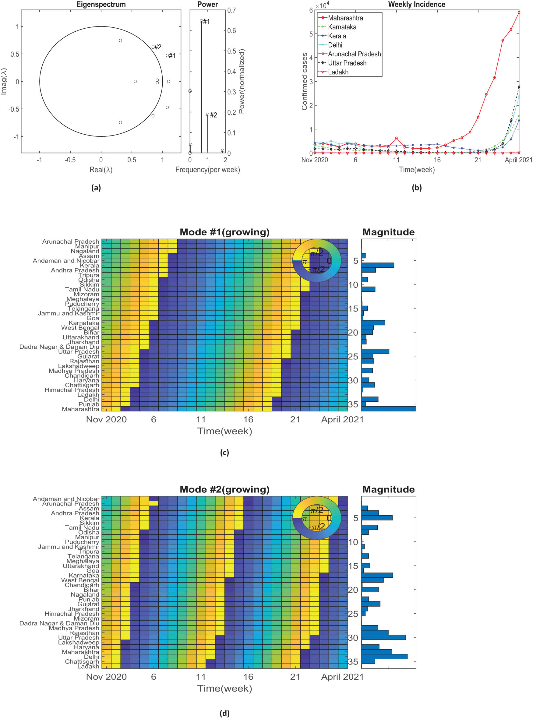
The second window at rank 10 truncation. (a) Left panel shows the discrete eigenspectrum plotted against a unit circle. Right panel shows the power vs frequency plot of the corresponding DMD modes. (b) Weekly incidence of COVID-19 cases from November 2020 to April 2021 for some selected states. Both # 1 and # 2 represents growing modes. (c and d) Left panel shows the time evolution of phase, and right panel shows magnitude of the # 1 and # 2 DMD mode.

For phase analysis, we are primarily interested in the complex eigenvalues since real ones do not have a phase. We chose DMD modes having the largest power corresponding to these complex eigenvalues represented by # 1 and # 2 in Figure 4(a). We observe that both of the selected/chosen DMD modes lie in the category of growing modes. These dominant DMD modes are then utilized to carry out phase analysis. We infer the phase difference to be the time lag (in weeks) between region-specific peaks of the COVID-19 outbreak.

The magnitude analysis demonstrates that Maharashtra, Delhi, Uttar Pradesh, Kerala, and Karnataka’s cumulative confirmed cases have a substantially large magnitude, which in fact complies with the data shown in Figure 4(c) and (d). The government critiqued the lax safety protocols and negligence by people during Diwali, Christmas, and New Year celebrations for the surge in cases. The spike in cases in Kerala has been attributed to violating protocols in political campaigns and house visits during local body elections in December 2020. Delhi, the capital city, witnessed a large-scale farmers’ protest, a nationwide strike by thousands of farmers at Delhi borders during the second wave, which caused an alarming rise in the number of COVID-19 cases. Uttar Pradesh, India’s most populated state, eased out restrictions during the village council elections [14] (Gram Panchayat Election 2021) held in April 2021. More than 1,600 teachers died of COVID who supervised those elections in the same month, as stated by a well-known teachers union. The second most populous state, Maharashtra, and the worst-hit state during the outbreak blamed complacency, poor masking, overcrowding, and scant guidelines about what should be open and what should be closed. Considering its high transmissibility, it is impossible to implement social-distancing rules without a complete lockdown in such crowded places as marine drive. Bengaluru, the epicenter of Karnataka, faced crowds at airports that were often seen without masks and violating other protocols like maintaining social distance in marriage halls, marketplaces, and malls.

Next, we discuss phase analysis from the two selected DMD modes. We state two observations:

1. In the DMD mode # 1 , the maximum phase difference is between Maharashtra and Arunachal Pradesh which is computed to be 3.39 weeks.

2. In the DMD mode # 2 , the maximum phase difference is between Arunachal Pradesh and Ladakh, which is evaluated to be 2.6 weeks.

3.3 The third window: April 2021 to October 2021

The third window also consists of 26 weeks, so the compatible spatial vs temporal resolution will be of order 36 × 26 . Figure 5(a) represents power of DMD modes, which will enable us to select the dominant DMD for carrying out magnitude and phase analysis. We selected top two DMD modes having largest power denoted by # 1 and # 2 . We observed that both the selected DMD modes correspond to decaying mode. We perform magnitude analysis by investigating the selected dominant modes. The mode # 1 analysis ascertains that Kerala has exceptionally high magnitude. Next in line, the magnitude of states like Maharashtra, Tamil Nadu, and Karnataka is also considerably high as illustrated in Figure 5(c) and (d). This rise may be attributed to millions of pilgrims at Kumbh Mela, which is celebrated after every 12 years and is the largest gathering of humanity on earth. This unique event, held in the month of April 2021, proved to be a super-spreader event for next consequent months. In particular, for Kerala, lack of active surveillance during Bakrid and onam celebrations during July and August made the situations worse.

Figure 5

The third window at rank 10 truncation. (a) Left panel shows the discrete eigenspectrum plotted against a unit circle. Right panel shows the power vs frequency plot of the corresponding DMD modes. Both # 1 and # 2 represents decaying modes. (b) Weekly incidence of COVID-19 cases from April 2021 to October 2021 for some selected states. (c and d) Left panel shows the time evolution of phase and right panel shows magnitude of the # 1 and # 2 DMD mode.

The phase analysis of mode # 1 provides us the fact that maximum phase difference is between Kerala and Nagaland whose value is 18.36 weeks, which is way more than the maximum phase difference evaluated in second window. The maximum phase difference in mode # 2 is between Assam and Kerala, which is computed to be 7.03 weeks. Investigating mode # 1 , we discover that phases of Haryana, Punjab, and Rajasthan are similar, and they are all located in the northern part of India sharing borders. The analysis suggests that there is strong connection with the spatial location of states in the third wave. But, we notice that there exist states having independent phase behavior, not affected by phase structure of states close to them spatially. In mode # 2 , we see that Assam and Arunachal Pradesh have independent phase behavior despite sharing borders with each other.

3.4 Reconstruction of district and statewise data

In this subsection, we have used Dataset A for the reconstruction of district vs date data (cumulative cases). The reconstructed data of top 20 districts with most COVID cases have been visualized in Figure 6. DMD has been applied to this dataset and the truncation of rank 530 has been chosen in order to construct the new data. We have plotted the reconstructed data obtained from equation (8) with black bold line, and the red dots indicate the original data points spaced equidistantly. DMD has performed extremely well in the reconstruction, which can also be verified by the error analysis done in Section 3.5. In addition to this, we have reconstructed state vs week (cumulative cases) data using CwDMD. Rank 34, 10, and 8 truncation have been chosen for window first, second, and third, respectively.

Figure 6

(a) In each panel, red dots show the daily cases data and bold line indicates the reconstructed data for each district. (b) In each panel, red dots show the weekly cases data and bold line indicates the reconstructed data for each state.

3.5 Error analysis

To ensure the accuracy and reliability of the results, it is important to perform proper error analysis. Error analysis in DMD involves assessing the quality of the reconstructed data and comparing it to the original data. One common approach to error analysis in CwDMD and DMD is to use a measure of the discrepancy between the original data and the reconstructed data, for which we use the relative error. Relative error is the ratio of the normed error to the norm of the original data.

The top panel in Figure 7 shows the error comparison of CwDMD and DMD in the reconstruction of dataset B. Note that this dataset is incompatible for DMD architecture, as spatial resolution is less than temporal resolution, which can be verified in the figure. We performed SVD with rank 34 truncation, resulting in huge errors because of the inconsistent data. Using CwDMD on same dataset, the reduction in error is significant, showing the importance of CwDMD. The dataset has been divided into three compatible windows with each window having resolution 36 × 26 . We performed SVD with rank 24, 10, and 8 truncation in window 3.1, 3.2, and 3.3, respectively, which resulted in comparatively less error as produced from DMD. When the data are inconsistent, CwDMD has an upper hand over the classical DMD and its variants. It is generally because we have more control over the system, in the sense that, we can choose the resolution of windows as per our requirement and can choose different rank r truncation for each window.

Figure 7

Top panel shows the relative error in the reconstruction of dataset B using DMD and CwDMD. Bottom panel shows the relative error in the reconstruction of dataset A using DMD.

In the below panel we have applied DMD on dataset A, with rank 530 truncation. It can be noted that DMD works remarkably well when the data is consistent. The reconstructed data in this panel have produced very less error.

References

[1] Andrews, M., Areekal, B., Rajesh, K., Krishnan, J., Suryakala, R., Krishnan, B., … Santhosh, P. (2020). First confirmed case of COVID-19 infection in India: A case report. The Indian Journal of Medical Research, 151(5), 490. 10.4103/ijmr.IJMR_2131_20Suche in Google Scholar PubMed PubMed Central
[2] Babu, J., Shukla, A., & Bharath. India’s COVID-19 districtwise data. https://github.com/covid19india/data/tree/gh-pages. Accessed: November 2022. Suche in Google Scholar
[3] Banaji, M. (2021). Estimating COVID-19 infection fatality rate in Mumbai during 2020. medRxiv, (p. 2021–04). 10.1101/2021.04.08.21255101Suche in Google Scholar
[4] Bistrian, D., Dimitriu, G., & Navon, I. (2019). Processing epidemiological data using dynamic mode decomposition method. AIP Conference Proceedings, 2164, 080002, AIP Publishing LLC. 10.1063/1.5130825Suche in Google Scholar
[5] Bistrian, D. A., Dimitriu, G., & Navon, I. M. (2020). Application of deterministic and randomized dynamic mode decomposition in epidemiology and fluid dynamics. Annals of the Alexandru Ioan Cuza University-Mathematics, 66(2), 251–287. Suche in Google Scholar
[6] Bistrian, D. A., Dimitriu, G., & Navon, I. M. (2020). Modeling dynamic patterns from COVID-19 data using randomized dynamic mode decomposition in predictive mode and ARIMA. AIP Conference Proceedings, 2302(1), 080002. 10.1063/5.0033963Suche in Google Scholar
[7] Dhamodharavadhani, S., Rathipriya, R., & Chatterjee, J. M. (2020). COVID-19 mortality rate prediction for India using statistical neural network models. Frontiers in Public Health, 8, p. 44110.3389/fpubh.2020.00441Suche in Google Scholar PubMed PubMed Central
[8] Duke, D., Soria, J., & Honnery, D. (2012). An error analysis of the dynamic mode decomposition. Experiments in Fluids, 52, 529–542. 10.1007/s00348-011-1235-7Suche in Google Scholar
[9] Gupta, A. K., Singh, V., Mathur, P., & Travieso-Gonzalez, C. M. (2021). Prediction of COVID-19 pandemic measuring criteria using support vector machine, prophet and linear regression models in Indian scenario. Journal of Interdisciplinary Mathematics, 24(1), 89–108. 10.1080/09720502.2020.1833458Suche in Google Scholar
[10] Kim, S., Kim, M., Lee, S., & Lee, Y. J. (2021). Discovering spatiotemporal patterns of COVID-19 pandemic in South Korea. Scientific Reports, 11(1), 24470. 10.1038/s41598-021-03487-2Suche in Google Scholar PubMed PubMed Central
[11] Kumar, S., Sharma, S., Singh, F., Bhatnagar, P., & Kumari, N. (2021). A mathematical model for COVID-19 in Italy with possible control strategies. In N. H. Shah & M. Mittal, (Eds.), Mathematical Analysis for Transmission of COVID-19, (pp. 101–124), Singapore: Springer. 10.1007/978-981-33-6264-2_6Suche in Google Scholar
[12] Kumar, V. M., Pandi-Perumal, S. R., Trakht, I., & Thyagarajan, S. P. (2021). Strategy for COVID-19 vaccination in India: The country with the second highest population and number of cases. NPJ Vaccines, 6(1), 60. 10.1038/s41541-021-00327-2Suche in Google Scholar PubMed PubMed Central
[13] Kutz, J. N., Brunton, S. L., Brunton, B. W., & Proctor, J. L. (2016). Dynamic mode decomposition: Data-driven modeling of complex systems. SIAM. 10.1137/1.9781611974508Suche in Google Scholar
[14] Mahmood, Z. (2022). Elections During Covid-19: The Indian Experience in 2020–2021. Case Study, Stockholm: International Institute for Democracy and Electoral Assistance. Suche in Google Scholar
[15] Malavika, B., Marimuthu, S., Joy, M., Nadaraj, A., Asirvatham, E. S., & Jeyaseelan, L. (2021). Forecasting COVID-19 epidemic in India and high incidence states using SIR and logistic growth models. Clinical Epidemiology and Global Health, 9, 26–33. 10.1016/j.cegh.2020.06.006Suche in Google Scholar PubMed PubMed Central
[16] Mathieu, E., Ritchie, H., Rodés-Guirao, L., Appel, C., Giattino, C., Hasell, J., … Roser, M. (2020). Coronavirus Pandemic (COVID-19). Our World in Data. https://ourworldindata.org/coronavirus. Suche in Google Scholar
[17] Ministry of Health and Family Welfare. Population projection report. https://main.mohfw.gov.in/reports-0, Accessed: February 2023. Suche in Google Scholar
[18] National Portal of India. India at a glance. https://www.india.gov.in/india-glance/states-india. Accessed: February 2023. Suche in Google Scholar
[19] Proctor, J. L., & Eckhoff, P. A. (2015). Discovering dynamic patterns from infectious disease data using dynamic mode decomposition. International Health, 7(2), 139–145. 10.1093/inthealth/ihv009Suche in Google Scholar PubMed PubMed Central
[20] Quadri, S. A., & Padala, P. R. (2021). An aspect of Kumbh Mela massive gathering and COVID-19. Current Tropical Medicine Reports, 8, 225–230. 10.1007/s40475-021-00238-1Suche in Google Scholar PubMed PubMed Central
[21] Rocha, I. C. N., Pelayo, M. G. A., & Rackimuthu, S. (2021). Kumbh Mela religious gathering as a massive superspreading event: Potential culprit for the exponential surge of COVID-19 cases in India. The American Journal of Tropical Medicine and Hygiene, 105(4), 868. 10.4269/ajtmh.21-0601Suche in Google Scholar PubMed PubMed Central
[22] Roy, S., Bhunia, G. S., & Shit, P. K. (2021). Spatial prediction of COVID-19 epidemic using ARIMA techniques in India. Modeling Earth Systems and Environment, 7, 1385–1391. 10.1007/s40808-020-00890-ySuche in Google Scholar PubMed PubMed Central
[23] Schmid, P. J. (2010). Dynamic mode decomposition of numerical and experimental data. Journal of Fluid Mechanics, 656, 5–28. 10.1017/S0022112010001217Suche in Google Scholar
[24] The Lancet. (2020). India under COVID-19 lockdown. The Lancet, 395(10233), 1315. 10.1016/S0140-6736(20)30938-7Suche in Google Scholar PubMed PubMed Central
[25] Tu, J. H. (2013). Dynamic mode decomposition: Theory and applications. (PhD thesis). Princeton, NJ, USA: Princeton University. Suche in Google Scholar
[26] Viguerie, A., Barros, G. F., Grave, M., Reali, A., & Coutinho, A. L. (2022). Coupled and uncoupled dynamic mode decomposition in multi-compartmental systems with applications to epidemiological and additive manufacturing problems. Computer Methods in Applied Mechanics and Engineering, 391, 114600. 10.1016/j.cma.2022.114600Suche in Google Scholar
© 2023 the author(s), published by De Gruyter
This work is licensed under the Creative Commons Attribution 4.0 International License.
Artikel in diesem Heft
- Special Issue: Infectious Disease Modeling In the Era of Post COVID-19
- A comprehensive and detailed within-host modeling study involving crucial biomarkers and optimal drug regimen for type I Lepra reaction: A deterministic approach