Experimental measurement and numerical predictions of thickness variation and transverse stresses in a concrete ring

1 Introduction

A particular concern related to the design of thick concrete shells is the control of cracking, deflection, buckling, and dimensional variations among others. Steel bars or fiber reinforcements are more often incorporated in the concrete in order to limit cracking, especially in restrained conditions [1]. Concerning displacements, several calculating methods are proposed in the literature, including analytical methods for simple shapes and simple shell models [2]. To this end, the literature presents two main approaches to shell modeling, namely, three-dimensional (3D) models and two-dimensional (2D) models.

For 2D models, several authors [3,4,5,6] calculate the displacements by using classical theories due to Love, Sander, and Kirchhoff, where the proposed kinematics satisfy the Kirchhoff–Love hypotheses, i.e., normal segments to the mid-surface before deformation remain rigid and normal to the deformed mid-surface ( ε x z = ε y z = 0 ) . So, transverse strains do not contribute to the strain energy. Also, transverse shear stress σ α 3 and the pinch stress σ 33 are neglected. Nevertheless, according to Fantuzzi et al. [7], the generalized differential quadrature finite element method theory presents a good agreement with the calculated deflection. Some authors use this method to solve several complex engineering problems including doubly curved anisotropic shells with variable thickness [8,9,10], non-uniform rational basis spline [10], circular/elliptical cylindrical shells, and beam structures [11]. The governing equations of the problem are obtained by using the Hamiltonian principle. Later, the strong finite element method based on differential quadrature proposed by Tornabene et al. [12] improved the quality of results obtained with the classical finite element method. This theory has proven efficiency on composite shells. The N-T theory proposed by Nzengwa and Tagne [13] introduced the Gauss deformation strain tensor and calculated the transverse stress σ i 3 as reactions to a more general plane strain. In previous studies [14,15], based on this approach, a family of finite elements (CSFE and CSFE-sh) was implemented. Numerical results were compared to the existing reference benchmarks with satisfaction. In previous studies [16,17], a higher order trigonometric, exponential, or polynomial expansion series is used to approximate the displacement with greater precision. However, boundary conditions become very complex and difficult to be satisfied by higher order terms.

Unlike 2D models, 3D models have the advantage of avoiding complex shell finite elements. Because the 3D constitutive law is used, thickness variation and large rotations are well addressed since displacements are the only degrees of freedom [18]. However, locking phenomena are encountered during computation especially when the shells become thin [19]. To overcome the locking phenomenon, recent works have proposed hexahedral finite elements named SHB15 and SHB20 [20,21]. Researchers [22,23,24,25,26,27] in this field propose a hybrid formulation for thickness rectification and stress calculation. Although many advantages exist, this approach remains memory greedy and requires much longer computation time. A development of simplified 3D approaches, which reduce calculating time, is necessary. Other models of thick shells due to Hencky, Timoshenko–Mindlin, Naghdi–Berry, and Reissner–Mindlin, which are 2D models, have reduced the number of nodes but do not account for the variation of thickness [28]. Nzengwa’s approach (the N model) calculates transverse stresses [28] and the variation of thickness [29]. In the study by Fantuzzi et al. [7], a general displacement field based on a unified formulation [17] including the stretching and zig-zag effects is proposed by using higher order expansion field.

The aim of this study was to investigate the effects due to mechanical loading on thickness variation ( Δ h ) , displacement ( u 3 ) , and the total stresses and strains ( σ i j , ε i j ) through the thickness.

The first section of this work is the introduction. Some previous models are presented with their achievements. Their strong and weak points are mentioned. Section 2 is devoted to the description of the model under investigation. The kinematics and the resulting variational equations to be implemented are addressed. The finite element is described. In Section 3, we describe the experimental device. In Section 4, the numerical and experimental data are presented in tables and curves and compared. The performance of the model is discussed.

2 Application of the model on a ring

The model proposed by Nzengwa [29] is a 2D 4-parameter model based on a kinematic derived from a differential equation, described as follows:

Let ϕ ( x 1 , x 2 , z ) = ( ϕ i ) be such that ϕ α ( x , z ) = ε α 3 + ε 3 α = 2 ε α 3 , ϕ 3 ( x , z ) = ε 33 . We suppose rot ( ϕ ) = 0 rot ( ϕ ) i = ϕ i + 1 , i + 2 − ϕ i + 2 , i + 1 mod [3].

The solution of this equation is the kinematic

where U α ( x , z ) and U 3 ( x , z ) are components of the displacement in the shell’s contravariant base; { g α = ( μ − 1 ) ρ α a ρ , g 3 = a 3 } and { a 3 = a 3 } are contravariant bases of the mid-surface; g α = μ α ρ a ρ = ( δ α ρ − z B α ρ ) a ρ and { a ρ , a 3 } are covariant bases of the shell and its mid-surface, respectively; ψ = det ( μ α ρ ) , u α ( x ) , and u 3 ( x ) are functions defined on the mid-surface; B α ρ is the mixed component of the curvature tensor; B ρ α is the covariant component of the curvature tensor; δ α ρ is Kronecker’s symbol on the mid-surface.

where ε 33 = w ′ ( z ) q ¯ ( x ) , ε α z = 1 2 ∂ α q , q = w ( z ) q ¯ ( x ) , and γ α β ( x ) = − 1 2 ( μ α ρ B ρ β + μ β ρ B ρ α ) are the section warping tensors.

The membrane strain tensor or change of the first fundamental form is

Γ ¯ β α ρ Christoffel symbol on the mid-surface is

The curvature deformation tensor or change of the second fundamental form is

The Gauss deformation tensor or change of the third fundamental form is

w ( z ) : the transverse stretching distribution function.

We consider a regular mesh (Figure 1) with a physical parameterization ( x , R θ ) = ( x 1 , x 2 ) ; then, the mid-surface base is

Figure 1

Triangular shell element.

Using Eq. (2), we have

The constitutive law reads

g i j = g i . g j , g i j = g i . g j , a α β = a α ⋅ a β , a α β = a α ⋅ a β are the contravariant and covariant components of the metric tensors of the shell and mid-surface, respectively, while λ ¯ , μ ¯ are the Lamé elastic moduli. Young’s modulus and Poisson’s coefficient E , v ¯ can also be used. The boundary value problem consists to find

with

U ad = ( H γ 0 1 ( S ) × H 1 ( S ) × H 2 ( S ) × H 1 ( S ) ) , H γ 0 1 ( S ) = { u ∈ H 1 ( S ) , u = 0 on γ 0 } , H m ( S ) = { u ∈ L 2 ( S ) ; ∂ α u ∈ L 2 ( S ) , α = ( α 1 , α 2 ) , ∣ α ∣ ≤ m } , L 2 ( S ) is the set of square-integrable functions defined on the mid-surface, and γ 0 is a portion of the boundary of the mid-surface where the displacement is fixed.

Let A α β δ τ = λ ¯ g α β g δ τ + 2 μ ¯ g α τ g τ β .

Then,

We also define

Then, for the best first order, G α β ≈ a α β , ψ ≈ 1 , the variational equation reads

where

where P ¯ 4 = ∫ h 2 − h 2 f 3 w d z + w h 2 p ¯ + 3 − w − h 2 p ¯ − 3 , θ ¯ α ( v ) = − ( ∂ α v 3 + B α ρ v ρ ) is the virtual angle of rotation of a cross section at the free border of the mid-surface in the direction of the base vector a α .

We use iso-parametric Lagrangian symplectic-type triangle finite elements, which are based on complete polynomial bases. The finite element used has four degrees of freedom at the vertex nodes (three displacements and one stretching) and one degree of freedom at mid-points of edges (one for the transverse displacement). So, shape functions for the membrane displacements are linear, while the transverse displacement is quadratic. The matrix of shape functions is defined as follows:

3 Experimental device

In this study, two series of thin and thick concrete ring specimens were casted and instrumented for strains and thickness variation monitoring during the loading test. Concrete wall thicknesses of 6.8 and 12 cm referred to as “thin rings” and “thick rings,” respectively, were casted and covered with a plastic film. The ring specimens were demolded 28 days after casting. The geometric and mechanical parameters are presented in Table 1. The width of the rings was kept constant at 15 cm. The shapes and descriptions of the geometries considered are shown in Figure 2. The uniaxial compressive strength of concrete was determined on the cubic specimens of 10 cm side at 28 days. The average compressive strength (fc) of concrete obtained on six specimens was fc = 43.86 MPa.

Figure 2

Geometry details of test specimen.

The instrumented ring specimens and data acquisition system used are shown in Figure 3. We considered:

1. Two concrete rings according to the value of the characteristic ratio χ for “thin rings” or “thick rings” configuration test;

2. A car inflatable wheel for radial pressure loading;

3. The micrometer-sensitive digital comparators for displacement measurement. The value retained is the average of the measurements recorded on the three comparators;

4. Two strain gauges are glued to the outer sheet of each ring for strain monitoring. The value retained is the average of the measurements recorded on the two strain gauges;

5. A data acquisition system in a quarter-bridge configuration for strain recording.

Figure 3

Description of experimental device and details of data acquisition units.

4 Results and discussion

4.1 Validation of the model

4.1.1 Convergence test

According to the classical theory of linear elasticity for a cylindrical shell under uniform internal pressure, the analytical expression for radial displacement is expressed as follows [2]:

(18) U r = 1 E ceff r r i 2 P i r e 2 − r i 2 ( 1 − v ) + ( 1 + v ) r e 2 r 2

with E ceff = E 1 + φ ( t 0 ) ,

where r is the mid-surface’s radius of the ring, r _e is the outer radius, r _i is the inner radius, and P _i the radial pressure. The test is done on a thick ring. The parameters used are those recorded in Table 1.

The analytical solution obtained for the concrete ring in the configuration of “thick shell” is equal to 54.75 µm.

Figure 4 shows the evolution of radial displacement from a point at the mid-surface obtained with the model under radial loading. The ring is blocked in the lower base so that the displacements in the x-direction are zero. The numerical solution gives good results by refining the mesh. It can be observed that with a mesh corresponding to 224 elements, we have a relative error of 0.86% between analytical and numerical solutions. This shows a good numerical prediction (Table 2).

Figure 4

Mid-surface displacement–convergence test.

Table 2

Evolution of mid-surface displacement – numerical and analytical comparison

Mesh	Nber_of elements	U_analytic (µm)	U_num (µm)	Relative error (%)
2 × 4 × 3	24	54.75	73.04	33.39
3 × 4 × 4	48	54.75	65.33	19.31
4 × 4 × 5	80	54.75	59.8	9.21
5 × 4 × 6	120	54.75	57.44	4.90
6 × 4 × 7	168	54.75	55.77	1.85
7 × 4 × 8	224	54.75	55.23	0.86

4.1.2 Evolution of radial displacements

The results of radial displacements simulated at mid-surface of the two types of rings and experimental results are presented in Figure 5. One can observe that the shape of the curves globally shows an increase in displacement with pressure, especially for pressure values greater than two bars. For the values of pressures lower than two bars, the displacements are rather weak for the thin ring and almost null for the thick ring. This behavior is probably due to the fact that for low-pressure values, a large part of energy is absorbed by the saturated sand membrane, which is undoubtedly in its consolidation phase. Another reason may be due to the fact that concrete is a material with a nonlinear behavior. The observed value difference may be due to the complex behavior of the concrete ring.

Figure 5

Evolution of radial displacement of the mid-surface according to the load.

The sensitivity of the comparators used and the accessories probably do not allow very small dimensional changes to be detected.

Finally, for pressure values greater than two bars, the curves of the simulations are quite close to the experimental results with the relative error close to 11% for the two configurations as presented in Table 3.

Table 3

Relative error between experimental results and numerical calculation for radial displacement investigation

Pressure (bar)	χ = 0.1007			χ = 0.1667
	Experimental displacement (µm)	Numerical displacement (µm)	Relative error (%)	Experimental displacement (µm)	Numerical displacement (µm)	Relative error (%)
0.5	2.93	12.72	77.00	—	—	—
1	6.58	25.45	74.13	0	9.27	100
1.5	23.41	38.17	38.69	0	13.91	100
2	41.69	50.90	18.09	11	18.55	40.70
2.5	52.66	63.62	17.22	15	23.188	35.31
3	69.48	76.35	9.00	22	27.82	20.92
3.5	80.46	89.07	9.67	29	32.46	10.66
4	91.43	101.80	10.19	36	37.1	2.96
4.5	101.67	114.53	11.23	40	41.73	4.15
5	117.76	127.25	7.46	43	46.38	7.29
5.5	—	—	—	46	51.01	9.82
6	—	—	—	58	55.65	4.22
6.5	—	—	—	61	60.28	1.19

The displacement curves obtained by numerical simulation are perfectly linear. The value of the displacement evolves with the load in accordance with the linear shell model used.

4.1.3 Evolution of the hoop strains in the thick ring

The results of the hoop strains simulated at the external surface for the thick ring and those experimental are presented in Figure 6. One can observe that both measured strains and those simulated evolve in the same way with the same amplitude and similar kinetic evolution. Also, the shape of the curves globally shows an increase in strains with pressure. The curves of the simulations are quite close to the experimental results and this is for the two rings, with an average of relative error close to 20% for thick rings as presented in Table 4.

Figure 6

Evolution of strain in the hoop (ε ₂₂) as a function of the load (χ = 0.1667).

Table 4

Relative error between experimental values and model predictions for hoop strains

Pressure (bar)	Thick ring (χ = 0.1667)
	Experimental mean strains (µm/m)	Numerical strains (µm/m)	Relative error (%)
0.5	1.25	2.52	50.36
1	2.25	3.78	40.43
1.5	3.375	5.04	32.99
2	4.5	6.30	28.52
2.5	6.25	7.55	17.27
3	8	8.81	9.23
3.5	9.5	10.07	5.69
4	11	11.33	2.93
4.5	13.5	12.59	7.22
5	15.25	13.85	10.11
5.5	17.5	15.11	15.82
6	19.75	16.37	20.66

Let us notice that beyond five bars, the experimental strains are higher than that of the model, which can be attributed to the predominance of the nonlinear behavior at this phase (Figure 7).

Figure 7

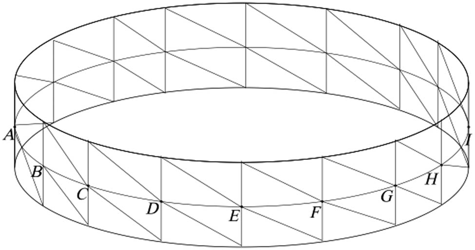
Mesh of the ring.

4.1.4 Variation of thickness

Figure 8 presents the variation of thickness due to pressure loading and the evolution of the resulting strains in the thickness. One can see that the model is able to reproduce the experimental measurements of thickness variation for both configurations. In the same way, the average values of relative errors of thickness variation between simulated and experimental campaigns are close to 19% for thin rings and 27% for thick rings as presented in Table 5. The observed value difference may be attributed to both the nonlinear behavior of the concrete and the sensitivity of the digital comparators.

Figure 8

Evolution of thickness variation.

Table 5

Relative error between experimental and model predictions for thickness variation

Pressure (bar)	χ = 0.1007			χ = 0.1667
	Experimental thickness (µm)	Numerical thickness (µm)	Relative error (%)	Experimental thickness (µm)	Numerical thickness (µm)	Relative error (%)
0	0	0	—	0	0	—
1	1	2.1	52.38	0.65	0.6	8.33
2	3.2	4.1	21.95	2	1.2	66.67
3	4.95	6.2	20.16	2.5	1.8	38.89
4	7.15	8.2	12.80	3.05	2.4	27.08
5	9.6	10.3	6.80	3.75	3	25.00
6				4.5	3.6	25.00

Figure 9 shows the different values obtained depending on whether we are in a thin (Figure 9a) or thick (Figure 9b) shell of the new thickness in micrometers under radial mechanical loading. The pressure values are recorded in the legend. The calculation of the new thickness is done by means of the fourth parameter of the “N” elastic shell model proposed by Nzengwa [29].

Figure 9

(a) Thickness evolution in the thin ring. (b) Thickness evolution in the thick ring.

4.2 Stress and strain computation in the thickness of the ring

A finite element analysis of the concrete rings based on the elastic shell model proposed by Nzengwa [29] was carried out. The stress and strain variations through the thickness for both thin and thick concrete rings are plotted at a particular point A on the mid-surface as presented in Figures 9 and 10. They show the evolution of stresses on the inner and outer sheets of rings in loading conditions.

Figure 10

(a) Stress- σ 11 z = − h 2 , z = h 2 , (b) stress- σ 22 z = − h 2 , z = h 2 , (c) stress- σ 33 z = − h 2 , z = h 2 , (d) stress- σ 12 z = − h 2 , z = h 2 , (e) stress- σ 13 z = − h 2 , z = h 2 , and (f) stress- σ 23 z = − h 2 , z = h 2 .

In the case of the thin shell, the stresses increase with the pressure loading. One can see clearly the difference of stresses between inner sheet and outer sheet when pressure increases. Generally, the stress in the outer sheet is greater than that of the inner sheet and this difference increases with pressure.

With the increase in the thickness of concrete specimens (thick rings), the stresses increase with the pressure loading. Generally, the stress plotted in the outer sheet is greater than that of the inner sheet and this difference increases with pressure. In comparison with thin rings, the computational stresses are low.

The low distortion values for the pressure simulation justify the fact that the shears are almost zero. As for the distortions on inner and outer sheets, a symmetry with respect to the x-axis is observed. We can also mark this symmetrical look of the works of Gruttmann and Wagner [30] where the authors present the stresses according to the thickness for the case of a square sandwich plate with a layup.

5 Conclusion

In this study, experimental and numerical investigations were performed on the concrete rings. The shell model (the N model or Nzengwa’s model) used allows us to follow the evolution of the stresses in the thickness as well as the variation of section. The main results are as follows:

1. The calculation of displacements in each of the two configurations according to the loading gives linear curves. In addition, these results are close to the values measured (Figure 5);

2. Subsequently, we computed and measured the hoop deformation ε ₂₂ (outer sheet) and the mean relative error between experimentation and computation is around 20% (Figure 6). The model is able to determine the transverse stresses and transverse strains as shown in Figures 10a–f and 11a–f, respectively;

3. Finally, we present the superposition of the curves of the thickness variation calculated and measured, as a function of the load (Figure 8).

Figure 11

(a) strain- ε 11 z = − h 2 , z = h 2 , (b) strain- ε 22 z = − h 2 , z = h 2 , (c) strain- ε 33 z = − h 2 , z = h 2 , (d) strain- ε 12 z = − h 2 , z = h 2 , (e) strain- ε 13 z = − h 2 , z = h 2 , and (f) strain- ε 23 z = − h 2 , z = h 2 .

Displacement determination, transverse stresses, and thickness variation are possible because of the stretching parameter q ( x , z ) = w ( z ) q ¯ ( x ) . The simulation results presented in this study are obtained for a polynomial function w ( z ) ; i.e., only the first-order term of the Taylor expansion of the stretching parameter is considered. Note that the choice of a polynomial of higher degree or another form of the distribution w ( z ) could improve the quality of the results. Finally, we were able to present different loadings of the variation of the thickness of the ring. In addition, it is clear that the model gives satisfactory results in thin and thick shells.

References

[1] Chang Z-T, Bradford MA, Gilbert RI. Short-term behaviour of shallow thin-walled concrete dome under uniform external pressure. Thin-Walled Struct. 2011;49:112–20.10.1016/j.tws.2010.08.012Search in Google Scholar
[2] Hojjati MH, Hossaini A. Theoretical and numerical analyses of rotating discs of non-uniform thickness and density. Int J Press Vessel Pip. 2008;85(10):694–700.10.1016/j.ijpvp.2008.02.010Search in Google Scholar
[3] Novozhilov VV. The theory of thin elastic shells. Vol. 164. Moscow: Norodhoff; 1964.10.1007/978-94-017-5352-4Search in Google Scholar
[4] Love AEH. The small free vibrations and deformation of a thin elastic shells. Phil Trans Roy Soc London, (Ser A 179). 1888;179:491–546.10.1098/rsta.1888.0016Search in Google Scholar
[5] Kirchhoff G. Über das Gleichgewicht und die Bewegung einer elastischen scheibe. J für Reine Angew Math. 1850;40:51–88.10.1515/crll.1850.40.51Search in Google Scholar
[6] Leissa AW. Vibration of shells. Washington, D.C: NASA; 1973.Search in Google Scholar
[7] Fantuzzi N, Tornabene F, Viola E. Generalized differential quadrature finite element method for vibration analysis of arbitrarily shaped membranes. Int J Mech Sci. 2013;79:216–51.10.1016/j.ijmecsci.2013.12.008Search in Google Scholar
[8] Tornabene F, Viscoti M, Dimitri R, Reddy JN. Higher order theories for the vibration study of doubly-curved anisotropic shells with a variable thickness and isogeometric mapped geometry. Compos Struct. 2021;267:113829.10.1016/j.compstruct.2021.113829Search in Google Scholar
[9] Tornabene F, Viscoti M, Dimitri R. Equivalent single layer higher order theory based on a weak formulation for the dynamic analysis of anisotropic doubly-curved shells with arbitrary geometry and variable thickness. Thin-Walled Struct. 2022;174:109119.10.1016/j.tws.2022.109119Search in Google Scholar
[10] Tornabene F, Viscoti M, Dimitri R. Static analysis of anisotropic doubly-curved shells with arbitrary geometry and variable thickness resting on a Winkler-Pasternak support and subjected to general loads. Eng Anal Bound Elem. 2022;140:618–73.10.1016/j.enganabound.2022.02.021Search in Google Scholar
[11] Fazzolari FA, Viscoti M, Dimitri R, Tornabene F. 1D-Hierarchical Ritz and 2D-GDQ Formulations for the free vibration analysis of circular/elliptical cylindrical shells and beam structures. Compos Struct. 2021;258:113338.10.1016/j.compstruct.2020.113338Search in Google Scholar
[12] Tornabene F, Fantuzzi N, Ubertini F, Viola E. Strong formulation finite element method based on differential quadrature: a survey. Appl Mech Rev. 2015;67(2):55.10.1115/1.4028859Search in Google Scholar
[13] Nzengwa R, Tagne SBH. A two-dimensional model for linear elastic thick shells. Int J Solids Struct. 1999;136:5141–76.10.1016/S0020-7683(98)00165-6Search in Google Scholar
[14] Nkongho AJ, Nzengwa R, Amba JC, Ngayihi ACV. Approximation of linear elastic shells by curved triangular finite elements based on elastic thick shells theory. Math Probl Eng. 2016;2016:1–12.10.1155/2016/8936075Search in Google Scholar
[15] Nkongho J, Amba JC, Essola D, Ngayihi A, Bodol M, Nzengwa R. Generalised assumed strain curved shell finite elements (CSFE-sh) with shifted-Lagrange and application on N-T’s shells theory. Curved Layer Struct. 2020;7(1):125–30.10.1515/cls-2020-0010Search in Google Scholar
[16] Murakami H. Laminated composite plate theory with improved in-plane responses. J Appl Mech. 1986;53:661–6.10.1115/1.3171828Search in Google Scholar
[17] Carrera E, Valvano S, Filippi M. Classical, higher-order, zig-zag and variable kinematic shell elements for the analysis of composite multilayered structures. Eur J Mech. 2018;72:97–110.10.1016/j.euromechsol.2018.04.015Search in Google Scholar
[18] Trinh VD, Abed-M F, Combescure A. A New assumed strain solid–shell formulation “SHB6” for the six-node prismatic finite element. J Mech Sci Technol. 2011;25(9):2345–64.10.1007/s12206-011-0710-7Search in Google Scholar
[19] Stolarsky H, Belytschko T. Membrane locking and reduced integration for curved elements. J Appl Mech. 1982;49:172–6.10.1115/1.3161961Search in Google Scholar
[20] Abed-M F, Combescure A. SHB8PS - a new adaptive, assumed-strain continuum mechanics shell element for impact analysis. Comput Struct. 2002;80:791–803.10.1016/S0045-7949(02)00047-0Search in Google Scholar
[21] Abed-M F, Combescure A. An improved assumed strain solid–shell element formulation with physical stabilization for geometric nonlinear applications and elastic plastic. stability analysis. Int J Num Methods Eng. 2009;80:1640–86.10.1002/nme.2676Search in Google Scholar
[22] Sze KY, Yao LQ. A hybrid stress ANS solid–shell element and its generalization for smart structure modelling. Part I- solid–shell element formulation. Int J Numer Methods Eng. 2000;48:545–64.10.1002/(SICI)1097-0207(20000610)48:4<545::AID-NME889>3.0.CO;2-6Search in Google Scholar
[23] Vu-Quoc L, Tan XG. Optimal solid shells for non-linear analyses of multilayer composites. I. Statics. Comput Methods Appl Mech Eng. 2003;192:975–1016.10.1016/S0045-7825(02)00435-8Search in Google Scholar
[24] Chen YI, Wu GY. A mixed 8-node hexahedral element based on the Hu–Washizu principle and the field extrapolation technique. Struct Eng Mech. 2004;17:113–40.10.12989/sem.2004.17.1.113Search in Google Scholar
[25] Kim KD, Liu GZ, Han SC. A resultant 8-node solid–shell element for geometrically nonlinear analysis. Comput Mech. 2005;35:315–31.10.1007/s00466-004-0606-9Search in Google Scholar
[26] Reese S. A large deformation solid–shell concept based on reduced integration with hourglass stabilization. Int J Numer Methods Eng. 2007;69:1671–1716.10.1002/nme.1827Search in Google Scholar
[27] Pian TH, Sze KY. Hybrid stress finite element methods for plate and shell structures. Adv Struct Eng. 2001;4:13–8.10.1260/1369433011502309Search in Google Scholar
[28] Mindlin RD. Influence of rotatory inertia and shear on flexural motions of isotropic, elastic plate. J Appl Mech. 1951;18:31–8.10.1007/978-1-4613-8865-4_29Search in Google Scholar
[29] Nzengwa R. A 2D model for dynamics of linear elastic thick shells with Transversal strains variation. In: Awrejcewicz J, editor. Proceedings of the 8th Conference on Dynamical Systems Theory and Applications. 2005 Dec 12–15; Lodz, Poland. Technical University of Lodz, 2005. p. 769–76.Search in Google Scholar
[30] Gruttmann F, Wagner W. An advanced shell model for the analysis of geometrical and material nonlinear shells. Comput Mech. 2020;66:1353–76.10.1007/s00466-020-01905-2Search in Google Scholar
© 2023 the author(s), published by De Gruyter
This work is licensed under the Creative Commons Attribution 4.0 International License.
Articles in the same Issue
- Research Articles
- Investigation of differential shrinkage stresses in a revolution shell structure due to the evolving parameters of concrete
- Multiphysics analysis for fluid–structure interaction of blood biological flow inside three-dimensional artery
- MD-based study on the deformation process of engineered Ni–Al core–shell nanowires: Toward an understanding underlying deformation mechanisms