Computing N-dimensional polytrope via power series

Mohamed I. Nouh; Mahmoud Taha; Ahmed Ahmed Ibrahim; Mohamed Abdel-Sabour

doi:10.1515/astro-2022-0230

Article Open Access

Computing N-dimensional polytrope via power series

Mohamed I. Nouh , Mahmoud Taha , Ahmed Ahmed Ibrahim and Mohamed Abdel-Sabour

Published/Copyright: April 12, 2024

Published by

Become an author with De Gruyter Brill

Submit Manuscript Author Information Explore this Subject

From the journal Open Astronomy Volume 33 Issue 1

Abstract

Polytropic equations (Lane–Emden [LE] equations) are valuable because they offer a simple explanation for a star’s interior structure, interstellar matter, molecular clouds, and even spiral arms that can be calculated and used to estimate various physical parameters. Many analytical and numerical methods are used to solve the polytropic LE equation. The series expansion method played an essential role in many areas of science and has found application in many branches of physical science. This work uses the series expansion method to examine N-dimensional polytropes (i.e., slab, cylinder, and sphere). To solve LE-type equations, a computational method based on accelerated series expansion (ASE) is applied. We calculate several models for the N-dimensional polytropes. The numerical results show good agreement between the ASE and numerical and analytical models of the N-dimensional polytropes.

Keywords: equation of state; N-dimensional polytrope; series solution; physical characteristic; stellar structure

1 Introduction

Polytropes are useful as they provide a simple solution for the internal structure of a star that can be tabulated and used for estimates of various quantities. They are much simpler to manipulate than the complete rigid solution of all the equations of stellar structure. This simplicity assumes a power relationship between the pressure and the density, which must hold throughout the star.

Over many decades, massive self-gravitating gas distributions have been observed in various locations around the galaxy, including the interstellar matter, molecular clouds, and even spiral arms (Chandrasekhar 1967, Kippenhahn et al., 2012, Maciel 2016).

These formations are roughly shaped like enormous flat sheets and long cylindrical threads. Consider endlessly vast planar polytropes with finite thicknesses or infinitely long cylindrical polytropes with finite radii as idealized models of such gas condensations (Horedt 2004).

A preliminary study on the Lane–Emden (LE) equations (polytropic and isothermal) was undertaken by Lane (1870) and Emden (1907). The LE-type equation, which simulates numerous occurrences in mathematical physics and astrophysics, is among the most fascinating. It is a nonlinear ordinary differential equation with a singularity at the origin that explains the equilibrium density distribution in the self-gravitating polytrophic isothermal gas sphere (Chandrasekhar 1967). This equation is of utmost significance in the study of radiative cooling and the modeling of galaxy clusters. The analysis of isothermal cores, convective stellar interiors, and degenerate stellar configurations have all shown them to be the most adaptable in various circumstances.

Besides numerical integration, there are many numerical solutions presented to solve LE equations, such as the genetic algorithm (e.g., Ge et al., 2008), lattice Boltzmann method (e.g., Zhang et al., 2003), ant colony algorithm (e.g., Cao and Guo 2011), artificial neural networks (e.g., Morawski and Bejger 2020), Monte Carlo methods by El-Essawy et al. (2023, 2024), optimal homotopy asymptotic method by Iqbal and Javed (2011), shifted Jacobi–Gauss collocation spectral method by Bhrawy and Alofi (2012), and new Galerkin operational matrices by Abd-Elhameed et al. (2016).

Approximate techniques exist to solve the LE problem outside numerical integration (Shawagfeh 1993). The first technique is to convert the equation into an integrodifferential equation before iterating it (Seidov 2000). Adomian et al. (1995) proposed the second approach. This approach derives the desired solution using Adomian’s decomposition method (Adomian 1983, Abdel-Salam et al., 2020) and then employs continued fractions to find an analytical approximation. Hunter (2001) and Nouh (2004) perform a series of solutions for the LE equations. For N-dimensional polytropes and the isothermal sphere, Saad (2004) develops literal analytical solutions to the LE equations; to increase the power series convergence’s physical range, he applies a specific alteration to the independent variable and Pade´ approximants. Series expansions of LE functions at an interior point of a polytrope with a generic geometric index N are shown by Horedt (1987).

In the present work, we study the structure of the N-dimensional polytope using power series. We construct a recurrence relation for the N-dimensional Lane–Emden (NLE) equation series solution. The Euler–Abel–Pade’ scheme (Nouh 2004) will accelerate the divergent series to obtain solutions that converge everywhere. We compare the ASE solution with numerical solutions to investigate the accuracy of the results. This article is structured as follows: the properties of the polytope are outlined in Section 2, we formulate the N-dimensional polytope in Section 3, Section 4 is devoted to the solution of NLE, Section 5 presents the numerical solution, and Section 6 concludes the results.

2 N-dimensional polytropes

For a polytrope, one assumes that gas pressure P = K ρ γ = K ρ n + 1 n , where γ is the adiabatic index (a parameter characterizing the behavior of the specific heat of a gas) and n is called the polytropic index. K is a constant.

The equations of mass conservation and hydrostatic equilibrium are given, respectively, by

(1) d M ( r ) d r = 4 π r N − 1 ρ

and

(2) d P ( r ) d r = − G M ( r ) r N − 1 ρ .

Rearranging Eq. (2), we obtain

(3) r N − 1 ρ d P ( r ) d r = − G M ( r ) .

By performing the first derivative of Eq. (3), we obtain

(4) d d r r N − 1 ρ d P ( r ) d r = − G d M ( r ) d r .

Combining Eqs. (1) and (4), we obtain

(5) d d r r N − 1 ρ d P ( r ) d r = − 4 π G r N − 1 ρ ,

(6) 1 r N − 1 d d r r N − 1 ρ d P ( r ) d r = − 4 π G ρ .

Now, by defining the dimensionless function θ (Emden function) as

(7) ρ = ρ c θ n ,

where ρ and ρ c are the density and central density, respectively. The dimensionless variable ξ could be written as

(8) ξ = r R .

By inserting Eqs. (1) and (7) into Eq. (6), we obtain

(9) 1 ( a ξ ) N − 1 d d ( a ξ ) ( a ξ ) N − 1 ρ c θ n d ( K ρ γ ) d ( a ξ ) = − 4 π G ρ c θ n ,

(10) K ( a ξ ) N − 1 d d ( a ξ ) ( a ξ ) N − 1 ρ c θ n d ( ρ c θ n ) 1 + 1 n d ( a ξ ) = − 4 π G ρ c θ n .

The derivative of the Emden function θ could be written as

(11) d d ξ θ n + 1 = ( n + 1 ) θ n d θ d ξ .

By inserting Eq. (11) into Eq. (10), we obtain

(12) K ( a ξ ) N − 1 d d ξ ( n + 1 ) ξ N − 1 ρ c 1 + 1 n θ n ρ c θ n d θ d ξ = − 4 π G ρ c θ n .

Rearranging terms gives

(13) K ( n + 1 ) ρ c 1 n − 1 4 π G a 2 N − 1 ξ d d ξ ξ 2 d θ d ξ = − θ n .

Now, by taking

(14) a 2 = K ( n + 1 ) ρ c 1 n − 1 4 π G ,

then the LE equation is given by

(15) d 2 θ d ξ 2 + N − 1 ξ d θ d ξ = − θ n ,

which is called the NLE equation of the first kind. N is the polytropic type. When N = 1 (polytropic slab), N = 2 (polytropic cylinder), and N = 3 (polytropic sphere), Eq. (15) indicates physical interest.

The spherical LE equation (N = 3) only has an exact solution for the polytropic index n, which equals 0, 1, and 5. For other values of n , the LE equation must be integrated numerically. For n = 0 , the density of the solution as a function of radius is constant ρ ( r ) = ρ c ; this is the solution for a constant-density incompressible sphere. The polytrope with n = 1 –1.5 approximates a fully convective star, i.e., a very cool late-type star such as an M, L, or T dwarf, and for n = 3 could model the solar-like stars.

The mass contained in a radius r is given by

(16) M ( x ) = − 4 π K ( n + 1 ) 4 π G 3 2 ρ c 3 − n 2 n [ − ( x 2 θ ′ ) ] x = x 1 ,

and the radius is given by

(17) R ( ξ ) = − ( n + 1 ) K 4 π G 1 / 2 ρ c 1 − n 2 n ξ 1 ,

where ξ 1 is the first zero of the Emden function.

The central density is computed from the equation

(18) ρ c = − x 2 M 0 4 π R 0 3 [ θ ′ ] x = x 1 ,

and finally, the ratio of central density to mean density is

(19) ρ c ρ m = x 1 3 N [ − x 2 θ ′ ] x = x 1 .

3 ASE of NLE

3.1 Series solution

One advantage of power series is that it gives the value of the LE function as a recurrent power series in radius. Consequently, we can predict the Emden function at any radius directly. Moreover, the analytical solution to a problem usually offers more profound insight into its nature.

Now, recalling the NLE as

(20) ξ 2 d 2 θ d ξ 2 + ( N − 1 ) ξ d θ d ξ = − ξ 2 θ n ,

subject to the initial conditions:

θ ( ξ = 0 ) = 1 and d θ d ξ = 0 .

Let a power series represent θ on the following form:

(21) θ = A 0 + A 1 ξ + A 2 ξ 2 + A 3 ξ 3 + · · · · · ,

According to the initial conditions,

A 0 = 1 , A 1 = 0 .

So,

θ = 1 + A 2 ξ 2 + A 3 ξ 3 + A 4 ξ 4 + · · · ·

(22) θ = 1 + ∑ k = 2 ∞ A k ξ k .

We aim to find a suitable expression for A’s since

(23) θ n = { 1 + ∑ k = 2 ∞ A k ξ k } n = 1 + ∑ k = 2 ∞ D k ξ k

D 0 = 1 and D 1 = 0 ,

where D k = 1 k ∑ i = 1 k ( in − k + 1 ) A i D k − i .

We obtain this by substituting into (2)

(24) 2 ( N − 1 ) ξ d θ d ξ = 2 ( N − 1 ) ∑ k = 2 ∞ k A k ξ k ,

(25) ξ 2 d 2 θ d ξ 2 = ∑ k = 2 ∞ k ( k − 1 ) A k ξ k .

Inserting Eqs. (23)–(25) into Eq. (20) yields

(26) ∑ k = 2 ∞ k ( k − 1 ) A k ξ k + ( N − 1 ) ∑ k = 2 ∞ k A k ξ k + ξ 2 + ∑ k = 2 ∞ D k ξ k = 0 .

After some manipulations, the series coefficients could be computed by the recurrence relation:

(27) a k + 1 = − 1 k ( k + 1 ) ( 2 k + 3 ) ∑ i = 1 k ( in − k + i ) ( k + 1 − i ) ( 2 k − 2 i + N + 2 ) a i a k − i + 1 .

So, the series expression of the Emden function is given by

(28) θ n ( ξ ) = 1 − ξ 2 2 N + n ξ 4 8 ( N 2 + 2 N ) − · · · · · .

The radius of convergence of the series expansion (Eq. (21)) is widely known to be the distance from ξ = 0 to the closest singularity of θ ( ξ ) . Hunter (2001) describes two types of singularities: permanent and moveable. Because we have fixed singularities at ξ = 0 and ξ = ∞ , yet Eq. (21) specifies an analytic function at ξ = 0 , the only finite singularities of θ ( ξ ) that are feasible are moveable ones. We may deal with the singularity in two ways: numerical integration and the U–V plane, as suggested by Milne (1930). In the next section, we shall discuss how we can overcome the singularity and convergence problems of the series using a combination of two accelerating techniques.

3.2 Accelerating techniques

As demonstrated by Nouh (2004), the series solution for the Emden function, θ ( ξ ) , is only viable for small values of ξ when the series converges before reaching the polytrope’s surface. Divergent or slowly converging series, such as Eq. (28), are common in mathematics and physical disciplines. Several authors have used transformation to speed up the convergence of the series. Examples include the Euler transformation (Euler 1755), which is developed explicitly for alternating series, the Δ² process (Aitken 1926), and Wynn’s epsilon method (Wynn 1956).

In the following, we demonstrate how, instead of using a single sequence transformation, we may solve the slowly convergent series by combining two separate transformations. To improve the convergence radii of the series, we use a combination of two accelerating techniques, Euler–Abel transformation and Pade’ approximant (Demodovich and Maron 1973, Nouh 2004).

Let us write θ(ξ) as

(29) θ ( ξ ) = a 0 + ξ 2 φ ( ξ ) ,

where

φ ( ξ ) = ∑ k = 0 ∞ a k + 1 ξ 2 k .

Therefore,

( 1 − ξ 2 ) φ ( ξ ) = ∑ k = 0 ∞ a k + 1 ξ 2 k − ∑ k = 1 ∞ a k ξ 2 k = a 0 + ∑ k = 0 ∞ ( a k + 1 − a k ) ξ 2 k = a 0 + ∑ k = 0 ∞ ∆ a k ξ 2 k

Applying the Euler–Abel transformation to the power series ∑ k = 0 ∞ ∆ a k ξ 2 k , p times, and after some manipulation, we obtain

(30) ∑ k = 0 ∞ ∆ a k ξ 2 k = ∑ i = 0 p − 1 Δ i a 0 ξ 2 k ( 1 − ξ 2 ) i + 1 + ξ 2 1 − ξ 2 p ∑ k = 0 ∞ Δ p a k ξ 2 k .

By setting t = ξ ², we obtain the Euler–Abel-transformed series ( θ E n ) as

(31) θ E n ( t ) = ∑ i = 0 p − 1 ∆ i a 0 t i ( 1 − t ) i + 1 + t 1 − t p ∑ k = 0 ∞ ∆ p [ ( − 1 ) k a k ] t k ,

where

∆ p a k = ∑ i = 0 p ( − 1 ) p − 1 p i a k + i , p i = p ! / i ! ( p − i ) !

Following the Euler–Abel transformation of the power series, we will proceed to the second step, which involves approximating Eq. (31) using Pade’. The Pade’ approximant is carried out by substituting a rational function P(x)/Q(x), where P(x) and Q(x) are the polynomials of degree k and l, for Eq. (31) truncated at some degree k × l.

4 Results

Using the accelerated series, Eq. (31), and the recurrence relation, Eq. (27), we developed a MATHEMATICA 13.2 code to calculate various polytropic models for the polytropic index range n = 0–5.

Without any acceleration techniques, the power series solution of LE (Eq. (28)) is quite constrained. As pointed out by Hunter (2001) and Nouh (2004), for spherical polytrope (N = 3), the series rapidly converges for values of the polytropic indices between 0 and 1.9; after that, it converges. However, even when increasing the series terms over 100, the solution is either slowly converging or divergent beyond these levels for all values of N and n. It is worth noting that the inaccuracy steadily grows with the polytropic index n. As a result, the divergent power series solutions have a limited physical range, and the polytropes’ physical characteristics may be erroneous.

Suppose that the number of terms in the original series is m. In that case, the number of terms in the converted series is m ₁, Pade’s approximant order is k × l, and p is the number of times the Euler–Abel transformation is applied. A trial-and-error method is used to determine the parameters of the accelerated series (m, m ₁, p, k × l) governed by the best absolute error. We obtained (20, 20, 1, 6 × 6) for all values of N and n, except for N = 3, (50, 50, 1, 6 × 6) for n = 3 and (70, 70, 1, 36 × 35). For an example of calculations, we depict the Emden function findings in Figure 1, where we may evaluate the series’ diverging behavior; the series converges till ξ = 3.9 and then diverges.

Figure 1

Emden function (θ) calculated for the polytropic index n = 2. The dashed line is for the calculation without the acceleration technique, and the solid line is for the calculation with the acceleration technique.

The first few terms of the explicit forms of the accelerated series for slab polytrope with n = 1, cylindrical polytrope with n = 1.5, and spherical polytrope with n = 3 could be given as

θ ( ξ ) = 49 ξ 4 24 ( 1 − ξ 2 ) 3 − 3 ξ 2 2 ( 1 − ξ 2 ) 2 + 1 1 − ξ 2 + ξ 6 ( − 1,891 720 + 25,369 ξ 2 40,320 − 166,591 ξ 4 3,628,800 + 701,317 ξ 6 479,001,600 − 2,234,779 ξ 8 87,178,291,200 + 842,503 ξ 10 2,988,969,984,000 ) ( 1 − ξ 2 ) 3 ,

θ ( ξ ) = ( 1.5234375 ξ 4 ) / ( 1 − ξ 2 ) 3 − ( 5 ξ 2 ) / ( 4 ( 1 − ξ 2 ) 2 ) + 1 / ( 1 − ξ 2 ) + ( ξ 6 ( − 1.8219401041666667 + 0.325286865234375 ξ 2 − 0.028599624633789063 ξ 4 + 0.0019164382086859807 ξ 6 − 0.00010616615313251002 ξ 8 + 0.000005324916331236865 ξ 10 ) ) / ( 1 − ξ 2 ) 3 ,

θ ( ξ ) = 163 ξ 4 120 ( 1 − ξ 2 ) 3 − 7 ξ 2 6 ( 1 − ξ 2 ) 2 + 1 1 − ξ 2 ξ 6 − 7 , 957 5 , 040 + 276 , 019 ξ 2 1 , 088 , 640 − 2 , 534 , 789 ξ 4 66 , 528 , 000 + 76 , 670 , 623 ξ 6 13 , 343 , 616 , 000 − 118 , 995 , 910 , 381 ξ 8 137 , 305 , 808 , 640 , 000 + 232 , 476 , 125 , 477 ξ 10 1 , 778 , 437 , 140 , 480 , 000 ( 1 − ξ 2 ) 3 .

To reach the region beyond the inner points of the polytrope ( ξ ≥ 1 ) , we accelerated the series using Euler–Able transformation and Pade’ approximant. We calculated polytropic models for the slab, cylinder, and gas spheres for the range of the polytropic indices n = 0–5. We compared in Table 1 the zeros of the polytrope that were calculated numerically using the Runge–Kutta integration and that using the accelerated series expansion. The maximum relative error for the slab is 0.1%, the cylinder is 0%, and the sphere is 0.07%. Table 2 lists the central condensation ( ρ c / ρ m ) of the polytropic gas slab, cylinder, and sphere; as the polytropic index n increases, the central condensation increases rapidly.

Table 1

Comparison of ξ ₁ obtained by the accelerated power series and numerical integration for slab, cylinder, and sphere polytropes

ξ ₁
Slab			Cylinder			Sphere
n	Numerical	Series	n	Numerical	Series	n	Numerical	Series
0	1.4142	1.4142	0	2.0	2.0	0	2.4494	2.4494
1	1.5707	1.5707	1	2.4048	2.4048	1	3.1415	3.1415
1.5	1.6453	1.6453	1.5	2.6477	2.6477	1.5	3.6537	3.6538
2	1.7173	1.7173	2	2.9213	2.9213	2	4.3528	4.3527
3	1.8540	1.8540	3	3.5739	3.5739	3	6.8968	6.8973
4	1.9823	1.9840	4	4.3952	4.3952	4	14.9713	14.9822
5	2.1032	2.1011	5	5.4275	5.4275	4.5	31.8364	31.8452

Table 2

Central condensation of the N-dimensional polytope

n	ρ c / ρ m
n	Slab	Cylinder	Sphere
0	1	1	1
1	1.5707	2.3161	3.2895
1.5	1.8395	3.3036	5.9985
2	2.1032	4.6112	11.4019
3	2.6219	8.6288	54.1856
4	3.1341	15.6150	593.8943
5	3.6418	27.6283	∞

Tables 3 and 4 provide the results for the polytropic index n = 1,3. Column 1 is the dimensionless parameter; column 2 is the Emden function calculated by the exact solutions (for n = 1 and numerical integration for n = 3; column 3 is the ASE solution, and column 4 is the absolute error such that E1=|exact/numerical-ASE|. The maximum absolute error for n = 1 is about 0.75%, and for n = 3, it is 1.05%, reflecting the accelerated series’ efficiency in solving the LE equation.

Table 3

Emden function for the spherical polytrope with n = 1 calculated by exact and ASE methods

ξ	θ ex	θ ASE	E1%
0	1	1	0
0.2	0.9932	0.9933	0.0066
0.4	0.9734	0.9735	0.0134
0.6	0.9408	0.9410	0.0205
0.8	0.8964	0.8966	0.0278
1.0	0.8411	0.8414	0.0358
1.2	0.7763	0.7766	0.0444
1.4	0.7035	0.7038	0.0542
1.6	0.6243	0.6247	0.0654
1.8	0.5405	0.5410	0.0789
2.0	0.4542	0.4546	0.0958
2.2	0.3670	0.3674	0.1183
2.4	0.2810	0.2814	0.1510
2.6	0.1978	0.1982	0.2050
2.8	0.1192	0.1196	0.3178
3.0	0.0466	0.0470	0.7401
3.14	0.0005	0.0005	0.1222

Table 4

Emden function for the spherical polytrope with n = 3 calculated by Runge-Kutta and ASE methods

ξ	θ RK	θ ASE	E1%
0	1	1	0
0.4	0.9738	0.9739	0.0130
0.8	0.9024	0.9026	0.0245
1.2	0.8023	0.8025	0.0337
1.6	0.6912	0.6915	0.0403
2.0	0.5825	0.5828	0.0448
2.4	0.4836	0.4839	0.0479
2.8	0.3973	0.3975	0.0502
3.2	0.3237	0.3239	0.0522
3.6	0.2615	0.2616	0.0544
4.0	0.2091	0.2092	0.0574
4.4	0.1649	0.1650	0.0616
4.8	0.1273	0.1274	0.0678
5.2	0.0953	0.0953	0.0778
5.6	0.0676	0.0677	0.0950
6.0	0.0436	0.0437	0.1281
6.4	0.0226	0.0227	0.2174
6.8	0.0041	0.0041	1.0572

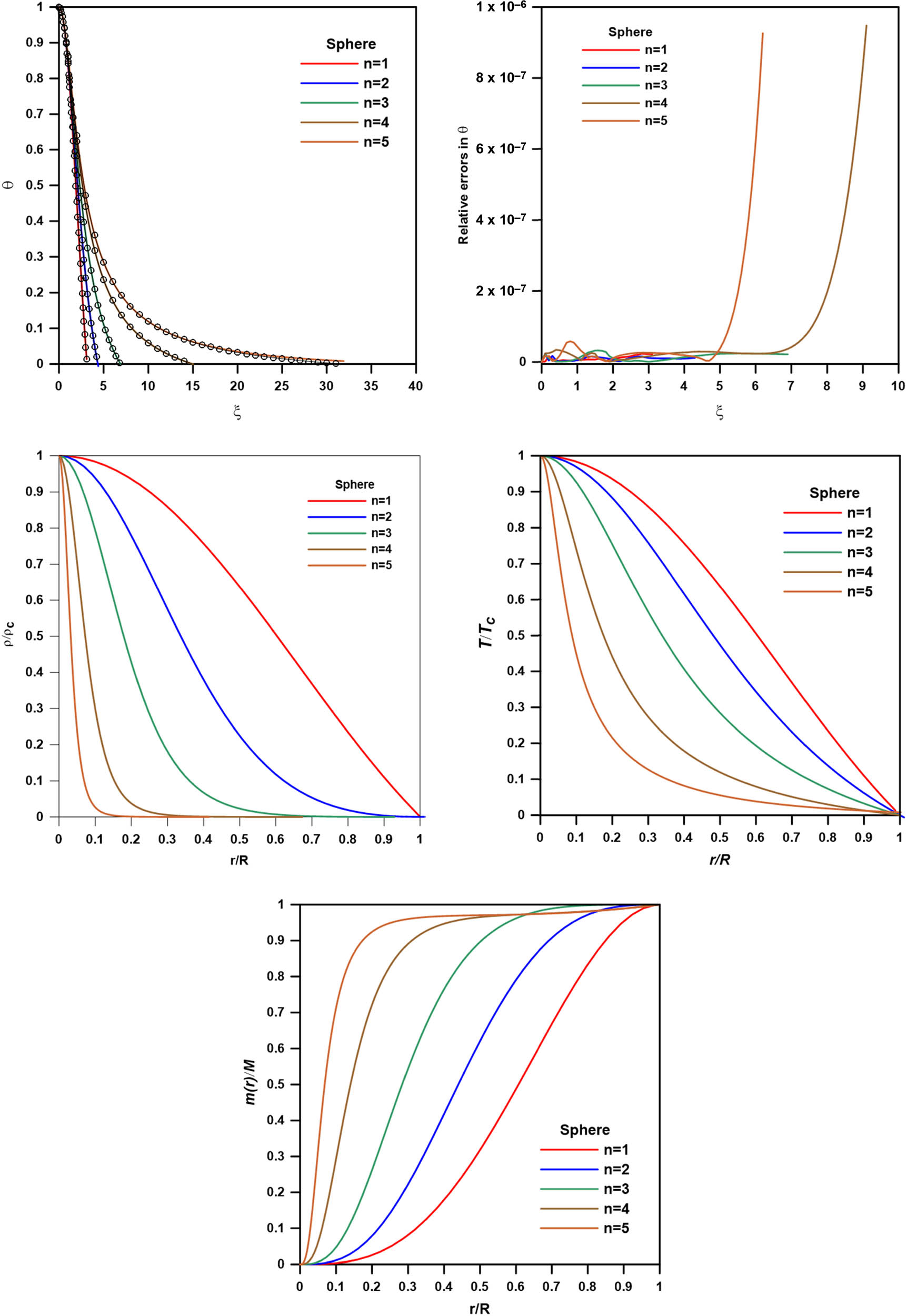
Figures 2–4 plot the accelerated Emden function for the N-dimensional polytropes calculated by ASE (solid lines) and the numerical integration (open circles). The Emden function of the polytropic sphere (the upper-left panels of Figures 2–4) converges smoothly to the zeros for n = 0–4.5; for the index of a sphere with n = 5, we truncated the calculation to ξ = 30 since it has no zeros. Also, the Emden function converges to the desired value calculated by numerical integration for the slab and cylindrical sphere. The absolute errors between the ASE and the numerical integration are also plotted for the three cases: slab, cylinder, and sphere. Comparison between ASE and numerical integration gives good agreement with maximum absolute errors of about 10⁻⁷ for polytropic gas slab, 10⁻³ for polytropic gas cylinder, and 10⁻³ for polytropic gas sphere.

$Figure 2 Emden function ( θ , upper - left panel \theta ,{\rm{upper}}\text{-}{\rm{left\; panel}} ), the absolute errors in θ \theta (upper-right panel), the density profile ( ρ / ρ c \rho \text{/}{\rho }_{\text{c}} , middle-left panel), the temperature profile ( T / T c T/{T}_{\text{c}} , middle-right panel), and the mass fraction ( m ( r ) / M m(r)/M , lower panel) calculated for the polytropic gas slab.$

Figure 2

Emden function ( θ , upper - left panel ), the absolute errors in θ (upper-right panel), the density profile ( ρ / ρ c , middle-left panel), the temperature profile ( T / T c , middle-right panel), and the mass fraction ( m ( r ) / M , lower panel) calculated for the polytropic gas slab.

$Figure 3 Emden function ( θ , upper - left panel \theta ,{\rm{upper}}\text{-}{\rm{left\; panel}} ), the absolute errors in θ \theta (upper-right panel), the density profile ( ρ / ρ c \rho /{\rho }_{\text{c}} , middle-left panel), the temperature profile ( T / T c T/{T}_{\text{c}} , middle-right panel), and the mass fraction ( m ( r ) / M m(r)/M , lower panel) calculated for polytropic gas cylinder.$

Figure 3

$Figure 4 Emden function ( θ , upper - left panel \theta ,{\rm{upper}}\text{-}{\rm{left\; panel}} ), the absolute errors in θ \theta (upper-right panel), the density profile ( ρ / ρ c \rho /{\rho }_{\text{c}} , middle-left panel), the temperature profile ( T / T c T/{T}_{\text{c}} , middle-right panel), and the mass fraction ( m ( r ) / M m(r)/M , lower panel) calculated for the polytropic gas sphere.$

Figure 4

The density fraction ( θ n = ρ / ρ c ) is depicted to show how it increases with n and approaches the polytropic slab’s central plane. The density profiles for the polytropic slab, cylinder, and sphere are shown in the upper-right panel of Figures 2–4. With increasing n and getting closer to the polytrope’s center axis, the polytropic cylinder displays the same characteristic. While the graphs of the density profiles for all polytropic slab, cylinder, and sphere models appear identical, the parameter magnitudes for the same indices decline rapidly from spherical models to cylindrical and slab models, respectively. Furthermore, in the lower-dimensional models, the magnitudes remain limited.

The relation gives the ratio of the temperature to the central temperature, which is provided by T / T c = θ n + 1 . This relation is plotted in the lower-left panels of Figures 2–4 and shows a remarkable difference for the different polytropic geometry; the change of the ratio with changing the polytropic index is small for the polytropic slab and increases for the polytropic cylinder and sphere. The fraction of mass contained within a layer has a dimensional parameter ξ to the total mass, which is given by ξ θ ′ / ξ θ ′ | ξ 1 , i.e., it is a function only the first derivative of the Emden function θ ′ . We plotted the mass fraction of the polytropes in the lower-right panel of Figures 2–4. The mass fraction increases rapidly until the points near the surface of the polytrope (r/R > 0.8) and then shows a slow increase.

We compared the current polytropic gas sphere results to several prior methods, such as Saad (2004) and Hunter (2001). Hunter (2001) employed the Euler transformation to speed the convergence of the power series. For n = 3, n = 3.5, and n = 4 spherical polytropes, respectively, 60-term, 120-term, and 300-term are required to obtain the Emden function to 7-decimal place precision out to the surface. Hunter’s Euler-transformed series converges much faster than the series in the enclosed mass proposed by Roxburgh and Stockman (1999), who reported that the series requires around 1,000 terms to converge for the polytropic indexes n = 1.5 and n = 3. Saad (2004) used a 46-term series to find the zero of the Emden function for n = 1.5 and a 24-term series for n = 3. For the slab and cylindrical polytropes, our series reached the surface of the polytrope using 20 terms and 6 × 6 Pade’ approximants. In comparison, Saad (2004) reached the surface of the polytrope with 26 and 38 terms for the slab and cylindrical, respectively.

5 Conclusion

We solved the NLE equation by constructing a recurrence relation for the coefficient a k in the power series expansion. We calculated 21 models for the polytropic slab, cylinder, and sphere. We reached the region beyond the inner points of the polytrope ( ξ ≥ 1 ) using the accelerated series (ASE, Euler–Able transformation, and Pade’ approximant). We calculated polytropic models for the slab, cylinder, and gas spheres for the range of the polytropic indices n = 0–5. The Emden function of the polytropic sphere converges smoothly to the zeros for n = 0–4.5; for the index of a sphere with n = 5, we truncated the calculation to ξ = 30 since it has no zeros. It is found that the Emden function converges to the desired value calculated by numerical integration for the slab and cylindrical sphere. Comparison between the zeros of the Emden functions for polytropes computed by ASE and the numerical one reveals good agreement with a maximum relative error of 0.1%. We conclude the results obtained in the following points:

Density profiles for the polytropic slab, cylinder, and sphere appear identical; parameter magnitudes for the same polytropic indices decrease fast from spherical to cylindrical and slab models, respectively. The central condensation ( ρ c / ρ m ) of the polytropic gas slab, cylinder, and sphere; as the polytropic index n increases, the central condensation increases rapidly. The density profile shows how it grows with n and approaches the core plane of the polytropic slab.
The polytropic cylinder exhibits the same property as the polytropic index increases and gets closer to the central axis. The density profiles for all polytropic slab, cylinder, and sphere models appear identical. Yet, the parameter magnitudes for the same indices decrease fast from spherical models to cylindrical and slab models.
The temperature to central temperature ratio ( T / T c ) varies significantly for each polytropic geometry; the change in ratio with increasing the polytropic index is minor for the polytropic slab and grows for the polytropic cylinder and sphere.
The fraction of mass contained within a layer increases rapidly until the points near the surface of the polytrope (r/R > 0.8) and then shows a slow increase.
We compared the results with numerical integration and analytical methods by different authors. This comparison shows good agreement with the solutions by Saad (2004) and is better than the results by Hunter (2001).

Acknowledgements

The authors thank the Researchers Supporting Project Number (RSPD2023R993), King Saud University, Riyadh, Saudi Arabia.

Author contributions: M.N.: conceptualization, methodology, validation, writing–original draft, visualization, and project administration; M.T.: conceptualization, software; M.A.: validation and supervision; A.I.: writing and supervision. All authors have accepted responsibility for the entire content of this manuscript and approved its submission.
Conflict of interest: The authors declare no conflict of interest.
Data availability statement: The data that support the findings of this study are available from the corresponding author upon reasonable request.

References

Abdel-Salam EA-B, Nouh MI, Elkloly EA. 2020. Analytical solution to the conformable fractional Lane-Emden type equations arising in astrophysics. Sci Afr. 8:e00386.10.1016/j.sciaf.2020.e00386Search in Google Scholar

Abd-Elhameed WM, Doha EH, Saad AS, Bassuony MA. 2016. New Galerkin operational matrices for solving Lane-Emden type equations. RMxAA. 52:83.10.1140/epjp/i2015-15052-2Search in Google Scholar

Adomian G. 1983. Stochastic systems. New York: Academic Press.Search in Google Scholar

Adomian G, Rach R, Shawagfeh NT. 1995. On the analytic solution of the Lane-Emden equation. Found Phys Lett. 8(2):161.10.1007/BF02187585Search in Google Scholar

Aitken A. 1926. XXV.—On Bernoulli's numerical solution of algebraic equations. Proc R Soc Edinburgh. 46:289.10.1017/S0370164600022070Search in Google Scholar

Bhrawy A, Alofi A. 2012. A Jacobi–Gauss collocation method for solving nonlinear Lane–Emden type equations. CNSNS. 17:62.10.1016/j.cnsns.2011.04.025Search in Google Scholar

Cao GZ, Guo L. 2011. Applied researching of ant colony optimization. Computer Knowl Technol. 7(2):437–438.Search in Google Scholar

Chandrasekhar S. 1967. Introduction to the study of stellar structure. Dover, New York: Dover Publications, Inc.Search in Google Scholar

Demodovich B, Maron I. 1973. Computational mathematics. Moscow: Mir Publishers.Search in Google Scholar

El-Essawy SH, Nouh MI, Soliman AA, Abdel Rahman HI, Abd-Elmougod GA. 2023. Monte Carlo simulation of Lane–Emden type equations arising in astrophysics, Astron Comput. 42:100665.10.1016/j.ascom.2022.100665Search in Google Scholar

El-Essawy S-H, Nouh MI, Soliman AA, Abdel Rahman H-I, Abd-Elmougod GA. 2024. A novel numerical solution to Lane-Emden type equations using Monte Carlo technique. Phys Scr. 99:015224. 10.1088/1402-4896/ad137b.Search in Google Scholar

Emden R. 1907. Gaskugeln: Anwendungen der mechanischen Wärmetheorie auf kosmologische und meteorologische Probleme. Teubner, Leipzig.Search in Google Scholar

Euler L. 1755. Institutiones Calculi Differentialis cum eius usu in Analysi Finitorum ac Doctrina Serierum. St. Petersburg: Academiae Imperialis Scientiarum.Search in Google Scholar

Ge JK, Qiu YH, Wu CM, et al. 2008. Summary of genetic algorithms research. Application Research of Computers. 25(10):291–2916.Search in Google Scholar

Horedt G-P. 1987. Topology of the Lane-Emden equation. A&A. 172:359.Search in Google Scholar

Horedt GP. 2004. Polytropes - Applications in astrophysics and related fields. Astrophysics and Space Science Library (Vol. 306). Dordrecht: Kluwer Academic Publishers.Search in Google Scholar

Hunter C. 2001. Series solutions for polytropes and the isothermal sphere. Mon Not R Astron Soc. 328:839.10.1046/j.1365-8711.2001.04914.xSearch in Google Scholar

Iqbal S, Javed A. 2011. Application of optimal homotopy asymptotic method for the analytic solution of singular Lane–Emden type equation. ApMaC. 217:7753.10.1016/j.amc.2011.02.083Search in Google Scholar

Kippenhahn R, Weigert A, Weiss A. 2012. Stellar structure and evolution. Berlin Heidelberg: Springer. 10.1007/978-3-642-30304-3.Search in Google Scholar

Lane JH. 1870. ART. IX.–On the theoretical temperature of the sun; under the hypothesis of a gaseous mass maintaining its volume by its internal heat, and depending on the laws of gases as known to terrestrial experiment. Am J Sci Arts (1820–1879). 50(148):57.10.2475/ajs.s2-50.148.57Search in Google Scholar

Maciel WJ. 2016. Introduction to stellar structure. Switzerland: Springer. 10.1007/978-3-319-16142-6.Search in Google Scholar

Milne EA. 1930. The analysis of stellar structure. Obs. 53:305.Search in Google Scholar

Morawski F, Bejger M. 2020. Neural network reconstruction of the dense matter equation of state derived from the parameters of neutron stars. A&A. 642:A78.10.1051/0004-6361/202038130Search in Google Scholar

Nouh MI. 2004. Accelerated power series solution of polytropic and isothermal gas spheres. New Astron. 9:467.10.1016/j.newast.2004.02.003Search in Google Scholar

Roxburgh IR, Stockman LM. 1999. Power series solutions of the polytrope equations. Monthly Notices of the Royal Astronomical Society. 303:46.10.1046/j.1365-8711.1999.02219.xSearch in Google Scholar

Saad AS. 2004. Symbolic analytical solution of N‐dimensional radially symmetric polytropes. Astron Nachr. 325:733. 10.1002/asna.200310255.Search in Google Scholar

Seidov Z. 2000. astro-ph/0003430.Search in Google Scholar

Shawagfeh NT. 1993. Nonperturbative approximate solution for Lane–Emden equation. J Math Phys. 34:9.10.1063/1.530005Search in Google Scholar

Wynn P. 1956. On a device for computing the em (Sn) transformation. Math Tables Aids Compt. 10:91.10.2307/2002183Search in Google Scholar

Zhang WS, Yang YH, Xu JY. 2003. Theory and application of Lattice Boltzmann method. Mod Mach. 4:4–6.Search in Google Scholar

Received: 2023-10-20

Revised: 2024-01-07

Accepted: 2024-01-24

Published Online: 2024-04-12

This work is licensed under the Creative Commons Attribution 4.0 International License.

Articles in the same Issue

https://doi.org/10.1515/astro-2022-0230

Keywords for this article

equation of state; N-dimensional polytrope; series solution; physical characteristic; stellar structure

Creative Commons

BY 4.0