Further results on permanents of Laplacian matrices of trees

Tingzeng Wu; Xiangshuai Dong

doi:10.1515/math-2025-0185

Article Open Access

Further results on permanents of Laplacian matrices of trees

Tingzeng Wu and Xiangshuai Dong

Published/Copyright: August 1, 2025

Published by

Become an author with De Gruyter Brill

Submit Manuscript Author Information Explore this Subject

$Open Mathematics$

From the journal Open Mathematics Volume 23 Issue 1

Abstract

The research on the permanents of graph matrices is one of the contemporary research topic in algebraic combinatorics. Brualdi and Goldwasser characterized the upper and lower bounds of permanents of Laplacian matrices of trees. In this article, we determined the second and third minimal permanents of the Laplacian matrices of trees, and the second maximal permanent of the Laplacian matrices of trees is given. The corresponding extremal graphs are characterized. Furthermore, we determined bounds of permanents of the Laplacian matrices of non-caterpillar trees with given graph parameters. Moreover, the corresponding extremal graphs are determined.

Keywords: tree; non-caterpillar tree; Laplacian matrix; permanent; graph parameter

MSC 2010: 05C50; 05C05; 15A15

1 Introduction

Define the permanent of a matrix M = [ m i j ] of order n with i , j ∈ { 1 , 2 , … , n } by

per M = ∑ σ ∈ Λ n ∏ i = 1 n m i σ ( i ) ,

where Λ n is a set of all permutations σ of { 1 , … , n } . Valiant [1] has shown that calculating the permanent is # P -complete even when restricted to (0, 1)-matrices.

Let G = ( V ( G ) , E ( G ) ) be a simple graph with edge set E ( G ) and vertex set V ( G ) = { v 1 , v 2 , … , v n } . For any v ∈ V ( G ) , deg ( v ) denotes the degree of vertex v in G . For convenience, deg ( v ) is simply written as d ( v ) . Let D ( G ) be the diagonal matrix whose ( i , i ) -entry is d ( v i ) , and let A ( G ) be the adjacency matrix of G . The matrix L ( G ) = D ( G ) − A ( G ) is the Laplacian matrix of G . For notation and terminology not defined, please see [2].

The permanents of adjacency matrices of graphs were first systematically studied by Merris et al. [3], and the study of analogous objects in chemical literature were started by Kasum et al. [4]. The Laplacian matrix serves as the sister matrix of the adjacency matrix, Merris et al. [3] also investigated the permanents of Laplacian matrices, and he put forward the following conjecture.

Conjecture 1.1

Let G be a graph with n vertices. Then per L ( G ) ≥ 2 ( n − 1 ) , where equality holds if and only if G is a star.

Bapat later conducted research based on this conjecture. Bapat [5] gave the proof of Conjecture 1.1. Brualdi and Goldwasser [6] highlighted two intriguing motivations for studying the Laplacian matrix. First, the Laplacian matrix of a graph holds significant importance in analyzing the number of spanning trees within the graph. Second, the Laplacian matrix offers the potential to distinguish non-isomorphic graphs in a manner that the adjacency matrix cannot achieve. Hence, Brualdi and Goldwasser started to investigate the permanents of Laplacian matrices. They characterized the lower and upper bounds for permanents of the Laplacian matrices of trees, i.e.,

Theorem 1.2

(Brualdi, [6]) If T is a tree of order n, then

2 ( n − 1 ) ≤ per L ( T ) ≤ 2 − 2 2 ( 1 + 2 ) n + 2 + 2 2 ( 1 − 2 ) n .

The left equality holds if and only if T is a star, whereas the right equality holds if and only if T is a path.

Furthermore, Brualdi and Goldwasser [6] also characterized lower bounds for permanents of the Laplacian matrices of trees with given diameter, matching or bipartition. Vrba also conducted research based on Conjecture 1.1. Vrba [7] showed the following theorem.

Theorem 1.3

(Vrba, [7]) Let G be a bipartite graph. Then

per L ( G ) ≥ 3 ∣ E ( G ) ∣ − ∣ V ( G ) ∣ + 1 ,

where equality holds if and only if G is a star.

On the basis of the studies as mentioned earlier, Li and Geng [8–12] determined the second and third minimal permanents of the Laplacian matrices of trees with given matching or bipartition, and they also characterized the first to third minimal permanents of the Laplacian matrices of trees with given domination number, maximum degree or leaves number. For more studies on permanent, see [13–20], among others.

It is interesting to continue to study the problem on the extremal values of permanents of the Laplacian matrices of trees or trees with given diameter. In this article, we focus on this problem.

This article is organized as follows. In Section 2, some basic definitions are given. In Section 3, we present some lemmas. Furthermore, we construct four graph transformations that increase or decrease the permanents of the Laplacian matrices of graphs. In Section 4, we study extremal values of permanents of the Laplacian matrices of trees, and the corresponding extremal graphs are characterized. The second minimal permanents of the Laplacian matrices of trees with given diameter is also determined. In Section 5, the extremal value of permanents of the Laplacian matrices of non-caterpillar trees are determined. Moreover, we give the minimal permanents of the Laplacian matrices of non-caterpillar trees with given bipartition or diameter. Furthermore, the corresponding extremal graphs are determined. In the final section, we conclude with a summary about permanents of the Laplacian matrices of trees.

2 Basic definitions

In this section, we will present some basic definitions.

Given a simple graph G , let G − v and G − u v denote the graphs obtained from G by deleting vertex v ∈ V ( G ) and edge u v ∈ E ( G ) , respectively. The distance d ( u , v ) is the least length of a u , v -path. The diameter of G is max u , v ∈ V ( G ) d ( u , v ) .

A tree is a connected acyclic graph, and a leaf is a vertex of degree 1. The path and star of order n are denoted by P n and S n , respectively. A double-star D S ( p , q ) is a tree obtained by joining the centre of stars S p and S q by one edge. Note that both D S ( 1 , q ) and D S ( p , 1 ) are stars. A caterpillar is a tree in which a single path (the spine) is incident to (or containing) every edge. The path is a special caterpillar. See [2]. If a tree is not a caterpillar, then the tree is called non-caterpillar tree. Suppose that T n and C n denote the set of trees with n vertices and caterpillars with n vertices, respectively. Suppose that P k + 1 = u 1 u 2 … u i … u k + 1 is a path. Assume that T n , k , i is a tree obtained from P k + 1 by attaching n − k − 1 leaves to the vertex u i . In particular, T n , k , 1 is also called the Broom graph B ( n , k ) . Assume that T n ( i − 1 , k − i + 1 , n − k − 1 ) is a tree obtain from P k + 1 by attaching a pendant path of order n − k − 1 to the vertex u i .

Let S ⊆ V ( G ) be a vertex subset. We use L S ( G ) to denote the principal submatrix of L ( G ) formed by deleting the rows and columns corresponding to all vertices of S ⊆ V ( G ) . In particular, if S = { v } , then L { v } ( G ) is simply written as L v ( G ) . Let M be an n -square matrix. The matrix M i j denotes the ( n − 1 ) -square matrix obtain from M by deleting the i th row and j th column in M .

3 Some lemmas and graph transformations

In this section, we will present some lemmas and four graph transformations, which are important to prove theorems later.

Lemma 3.1 follows from the definition of permanent and is well known.

Lemma 3.1

Let M = [ m i j ] be an n-square matrix, where i , j ∈ { 1 , 2 , … , n } . Then

per M = ∑ i m i j per M i j and per M = ∑ j m i j per M i j .

Lemma 3.2

(Wu, [21]) Let T be a tree with n ( n ≥ 3 ) vertices, and v ∈ V ( T ) . Then

d ( v ) per L v ( T ) < per L ( T ) ≤ 2 d ( v ) per L v ( T ) .

Lemma 3.3

(Brualdi, Wu, [6,22]) Let P n and B ( n , k ) be the path and Broom graph with n vertices, respectively. Let Q n be the matrix obtained from L ( P n + 1 ) by deleting the row and the column of one of the end vertices. Then

per L ( P n ) = 2 − 2 2 × ( 1 + 2 ) n + 2 + 2 2 × ( 1 − 2 ) n ,
per L ( B ( n , k ) ) = ( n − k + 1 + 2 2 ) ( 1 + 2 ) k − 1 + ( n − k + 1 − 2 2 ) ( 1 − 2 ) k − 1 ,
per L ( Q n ) = 1 2 × ( 1 + 2 ) n + 1 2 × ( 1 − 2 ) n .

Lemma 3.4

(Brualdi, [6]) Suppose that n, j, and k are positive integers with 1 ≤ k < j ≤ n + 1 2 . Then

( − 1 ) k ( per Q j − 1 per Q n − j − per Q k − 1 per Q n − k ) > 0 .

If k is even, then

per Q j − 1 per Q n − j − per Q k − 1 per Q n − k > 0 .

If k is odd, then

per Q j − 1 per Q n − j − per Q k − 1 per Q n − k < 0 .

Corollary 3.1

If n is even, then

per Q 1 per Q n − 2 < per Q 3 per Q n − 4 < … < per Q n − 2 2 per Q n 2 < per Q n − 4 2 per Q n + 2 2 < … < per Q 4 per Q n − 5 < per Q 2 per Q n − 3 .

If n is odd, then

per Q 1 per Q n − 2 < per Q 3 per Q n − 4 < … < per Q n − 1 2 per Q n − 1 2 < per Q n − 3 2 per Q n + 1 2 < … < per Q 4 per Q n − 5 < per Q 2 per Q n − 3 .

Lemma 3.5

(Wu, [22]) If v is a leaf of G, and u is the vertex adjacent to v, then

per L ( G ) = per L ( G − v ) + 2 per L u ( G − v ) .

Lemma 3.6

(Wu, [22]) Let e = u v be an edge of G, and let C G ( e ) be a set of cycles containing the edge e in G. Then

per L ( G ) = per L ( G − e ) + per L v ( G − e ) + per L u ( G − e ) + 2 per L u v ( G ) + 2 ∑ C ∈ C G ( e ) ( − 1 ) ∣ V ( C ) ∣ per L V ( C ) ( G ) .

In particular, if G is a tree, then

per L ( G ) = per L ( G − e ) + per L v ( G − e ) + per L u ( G − e ) + 2 per L u v ( G ) .

Lemma 3.7

(Brualdi, [6]) Suppose that p and q are positive integers. Then

per L ( D S ( p , q ) ) = ( 2 p − 1 ) ( 2 q − 1 ) + 1 .

Lemma 3.8

(West, [2]) A tree is a caterpillar if and only if it does not contain subtree Y as an induced subgraph, where tree Y (Figure 1).

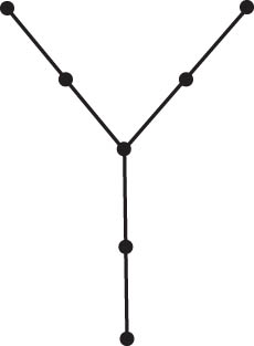
$Figure 1 Tree Y Y .$

Figure 1

Tree Y .

Lemma 3.9

(Brualdi, [6]) Let T be a tree with n vertices having diameter at least k. Then

per L ( T ) ≥ per L ( B ( n , k ) ) ,

where equality holds if and only if T is Broom graph B ( n , k ) .

Lemma 3.10

(Li, [10]) Let T n , k , i be defined as earlier. Then

per L ( T n , k , i ) = per L ( P k + 1 ) + 2 ( n − k − 1 ) per Q i − 1 per Q k − i + 1 .

Definition 3.2

Let T 1 and T 2 be two trees with ∣ V ( T 1 ) ∣ ≥ 3 and ∣ V ( T 2 ) ∣ ≥ 1 , respectively. Suppose that u , v ∈ V ( T 1 ) are a non-leaf, a leaf, respectively. Assume that w ∈ V ( T 2 ) . Denote by T the tree obtained from T 1 and T 2 by joining u and w by one edge. Denote by T [ u → v ; 1 ] the tree obtained from T by deleting the edge u w and then adding the edge v w . The resulting graph is shown in Figure 2. The transformation from T to T [ u → v ; 1 ] is named as of type I.

$Figure 2 T ⇒ T [ u → v ; 1 ] T\Rightarrow T\left[u\to v;\hspace{0.33em}1] by Transformation I.$

Figure 2

T ⇒ T [ u → v ; 1 ] by Transformation I.

Lemma 3.11

Assume that T and T [ u → v ; 1 ] are two trees defined in Definition 3.2. Then per L ( T ) ≤ per L ( T [ u → v ; 1 ] ) .

Proof

By Lemma 3.6, we obtain that

(1) per L ( T ) = per L ( T − u w ) + per L u ( T − u w ) + per L w ( T − u w ) + 2 per L u w ( T ) = [ per L ( T 1 ) + per L u ( T 1 ) ] per L ( T 2 ) + [ per L ( T 1 ) + 2 per L u ( T 1 ) ] per L w ( T 2 )

and

(2) per L ( T [ u → v ; 1 ] ) = per L ( T [ u → v ; 1 ] − v w ) + per L u ( T [ u → v ; 1 ] − v w ) + per L w ( T [ u → v ; 1 ] − v w ) + 2 per L v w ( T [ u → v ; 1 ] ) = [ per L ( T 1 ) + per L v ( T 1 ) ] per L ( T 2 ) + [ per L ( T 1 ) + 2 per L v ( T 1 ) ] per L w ( T 2 ) .

By equations (1) and (2), we obtain that

(3) per L ( T [ u → v ; 1 ] ) − per L ( T ) = [ per L v ( T 1 ) − per L u ( T 1 ) ] per L ( T 2 ) + 2 [ per L v ( T 1 ) − per L u ( T 1 ) ] per L w ( T 2 ) .

By Lemma 3.2, we obtain that d ( u ) per L u ( T 1 ) ≤ per L ( T 1 ) < 2 d ( u ) per L u ( T 1 ) and per L v ( T 1 ) ≤ per L ( T 1 ) < 2 per L v ( T 1 ) . Since d ( u ) ≥ 2 , we have per L ( T 1 ) ≥ d ( u ) per L u ( T 1 ) ≥ 2 per L u ( T 1 ) . Combining arguments as earlier, we have 2 per L u ( T 1 ) ≤ per L ( T 1 ) < 2 per L v ( T 1 ) . This implies that per L u ( T 1 ) < per L v ( T 1 ) . By equation (3) and per L u ( T 1 ) < per L v ( T 1 ) , we have per L ( T [ u → v ; 1 ] ) − per L ( T ) > 0 .□

Lemma 3.12

Let T be a tree with n vertices. Then, the tree T can be transformed into T n ( l 1 , l 2 , l 3 ) and per L ( T ) ≤ per L ( T n ( l 1 , l 2 , l 3 ) ) .

Proof

Assume that T ∉ { P n , T n ( l 1 , l 2 , l 3 ) } . Without loss of generality, we find a vertex u satisfying d ( u ) ≥ 3 and a leaf v 1 in T . By Transformation I, we move a branch joining to u from u to v 1 . We name the result graph as T ′ . If d ( u ) ≥ 3 in T ′ , we find a leaf v 2 in T . By Transformation I, we move a branch joining to u from u to v 2 . Assume that d ( u ) > 3 . Repeating this process, the degree of u will equal to 2 or 3. This implies that all vertices of degree greater than 3 in T can be changed in to the vertices of degree 2 or 3. Assume that d ( u ) = 3 . Repeating this process, the degree of u will equal to 2. This implies that all vertices of degree 3 in T can be changed into the vertices of degree 2. Thus, we conclude that the tree T can be transformed into T n ( l 1 , l 2 , l 3 ) . By Lemma 3.11, we have per L ( T ) ≤ per L ( T n ( l 1 , l 2 , l 3 ) ) .□

Definition 3.3

Let P s = u 1 , u 2 , … , u s ( s ≥ 4 ) be a path with d ( u 1 ) = 1 , d ( u s ) = 1 and d ( u i ) = 2 ( 1 < i < s ) , and let T 0 be a tree with V ( T 0 ) ≥ 2 . Denote by T the tree obtained from P s and T 0 by joining u j ( 1 < j < s ) and v by one edge. Denote by T [ u j → u 3 ; 2 ] , the tree obtained from T by deleting the edge u j v and then adding the edge u 3 v . The resulting graphs are shown in Figure 3. The transformation from T to T [ u j → u 3 ; 2 ] is named as of type II.

$Figure 3 T ⇒ T [ u j → u 3 ; 2 ] T\Rightarrow T\left[{u}_{j}\to {u}_{3};\hspace{0.33em}2] by Transformation II.$

Figure 3

T ⇒ T [ u j → u 3 ; 2 ] by Transformation II.

Lemma 3.13

Suppose that T and T [ u j → u 3 ; 2 ] are two trees defined in Definition 3.3. Then per L ( T ) ≤ per L ( T [ u j → u 3 ; 2 ] ) .

Proof

By Lemma 3.6, we obtain that

(4) per L ( T ) = per L ( T − u j v ) + per L u j ( T − u j v ) + per L v ( T − u j v ) + 2 per L u j v ( T ) = [ per L ( P s ) + per L u j ( P s ) ] per L ( T 0 ) + [ per L ( P s ) + 2 per L u j ( P s ) ] per L v ( T 0 ) = [ per L ( P s ) + per Q j − 1 per Q s − j ] per L ( T 0 ) + [ per L ( P s ) + 2 per Q j − 1 per Q s − j ] per L v ( T 0 )

and

(5) per L ( T [ u j → u 3 ; 2 ] ) = per L ( T [ u j → u 3 ; 2 ] − u 3 v ) + per L u 3 ( T [ u j → u 3 ; 2 ] − u 3 v ) + per L w ( T [ u j → u 3 ; 2 ] − u 3 v ) + 2 per L u 3 v ( T [ u j → u 3 ; 2 ] ) = [ per L ( P s ) + per L u 3 ( P s ) ] per L ( T 0 ) + [ per L ( P s ) + 2 per L u 3 ( P s ) ] per L v ( T 0 ) = [ per L ( P s ) + per Q 2 per Q s − 3 ] per L ( T 0 ) + [ per L ( P s ) + 2 per Q 2 per Q s − 3 ] per L v ( T 0 ) .

By equations (4) and (5), we obtain that

(6) per L ( T [ u j → u 3 ; 2 ] ) − per L ( T ) = ( per Q 2 per Q s − 3 − per Q j − 1 per Q s − j ) per L ( T 0 ) + 2 ( per Q 2 per Q s − 3 − per Q j − 1 per Q s − j ) per L v ( T 0 ) .

By Corollary 3.1, we have per Q 2 per Q s − 3 ≥ per Q j − 1 per Q s − j . By Equation (6), we obtain that per L ( T [ u j → u 3 ; 2 ] ) − per L ( T ) ≥ 0 .□

Definition 3.4

Let T 0 be a tree with V ( T 0 ) ≥ 2 , and let T m be a tree with m ( m ≥ 2 ) vertices. Denote by T the tree obtained from T 0 and T m by joining u ∈ V ( T 0 ) and v ∈ V ( T m ) by one edge. Denote by T [ v → u ; 3 ] the tree obtained from T 0 by attaching m leaves to u ∈ V ( T 0 ) . Suppose that these m leaves incident with u are labelled v 1 , v 2 , … , v m . The resulting graphs can be seen in Figure 4. The transformation from T to T [ v → u ; 3 ] is called type III.

$Figure 4 T ⇒ T [ v → u ; 3 ] T\Rightarrow T\left[v\to u;\hspace{0.33em}3] by Transformation III.$

Figure 4

T ⇒ T [ v → u ; 3 ] by Transformation III.

Lemma 3.14

Assume that T and T [ v → u ; 3 ] are two trees defined in Definition 3.4. Then per L ( T ) ≥ per L ( T [ v → u ; 3 ] ) .

Proof

By Lemma 3.6, we obtain that

(7) per L ( T ) = per L ( T − u v ) + per L v ( T − u v ) + per L u ( T − u v ) + 2 per L u v ( T ) = [ per L ( T m ) + per L v ( T m ) ] per L ( T 0 ) + [ per L ( T m ) + 2 per L v ( T m ) ] per L u ( T 0 ) .

By Lemma 3.5, we obtain that

(8) per L ( T [ v → u ; 3 ] ) = per L ( T [ v → u ; 3 ] − v 1 ) + 2 per L u ( T [ v → u ; 3 ] ) = per L ( T [ v → u ; 3 ] − v 1 ) + 2 per L u ( T 0 ) = per L ( T [ v → u ; 3 ] − v 1 − v 2 ) + 2 per L u ( T 0 ) + 2 per L u ( T 0 ) = per L ( T [ v → u ; 3 ] − v 1 − v 2 − v 3 ) + 2 per L u ( T 0 ) + 2 per L u ( T 0 ) + 2 per L u ( T 0 ) = … = per L ( T [ v → u ; 3 ] − v 1 − v 2 − … − v m ) + 2 m per L u ( T 0 ) = per L ( T 0 ) + 2 m per L u ( T 0 ) .

By equations (7) and (8), we know that

(9) per L ( T ) − per L ( T [ v → u ; 3 ] ) = [ per L ( T m ) + per L v ( T m ) − 1 ] per L ( T 0 ) + [ per L ( T m ) + 2 per L v ( T m ) − 2 m ] per L u ( T 0 ) .

By Theorem 1.2, we have per L ( T m ) ≥ 2 ( m − 1 ) . Since m ≥ 2 , we obtain that per L ( T m ) ≥ 2 ( m − 1 ) ≥ 2 and per L v ( T m ) ≥ 1 . This implies that per L ( T m ) + 2 per L v ( T m ) − 2 m ≥ 0 and per L ( T m ) + per L v ( T m ) − 1 > 0 . By Equation (9), we conclude that per L ( T ) − per L ( T [ v → u ; 3 ] ) > 0 .□

Definition 3.5

(Li, [10]) Let u v be a pendant edge in a bipartite graph G with n ( n ≥ 3 ) vertices, where d ( u ) = 1 . Assume that w ( ≠ v ) is a vertex of G with d ( w ) ≥ d ( v ) . Denote by G [ v → w ; 4 ] the graph obtained from T by deleting the edge u v and then adding the edge u w . The transformation from G to G [ v → w ; 4 ] is called type IV.

Lemma 3.15

(Li, [10]) Suppose that G and G [ v → w ; 4 ] be two graphs defined in Definition 3.5. Then per L ( G ) > per L ( G [ v → w ; 4 ] ) .

4 Extremal trees of permanents of the Laplacian matrices

In this section, we first give the second maximal Laplacian permanents of trees and the second and third minimal Laplacian permanent of trees.

Lemma 4.1

per L ( T n ( 2 , 2 , n − 5 ) ) = 24 + 9 2 2 ( 1 + 2 ) n − 5 + 24 − 9 2 2 ( 1 − 2 ) n − 5 .

Proof

With an appropriate ordering of the vertices of T n ( 2 , 2 , n − 5 ) , we may assume that the matrix L ( T n ( 2 , 2 , n − 5 ) ) has the following form:

L ( T n ( 2 , 2 , n − 5 ) ) = 3 − 1 0 − 1 0 − 1 0 0 … 0 0 − 1 2 − 1 0 0 … 0 0 − 1 1 − 1 2 − 1 0 0 − 1 1 0 … 0 − 1 2 − 1 0 0 0 − 1 2 − 1 … 0 0 − 1 2 ⋮ ⋮ ⋮ ⋮ ⋱ ⋮ 0 2 − 1 0 0 0 0 … − 1 1 ,

where 0 is the matrix of all 0’s.

By Lemma 3.1, expanding the permanent of matrix L ( T n ( 2 , 2 , n − 5 ) ) along row 1, we obtain that per L ( T n ( 2 , 2 , n − 5 ) ) = 3 × 3 2 × per Q n − 5 + 3 × per Q n − 5 + 3 2 × per Q n − 6 . By Lemma 3.3, we have per L ( T n ( 2 , 2 , n − 5 ) ) = 3 × 3 2 × ( 1 2 ( 1 + 2 ) n − 5 + 1 2 ( 1 − 2 ) n − 5 ) + 3 × ( 1 2 ( 1 + 2 ) n − 5 + 1 2 ( 1 − 2 ) n − 5 ) + 3 2 × ( 1 2 ( 1 + 2 ) n − 6 + 1 2 ( 1 − 2 ) n − 6 ) = 24 + 9 2 2 ( 1 + 2 ) n − 5 + 24 − 9 2 2 ( 1 − 2 ) n − 5 .□

Theorem 4.1

Suppose that T ∈ T n and T ≠ P n . Then

per L ( T ) ≤ 24 + 9 2 2 ( 1 + 2 ) n − 5 + 24 − 9 2 2 ( 1 − 2 ) n − 5 ,

where equality holds if and only if T = T n ( 2 , 2 , n − 5 ) .

Proof

By Lemma 3.12, we obtain that the tree T can be transformed into T n ( l 1 , l 2 , l 3 ) and per L ( T n ( l 1 , l 2 , l 3 ) ) > per L ( T ) . Without loss of generality, we note that l 1 ≥ l 2 ≥ l 3 . Checking the structure of T n ( l 1 , l 2 , l 3 ) , we find the longest path P l 1 + l 2 + 1 contained in T n ( l 1 , l 2 , l 3 ) . By Transformation II, the tree T n ( l 1 , l 2 , l 3 ) can be transformed into the T n ( 2 , l 3 , n − l 3 − 3 ) . By Lemma 3.11, we obtain that per L ( T n ( 2 , l 3 , n − l 3 − 3 ) ) > per L ( T n ( l 1 , l 2 , l 3 ) ) . By Transformation II, the tree T n ( 2 , l 3 , n − l 3 − 3 ) can be transformed into the T n ( 2 , 2 , n − 5 ) . By Lemma 3.11, we know that per L ( T n ( 2 , l 3 , n − l 3 − 3 ) ) ≤ per L ( T n ( 2 , 2 , n − 5 ) ) . Thus, we conclude that per ( T ) ≤ per L ( T n ( 2 , 2 , n − 5 ) ) . By Lemma 4.1, we have per L ( T ) ≤ 24 + 9 2 2 ( 1 + 2 ) n − 5 + 24 − 9 2 2 ( 1 − 2 ) n − 5 .□

Theorem 4.2

Suppose that T ∈ T n . Then each of the following holds.

If T ≠ S n , then
per L ( T ) ≥ 6 n − 14 ,
where equality holds if and only if T = D S ( 2 , n − 2 ) .
If T ≠ S n and T ≠ D S ( 2 , n − 2 ) , then
per L ( T ) ≥ 10 n − 34 ,
where equality holds if and only if T = D S ( 3 , n − 3 ) .

Proof

Assume that the diameter of T equal to l . Since T ≠ S n , we obtain that l ≥ 3 . According to the size of the diameter of T , we consider two cases as follows.

Suppose that l ≥ 4 . By Lemma 3.9, we have per L ( T ) ≥ per L ( B ( n , l ) ) . By Transformation III, Broom graph B ( n , l ) can be transformed into Broom graph B ( n , l − 1 ) . By Lemma 3.14, we obtain that per L ( B ( n , l − 1 ) ) < per L ( B ( n , l ) ) . By Lemma 3.9, we obtain that per L ( T ) ≥ per L ( B ( n , l ) ) ≥ per L ( B ( n , 4 ) ) = 14 n − 46 ( n ≥ 5 ) .

Suppose that l = 3 . It indicates that T is a double star. Define T = D S ( x , y ) , where there are x − 1 and y − 1 leaves adjoining to u and v , respectively. Without loss of generality, we note that x ≤ y . By Lemma 3.7, we have per L ( D S ( x , y ) ) = ( 2 x − 1 ) ( 2 y − 1 ) + 1 . Since x + y = n , we obtain that per L ( D S ( x , n − x ) ) = ( 2 x − 1 ) ( 2 n − 2 x − 1 ) + 1 = − 4 x 2 + 4 n x + 2 − 2 n and per L ( D S ( y , n − y ) ) = ( 2 y − 1 ) ( 2 n − 2 y − 1 ) + 1 = − 4 y 2 + 4 n y + 2 − 2 n . Define a function F ( x ) = − 4 x 2 + 4 n x + 2 − 2 n . Since x ≤ y , we have F ′ ( x ) = − 8 x + 4 n = 4 ( n − 2 x ) = 4 ( y − x ) ≥ 0 . So, F ( x ) is an increasing function on x . Since x ≥ 2 and y ≥ 2 , we conclude that F ( x ) attain minimum value when x = 2 . Direct calculating yields per L ( D S ( 2 , n − 2 ) ) = 6 n − 14 . If x = 3 , then D S ( x , y ) = D S ( 3 , n − 3 ) . By Lemma 3.7, we have per L ( D S ( 3 , n − 3 ) ) = 10 n − 34 .

Since n ≥ 5 , we have per L ( D S ( 2 , n − 2 ) ) = 6 n − 14 < 14 n − 46 = per L ( B ( n , 4 ) ) and per L ( D S ( 3 , n − 3 ) ) = 10 n − 34 < 14 n − 46 = per L ( B ( n , 4 ) ) . If T ≠ S n , then per L ( T ) ≥ per L ( D S ( 2 , n − 2 ) ) . If T ≠ S n and T ≠ D S ( 2 , n − 2 ) , it can be known that per L ( T ) ≥ per L ( D S ( 3 , n − 3 ) ) = 10 n − 34 .□

Remark

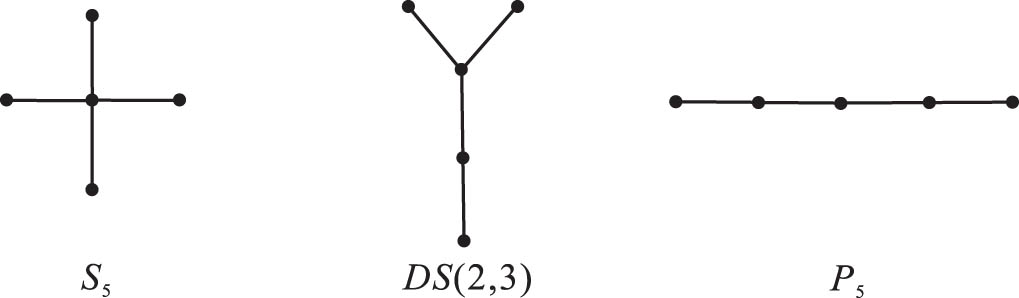
For the convenience of understanding Theorem 4.2, we enumerated all trees with five vertices (Figure 5). By simple calculation, we have per L ( S 5 ) = 8 , per L ( D S ( 2 , 3 ) ) = 16 and per L ( S 5 ) = 24 .

$Figure 5 S 5 {S}_{5} , D S ( 2,3 ) DS\left(\mathrm{2,3}) , and P 5 {P}_{5} .$

Figure 5

S 5 , D S ( 2,3 ) , and P 5 .

Next we characterize the second minimal Laplacian permanent of trees with given diameter.

Lemma 4.2

Assume that T n , k , 4 is defined as earlier. Then, per L ( T n , k , 4 ) = ( 7 n − 7 k − 2 + 7 2 2 ) ( 1 + 2 ) k − 3 + ( 7 n − 7 k − 2 − 7 2 2 ) ( 1 − 2 ) k − 3 .

Proof

By Lemma 3.10, we obtain that per L ( T n , k , 4 ) = per L ( P k + 1 ) + 2 ( n − k − 1 ) per Q 3 per Q k − 3 . By Lemma 3.3, we obtain that

□ per L ( T n , k , 4 ) = per L ( P k + 1 ) + 2 ( n − k − 1 ) per Q 3 per Q k − 3 = 2 − 2 2 ( 1 + 2 ) k + 1 + 2 + 2 2 ( 1 − 2 ) k + 1 + 2 ( n − k − 1 ) per Q 3 × ( 1 2 ( 1 + 2 ) k − 3 + 1 2 ( 1 − 2 ) k − 3 ) = ( 7 n − 7 k − 2 + 7 2 2 ) ( 1 + 2 ) k − 3 + ( 7 n − 7 k − 2 − 7 2 2 ) ( 1 − 2 ) k − 3 .

Theorem 4.3

Let T ≠ B ( n , k ) be a tree with n vertices having diameter k ≥ 7 . Then

per L ( T ) ≥ 7 n − 7 k − 2 + 7 2 2 ( 1 + 2 ) k − 3 + 7 n − 7 k − 2 − 7 2 2 ( 1 − 2 ) k − 3 ,

where equality holds if and only if T = T n , k , 4 .

Proof

There exists the longest path P k + 1 = u 1 u 2 … u i … u k + 1 in T ( ≠ B ( n , k ) ) . Repeated applications of Transformation III, T can be transformed into a caterpillar T ′ whose spine is the path P k + 1 . By Lemma 3.14, we have per L ( T ) ≥ per L ( T ′ ) . Repeated applications of Transformation IV, the caterpillar T ′ can be transformed into T n , k , a , where a ∈ { 2 , 3 , … , k } . By Lemma 3.15, we have per L ( T ′ ) ≥ per L ( T n , k , a ) . By Lemma 3.10, we have per L ( T n , k , a ) = per L ( P k + 1 ) + 2 ( n − k − 1 ) per Q a − 1 per Q k − a + 1 . Define a function

I ( a ) = per L ( P k + 1 ) + 2 ( n − k − 1 ) per Q a − 1 per Q k − a + 1 .

By Corollary 3.1, we obtain that I ( 2 ) < I ( 4 ) < I ( 6 ) < … < I ( ⌊ k + 1 2 ⌋ ) < … < I ( 7 ) < I ( 5 ) < I ( 3 ) . Since T ≠ B ( n , k ) and k ≥ 7 , we obtain that per L ( T ) ≥ per L ( T n , k , 4 ) . By Lemma 4.2, we obtain that per L ( T ) ≥ 7 n − 7 k − 2 + 7 2 2 ( 1 + 2 ) k − 3 + 7 n − 7 k − 2 − 7 2 2 ( 1 − 2 ) k − 3 .□

5 Extremal values of Laplacian permanents of non-caterpillar trees

Brualdi and Goldwasser [6] characterized extremal values of Laplacian Permanents of trees and trees with given diameter or bipartition. And all the corresponds graphs are caterpillars. Thus, it is interesting to investigate extremal values of Laplacian Permanents of non-caterpillar trees. In this section, the extremal values of Laplacian Permanents of non-caterpillar trees will be given. Moreover, we also investigate lower bound for permanents of the Laplacian matrices of non-caterpillar trees with given diameter or bipartition.

Theorem 5.1

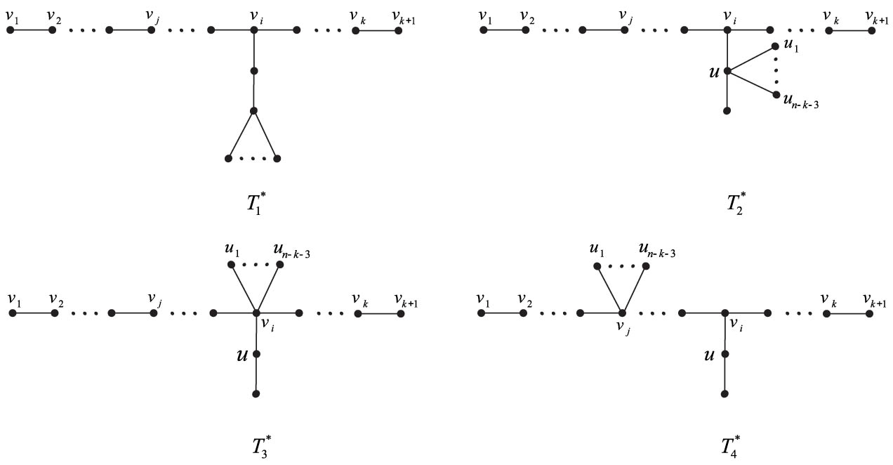
Let T ∉ C n be a tree with n vertices and n ≥ 7 . Then

per L ( T ) ≥ 54 n − 270 ,

where equality holds if and only if T = Y 3 * (Figure 6).

$Figure 6 Trees Y 1 * {Y}_{1}^{* } , Y 2 * {Y}_{2}^{* } , and Y 3 * {Y}_{3}^{* } .$

Figure 6

Trees Y 1 * , Y 2 * , and Y 3 * .

$Figure 7 Tree Y * {Y}^{* } .$

Figure 7

Tree Y * .

Proof

By Lemma 3.8, we obtain that T must contain tree Y as an induced subgraph. Repeated applications of Transformation III, each branch incident to the vertex of tree Y is changed into a star whose centre is this vertex of tree Y , and the number of leaves of the star equals to the number of vertices in that branch. The tree T can be transformed into Y * . The result graphs are shown in Figure 7. By Lemma 3.14, we have per L ( T ) ≥ per L ( Y * ) . Repeated applications of Transformation IV, we merge the leaves of subtree Y in Y * . The tree Y * can be transformed into Y 1 * , Y 2 * or Y 3 * . See Figure 6. By Lemma 3.15, we have per L ( Y * ) ≥ max { Y 1 * , Y 2 * , Y 3 * } . By Lemma 3.5, we obtain that

(10) per L ( Y 1 * ) = per L ( Y 1 * − u 1 ) + 2 per L u ( Y 1 * − u 1 ) = per L ( Y 1 * − u 1 ) + 2 per L u ( Y ) = per L ( Y 1 * − u 1 − u 2 ) + 2 per L u ( Y ) + 2 per L u ( Y ) = per L ( Y 1 * − u 1 − u 2 − u 3 ) + 2 per L u ( Y ) + 2 per L u ( Y ) + 2 per L u ( Y ) = … = per L ( Y 1 * − u 1 − u 2 − … − u n − 8 − u n − 7 ) + 2 ( n − 7 ) per L u ( Y ) = per L ( Y ) + 2 ( n − 7 ) per L u ( Y ) ,

(11) per L ( Y 2 * ) = per L ( Y 2 * − v 1 ) + 2 per L v ( Y 2 * − v 1 ) = per L ( Y 2 * − v 1 ) + 2 per L v ( Y ) = per L ( Y 2 * − v 1 − v 2 ) + 2 per L v ( Y ) + 2 per L v ( Y ) = per L ( Y 2 * − v 1 − v 2 − v 3 ) + 2 per L v ( Y ) + 2 per L v ( Y ) + 2 per L v ( Y ) = … = per L ( Y 2 * − v 1 − v 2 − … − v n − 8 − v n − 7 ) + 2 ( n − 7 ) per L v ( Y ) = per L ( Y ) + 2 ( n − 7 ) per L v ( Y )

and

(12) per L ( Y 3 * ) = per L ( Y 3 * − w 1 ) + 2 per L w ( Y 3 * − w 1 ) = per L ( Y 3 * − w 1 ) + 2 per L w ( Y ) = per L ( Y 3 * − w 1 − w 2 ) + 2 per L w ( Y ) + 2 per L w ( Y ) = per L ( Y 3 * − w 1 − w 2 − w 3 ) + 2 per L w ( Y ) + 2 per L w ( Y ) + 2 per L w ( Y ) = … = per L ( Y 3 * − w 1 − w 2 − … − w n − 8 − w n − 7 ) + 2 ( n − 7 ) per L w ( Y ) = per L ( Y ) + 2 ( n − 7 ) per L w ( Y ) .

With an appropriate ordering of the vertices of tree Y , we may assume that the matrices L u ( Y ) , L v ( Y ) , and L w ( Y ) have the following forms:

(13) L u ( Y ) = 3 − 1 0 − 1 0 0 − 1 2 − 1 0 0 0 0 − 1 1 0 0 0 − 1 0 0 2 − 1 0 0 0 0 − 1 1 0 0 0 0 0 0 1 ,

(14) L v ( Y ) = 3 − 1 0 − 1 0 − 1 − 1 2 − 1 0 0 0 0 − 1 1 0 0 0 − 1 0 0 2 − 1 0 0 0 0 − 1 1 0 − 1 0 0 0 0 2

and

(15) L w ( Y ) = 2 − 1 0 0 0 0 − 1 1 0 0 0 0 0 0 2 − 1 0 0 0 0 − 1 1 0 0 0 0 0 0 2 − 1 0 0 0 0 − 1 1 .

Direct calculating yields that per L u ( Y ) = 33 , per L v ( Y ) = 75 and per L w ( Y ) = 27 . Hence, per L v ( Y ) > per L u ( Y ) > per L w ( Y ) = 27 . By equations (10), (11), and (12), we have per L ( Y 2 * ) > per L ( Y 1 * ) > per L ( Y 3 * ) . By direct calculating, we obtain that per L ( Y ) = 108 . Hence, it can be known that per L ( Y 3 * ) = per L ( Y ) + 2 ( n − 7 ) per L w ( Y ) = 54 n − 270 . Base on arguments as earlier, we obtain that per L ( T ) ≥ 54 n − 270 , where equality holds if and only if T = Y 3 * .□

By Theorem 4.1, we obtain the following Theorem 5.2 immediately.

Theorem 5.2

Let T ∉ C n be a tree with n ≥ 7 vertices. Then

per L ( T ) ≤ 24 + 9 2 2 ( 1 + 2 ) n − 5 + 24 − 9 2 2 ( 1 − 2 ) n − 5 ,

where equality holds if and only if T = T n ( 2 , 2 , n − 5 ) .

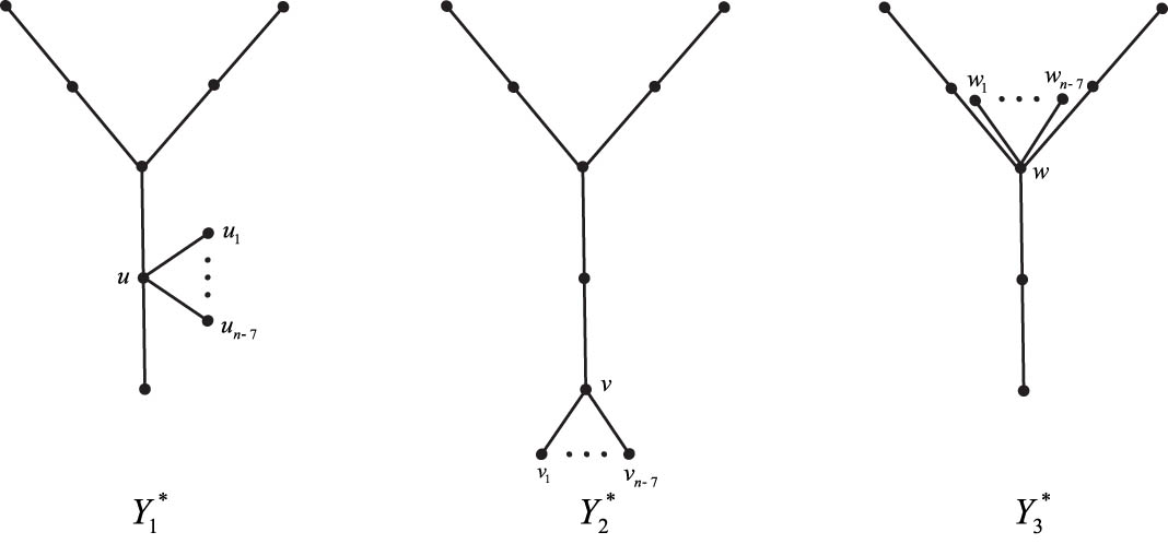
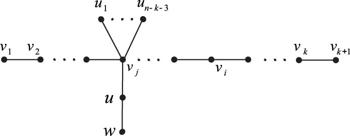
Theorem 5.3

Let T ∉ C n be a tree with n ≥ 7 vertices having diameter k. Then

per L ( T ) ≥ ( 21 n − 21 k − 34 + 21 2 2 ) ( 1 + 2 ) k − 3 + ( 21 n − 21 k − 34 − 21 2 2 ) ( 1 − 2 ) k − 3 ,

where equality holds if and only if T = T * (Figure 8).

$Figure 8 Tree T * {T}^{* } .$

Figure 8

Tree T * .

$Figure 9 Tree T k + 3 ( 2 , i − 1 , k − i + 1 ) {T}_{k+3}\left(2,i-1,k-i+1) .$

Figure 9

Tree T k + 3 ( 2 , i − 1 , k − i + 1 ) .

$Figure 10 Trees T 1 * {T}_{1}^{* } , T 2 * {T}_{2}^{* } , T 3 * {T}_{3}^{* } , and T 4 * {T}_{4}^{* } .$

Figure 10

Trees T 1 * , T 2 * , T 3 * , and T 4 * .

Proof

There exists the longest path P k + 1 = v 1 v 2 … v i … v k + 1 in T . Since T ∉ C n and the definition of caterpillar, we conclude that T must contain the following tree T k + 3 ( 2 , i − 1 , k − i + 1 ) as an induced subgraph, where 3 ≤ i ≤ k − 1 . The structure of tree T k + 3 ( 2 , i − 1 , k − i + 1 ) (Figure 9). Repeated applications of Transformation III, each branch incident to the vertex of tree T k + 3 ( 2 , i − 1 , k − i + 1 ) is changed into a star whose centre is this vertex of tree T k + 3 ( 2 , i − 1 , k − i + 1 ) , and the number of leaves of the star equals to the number of vertices in that branch. The tree T can be transformed into T ¯ . By Lemma 3.14, we have per L ( T ) ≥ per L ( T ¯ ) . Repeated applications of Transformation IV, we merge the leaves of subtree T k + 3 ( 2 , i − 1 , k − i + 1 ) in T . The tree T ¯ can be transformed into T 1 * , T 2 * , T 3 * , or T 4 * (Figure 10). By Lemma 3.15, we have per L ( T ¯ ) ≥ max { T 1 * , T 2 * , T 3 * , T 4 * } . By Lemma 3.14, we have per L ( T 1 * ) > per L ( T 2 * ) . By Lemma 3.6, we obtain that

(16) per L ( T k + 3 ( 2 , i − 1 , k − i + 1 ) ) = per L ( T k + 3 ( 2 , i − 1 , k − i + 1 ) − u v i ) + per L v i ( T k + 3 ( 2 , i − 1 , k − i + 1 ) − u v i ) + per L u ( T k + 3 ( 2 , i − 1 , k − i + 1 ) − u v i ) + per L u v i ( T k + 3 ( 2 , i − 1 , k − i + 1 ) − u v i ) = 3 per L ( P k + 1 ) + 4 per L v i ( P k + 1 )

and

(17) per L ( T 2 * ) = per L ( T 2 * − u v i ) + per L v i ( T 2 * − u v i ) + per L u ( T 2 * − u v i ) + per L u v i ( T 2 * − u v i ) = ( 2 ( n − k − 3 + 1 ) + 1 ) per L ( P k + 1 ) + ( 2 ( n − k − 3 + 1 ) + 2 ) per L v i ( P k + 1 ) = ( 2 n − 2 k − 3 ) per L ( P k + 1 ) + ( 2 n − 2 k − 2 ) per L v i ( P k + 1 ) .

By Lemma 3.5, we obtain that

(18) per L ( T 3 * ) = per L ( T 3 * − u 1 ) + 2 per L v i ( T 3 * − u 1 ) = per L ( T 3 * − u 1 ) + 2 per L v i ( T k + 3 ( 2 , i − 1 , k − i + 1 ) ) = per L ( T 3 * − u 1 − u 2 ) + 2 per L v i ( Y ) + 2 per L v i ( T k + 3 ( 2 , i − 1 , k − i + 1 ) ) = per L ( T 3 * − u 1 − u 2 − u 3 ) + 2 per L v i ( T k + 3 ( 2 , i − 1 , k − i + 1 ) ) + 2 per L v i ( T k + 3 ( 2 , i − 1 , k − i + 1 ) ) + 2 per L v i ( T k + 3 ( 2 , i − 1 , k − i + 1 ) ) = … = per L ( T 3 * − u 1 − u 2 − … − u n − k − 4 − u n − k − 3 ) + 2 ( n − k − 3 ) per L v i ( T k + 3 ( 2 , i − 1 , k − i + 1 ) ) = per L ( T k + 3 ( 2 , i − 1 , k − i + 1 ) ) + 2 ( n − k − 3 ) per L v i ( T k + 3 ( 2 , i − 1 , k − i + 1 ) ) .

By observing structures of L v i ( T k + 3 ( 2 , i − 1 , k − i + 1 ) ) and L v i ( P k + 1 ) , we obtain that

(19) per L v i ( T k + 3 ( 2 , i − 1 , k − i + 1 ) ) = 3 per L v i ( P k + 1 ) .

By substituting (16) and (19) into (18), we have

(20) per L ( T 3 * ) = 3 per L ( P k + 1 ) + ( 6 n − 6 k − 14 ) per L v i ( P k + 1 ) .

By (17) and (20), we obtain that

per L ( T 2 * ) − per L ( T 3 * ) = 2 ( n − k − 3 ) per L ( P k + 1 ) − 4 ( n − k − 3 ) per L v i ( P k + 1 ) .

By Lemma 3.1, we have per L ( P k + 1 ) > d ( v i ) per L v i ( P k + 1 ) . Since d ( v i ) ≥ 2 , we obtain that per L ( P k + 1 ) > d ( v i ) per L v i ( P k + 1 ) ≥ 2 per L v i ( P k + 1 ) . Hence, per L ( T 2 * ) − per L ( T 3 * ) = 2 ( n − k − 3 ) per L ( P k + 1 ) − 4 ( n − k − 3 ) per L v i ( P k + 1 ) = 2 ( n − k − 3 ) ( per L ( P k + 1 ) − 2 per L v i ( P k + 1 ) ) > 0 . Set n − k − 3 = 1 . By Lemma 3.15, we have per L ( T 4 * ) > per L ( T 3 * ) . Set n − k − 3 ≥ 2 . We may transform T 4 * into T 5 * (Figure 11). By the definition of T n , k , i , we have T 5 * − w − u = T n − 2 , k , j . By Lemma 3.6, we obtain that

(21) per L ( T 4 * ) = per L ( T 4 * − u v i ) + per L v i ( T 4 * − u v i ) + per L u ( T 4 * − u v i ) + per L u v i ( T 4 * − u v i ) = 3 per L ( T n − 2 , k , j ) + 4 per L v i ( T n − 2 , k , j )

and

(22) per L ( T 5 * ) = per L ( T 5 * − u v j ) + per L v j ( T 5 * − u v j ) + per L u ( T 5 * − u v j ) + per L u v j ( T 5 * − u v j ) = 3 per L ( T n − 2 , k , j ) + 4 per L v j ( T n − 2 , k , j ) .

By Lemma 3.1, we have

2 d T n − 2 , k , j ( v i ) per L v i ( T n − 2 , k , j ) > per L ( T n − 2 , k , j ) > d T n − 2 , k , j ( v i ) per L v i ( T n − 2 , k , j ) .

Since d T n − 2 , k , j ( v i ) = 2 , we have

per L v i ( T n − 2 , k , j ) > 1 2 d T n − 2 , k , j ( v i ) per L ( T n − 2 , k , j ) = 1 4 per L ( T n − 2 , k , j ) .

So, we conclude that per L ( T 4 * ) = 3 per L ( T n − 2 , k , j ) + 4 per L v i ( T n − 2 , k , j ) > 3 per L ( T n − 2 , k , j ) + per L ( T n − 2 , k , j ) . Since n − k − 3 ≥ 2 , we have d T n − 2 , k , j ( v j ) ≥ 4 . By Lemma 3.2, we obtain that per L ( T n − 2 , k , j ) > d T n − 2 , k , j ( v j ) per L v j ( T n − 2 , k , j ) . Thus, we conclude that per L v j ( T n − 2 , k , j ) < 1 d T n − 2 , k , j ( v j ) × per L ( T n − 2 , k , j ) < 1 4 per L ( T n − 2 , k , j ) . This indicates that per L ( T 5 * ) = 3 per L ( T n − 2 , k , j ) + 4 per L v j ( T n − 2 , k , j ) < 3 per L ( T n − 2 , k , j ) + per L ( T n − 2 , k , j ) . It is easy to obtain that per L ( T 4 * ) > per L ( T 5 * ) .

Combining arguments mentioned earlier, we have per L ( T ) > per L ( T 3 * ) or per L ( T ) > per L ( T 5 * ) . Without loss of generality, we consider per L ( T 3 * ) . By Lemma 3.5, we obtain that

(23) per L ( T 3 * ) = per L ( T 3 * − u 1 ) + 2 per L v i ( T 3 * − u 1 ) = per L ( T 3 * − u 1 ) + 2 per L v i ( T k + 3 ( 2 , i − 1 , k − i + 1 ) ) = per L ( T 3 * − u 1 − u 2 ) + 2 per L v i ( T k + 3 ( 2 , i − 1 , k − i + 1 ) ) + 2 per L v i ( T k + 3 ( 2 , i − 1 , k − i + 1 ) ) = per L ( T 3 * − u 1 − u 2 − u 3 ) + 2 per L v i ( T k + 3 ( 2 , i − 1 , k − i + 1 ) ) + 2 per L v i ( T k + 3 ( 2 , i − 1 , k − i + 1 ) ) + 2 per L v i ( T k + 3 ( 2 , i − 1 , k − i + 1 ) ) = … = per L ( T 3 * − u 1 − u 2 − … − u n − k − 4 − u n − k − 3 ) + 2 ( n − k − 3 ) per L v i ( T k + 3 ( 2 , i − 1 , k − i + 1 ) ) = per L ( T k + 3 ( 2 , i − 1 , k − i + 1 ) ) + 2 ( n − k − 3 ) per L v i ( T k + 3 ( 2 , i − 1 , k − i + 1 ) ) .

By substituting (16) and (19) into (23), we have per L ( T 3 * ) = 3 per L ( P k ) + ( 6 n − 6 k − 14 ) per L v i ( P k ) . Define a function H ( i ) = per L ( T 3 * ) = 3 per L ( P k ) + ( 6 n − 6 k − 14 ) per L v i ( P k ) . By Corollary 3.1, we have H ( 2 ) < H ( 4 ) < H ( 6 ) < … < H ( ⌊ k + 1 2 ⌋ ) < … < H ( 7 ) < H ( 5 ) < H ( 3 ) . Since T ∉ C n , it is easy to see that H ( i ) attains the maximum value if and only if i = 4 . Moreover, the corresponding extremal graph is T * . See Figure 8. So, we conclude that per L ( T 3 * ) ≥ per L ( T * ) and per L ( T 5 * ) ≥ per L ( T * ) . It indicates that per L ( T ) ≥ per L ( T * ) .

This completes the proof of the theorem.□

$Figure 11 Tree T 5 * {T}_{5}^{* } .$

Figure 11

Tree T 5 * .

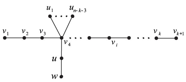
Theorem 5.4

Let T is a tree with n ( n ≥ 8 ) vertices having a ( p , q ) -bipartition with 4 ≤ p ≤ q . If T ∉ C n , then

per L ( T ) ≥ ( 6 p − 15 ) ( 6 q − 7 ) + 9 ,

where equality holds if and only if T = Y 6 * (Figure 12).

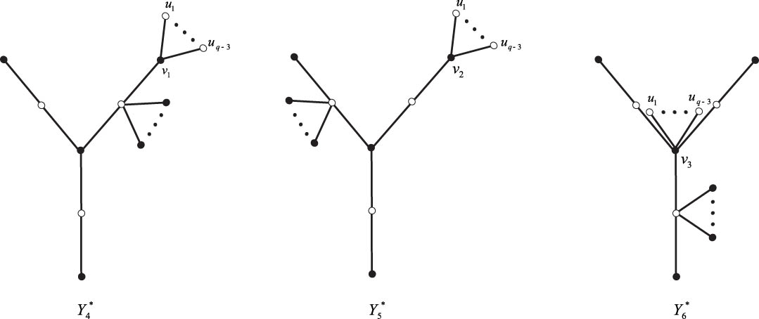
$Figure 12 Trees Y 4 * {Y}_{4}^{* } , Y 5 * {Y}_{5}^{* } , and Y 6 * {Y}_{6}^{* } .$

Figure 12

Trees Y 4 * , Y 5 * , and Y 6 * .

Proof

According to the structure of tree T , we consider two cases, i.e., T = Y * and T ≠ Y * . See Figure 12. We shall label the vertices of Y * . The vertices in the same bipartition are labelled the same colour.

Case 1 Assume that T = Y * . Assume that the number of vertices labelled white equals p , and the number of vertices labelled black equals q . Repeated applications of Transformation IV, we merge the leaves of tree Y * which belong to the same bipartition. The tree T can be transformed into Y 4 * , Y 5 * or Y 6 * . See Figure 12. By Lemma 3.15, we have per L ( T ) ≥ max { Y 4 * , Y 5 * , Y 6 * } . For convenience, we note that Y ′ = Y 4 * − u 1 − u 2 − … − u q − 4 − u q − 3 .

By Lemma 3.5, we obtain that

(24) per L ( Y 4 * ) = per L ( Y 4 * − u 1 ) + 2 per L v 1 ( Y 4 * − u 1 ) = per L ( Y 4 * − u 1 ) + 2 per L v 1 ( Y ′ ) = per L ( Y 4 * − u 1 − u 2 ) + 2 per L v 1 ( Y ′ ) + 2 per L v 1 ( Y ′ ) = per L ( Y 4 * − u 1 − u 2 − u 3 ) + 2 per L v 1 ( Y ′ ) + 2 per L v 1 ( Y ′ ) + 2 per L v 1 ( Y ′ ) = … = per L ( Y 4 * − u 1 − u 2 − … − u q − 4 − u q − 3 ) + 2 ( q − 3 ) per L v 1 ( Y ′ ) = per L ( Y ′ ) + 2 ( q − 3 ) per L v 1 ( Y ′ ) ,

(25) per L ( Y 5 * ) = per L ( Y 5 * − u 1 ) + 2 per L v 2 ( Y 5 * − u 1 ) = per L ( Y 5 * − u 1 ) + 2 per L v 2 ( Y ′ ) = per L ( Y 5 * − u 1 − u 2 ) + 2 per L v 2 ( Y ′ ) + 2 per L v 2 ( Y ′ ) = per L ( Y 5 * − u 1 − u 2 − u 3 ) + 2 per L v 2 ( Y ′ ) + 2 per L v 2 ( Y ′ ) + 2 per L v 2 ( Y ′ ) = … = per L ( Y 5 * − u 1 − u 2 − … − u q − 4 − u q − 3 ) + 2 ( q − 3 ) per L v 2 ( Y ′ ) = per L ( Y ′ ) + 2 ( q − 3 ) per L v 2 ( Y ′ )

and

(26) per L ( Y 6 * ) = per L ( Y 6 * − u 1 ) + 2 per L v 3 ( Y 6 * − u 1 ) = per L ( Y 6 * − u 1 ) + 2 per L v 3 ( Y ′ ) = per L ( Y 6 * − u 1 − u 2 ) + 2 per L v 3 ( Y ′ ) + 2 per L v 3 ( Y ′ ) = per L ( Y 6 * − u 1 − u 2 − u 3 ) + 2 per L v 3 ( Y ′ ) + 2 per L v 3 ( Y ′ ) + 2 per L v 3 ( Y ′ ) = … = per L ( Y 6 * − u 1 − u 2 − … − u q − 4 − u q − 3 ) + 2 ( q − 3 ) per L v 3 ( Y ′ ) = per L ( Y ′ ) + 2 ( q − 3 ) per L v 3 ( Y ′ ) .

With an appropriate ordering of the vertices of Y ′ , we may assume that the matrices L v 1 ( Y ′ ) , L v 2 ( Y ′ ) , and L v 3 ( Y ′ ) have the following form:

(27) L v 1 ( Y ′ ) = 3 − 1 0 − 1 0 − 1 − 1 2 − 1 0 − 1 1 0 − 1 2 − 1 0 − 1 1 − 1 p − 2 − 1 − 1 … − 1 − 1 1 − 1 1 0 ⋮ ⋱ − 1 1 ,

(28) L v 2 ( Y ′ ) = 3 − 1 0 − 1 − 1 − 1 2 − 1 0 − 1 1 0 − 1 2 − 1 p − 2 − 1 − 1 … − 1 − 1 1 − 1 1 0 ⋮ ⋱ − 1 1 ,

and

(29) L v 3 ( Y ′ ) = 2 − 1 − 1 1 2 − 1 0 − 1 1 p − 2 − 1 − 1 … − 1 − 1 1 − 1 1 0 ⋮ ⋱ − 1 1 ,

where 0 is the matrix of all 0’s.

Direct computations yield per L v 1 ( Y ′ ) = 66 ( p − 4 ) + 75 , per L v 2 ( Y ′ ) = 44 ( p − 4 ) + 66 , and per L v 3 ( Y ′ ) = 18 ( p − 4 ) + 27 . By equations (24), (25), (26), and per L v 1 ( Y ) > per L v 2 ( Y ) > per L v 3 ( Y ) = 27 , we have per L ( Y 4 * ) > per L ( Y 5 * ) > per L ( Y 6 * ) . Since the structure of Y ′ is the same as the structure of Y 1 * in Theorem 5.1, we have per L ( Y ′ ) = 108 + 2 ( p − 4 ) × 33 = 108 + 66 ( p − 4 ) . By equations (24) and per L v 1 ( Y ′ ) = 66 ( p − 4 ) + 75 , we obtain that per L ( Y 6 * ) = 108 + 66 ( p − 4 ) + 2 ( q − 3 ) ( 66 ( p − 4 ) + 75 ) = ( 6 p − 15 ) ( 6 q − 7 ) + 9 . Assume that the number of vertices labelled white equals q , and the number of vertices labelled black equals p . Similarly, we obtain that per L ( Y 4 * ) > per L ( Y 5 * ) > per L ( Y 6 * ) . Direct calculating yields per L ( Y 6 * ) = 108 + 66 ( q − 4 ) + 2 ( p − 3 ) ( 66 ( q − 4 ) + 75 ) = ( 6 q − 15 ) ( 6 p − 7 ) + 9 . Since ( 6 q − 15 ) ( 6 p − 7 ) + 9 − [ ( 6 p − 15 ) ( 6 q − 7 ) + 9 ] = 38 ( q − p ) ≥ 0 , we have per T ≥ ( 6 p − 15 ) ( 6 q − 7 ) + 9 . And equality holds if and only if T = Y 6 * .

Case 2 Assume that T ≠ Y * . This implies that p ≥ 4 and q ≥ 4 . There exist a leaf g not adjacent to the vertices of Y . Let g h be a pendant edge. Denote by V 1 and V 2 be the bipartition of the vertices of T with ∣ V 1 ∣ = p and ∣ V 2 ∣ = q . If g ∈ V 1 , then the vertices of T are labelled g , h , g 2 , … , g p , h 2 , … , h q , where V 1 = { g , g 2 , … , g p } and V 2 = { h , h 2 , … , h q } . If g ∈ V 2 , then the vertices of T are labelled g , h , g 2 , … , g q , h 2 , … , h p , where V 2 = { g , g 2 , … , g q } and V 2 = { h , h 2 , … , h p } .

Suppose that T − g = Y * . This means that d u = 2 . Without loss of generality, we assume that g ∈ V 1 . We find a non-leaf h i of V 2 in tree T − g . By Transformation IV, T can be changed into T [ h → h i ; 4 ] , where T [ h → h i ; 4 ] = T − g h + g h i . By Lemma 3.15, we have per ( T ) > per ( T [ h → h i ; 4 ] ) . Since T − g = Y * , we obtain that per ( T [ h → h i ; 4 ] ) = Y * . By Case 1, Theorem 5.4 holds.

Suppose that T − g ≠ Y * . We will show the theorem by induction on n . Cvetković et al. [23] enumerated all tree with n ( 8 ≤ n ≤ 10 ) vertices. By employing Maple 18.0, we calculate the Laplacian permanents of all trees with n ( 8 ≤ n ≤ 10 ) vertices, and conclude Theorem 5.4 are true. Assume that Theorem 5.4 holds for n = m ( m > 10 ) . We shall prove that Theorem 5.4 holds for n = m + 1 = p + q . By Lemma 3.5, we obtain that

(30) per L ( T ) = per L ( T − g ) + 2 per L h ( T − g ) .

Set g ∈ V 1 . It means that ∣ V ( Y ) ∩ V 1 ∣ = 4 . Without loss of generality, we note that the vertices of Y in Y * are g 2 , g 3 , g 4 , g 5 , h 2 , h 3 , and h 4 , where g 2 is the centre of Y . Tree T − g has a ( p − 1 , q ) -bipartition. By induction hypothesis, we have

(31) per L ( T − g ) ≥ ( 6 p − 21 ) ( 6 q − 7 ) + 9 .

With an appropriate ordering of the vertices of T − g , we may assume that the matrix L h ( T − g ) has the following form:

(32) L h ( T − g ) = d ( g 2 ) ⋱ C d ( g p ) d ( h 2 ) C ⊤ ⋱ d ( h q ) ,

where the matrix C ⊤ is the transpose of the matrix C . Since T has p + q − 1 edges, we obtain that the number of − 1 ’s in C is p + q − 1 − d ( h ) . Since all diagonal entries of the matrix (32) are positive, we have

(33) per L h ( T − g ) ≥ d ( g 2 ) … d ( g p ) d ( h 2 ) … d ( h q ) + p + q − 1 − d ( h ) .

According to the bipartition of Y , we consider two cases. Since d ( h 2 ) + … + d ( h q ) = p + q − 1 − d ( h ) , d ( h 2 ) ≥ 2 , d ( h 3 ) ≥ 2 , and d ( h 4 ) ≥ 2 , we obtain that

(34) d ( h 2 ) … d ( h q ) ≥ 2 × 2 × 2 × 1 … 1 ( ( p + q − 1 − d h ) − ( q − 2 − 3 ) − 2 − 2 − 2 ) = 8 ( p − d ( h ) − 2 ) .

Since d ( g 2 ) + … + d ( g p ) = p + q − 1 − 1 and d ( g 2 ) ≥ 3 , we conclude that

(35) d ( g 2 ) … d ( g p ) ≥ 3 × 1 … 1 ( ( p + q − 2 ) − ( p − 2 − 1 ) − 3 ) = 3 ( q − 2 ) .

Since ∣ V ( Y ) ∩ V 1 ∣ = 4 , we have d ( h ) ≤ p − 3 . So, by equations (33), (34), and (35), we obtain that

per L h ( T − g ) ≥ 3 ( q − 2 ) × 8 ( p − d ( h ) − 2 ) + p + q − d ( h ) − 1 ≥ 3 ( q − 2 ) × 8 × 1 + q − 1 = 25 q − 49 .

By Equations q ≥ 4 , (31) and (30), we have

per L ( T ) ≥ ( 6 p − 21 ) ( 6 q − 7 ) + 2 ( 25 q − 49 ) = ( 6 p − 15 ) ( 6 q − 7 ) + 9 + ( 32 q − 77 ) > ( 6 p − 15 ) ( 6 q − 7 ) + 9 .

Set g ∈ V 2 . This implies that ∣ V ( Y ) ∩ V 2 ∣ = 3 and ∣ V ( Y ) ∩ V 1 ∣ = 3 . Without loss of generality, we note that the vertices of Y in Y * are g 2 , g 3 , g 4 , h 2 , h 3 , h 4 , and h 5 , where h 2 is the centre of Y . Tree T − g has a ( p , q − 1 ) -bipartition. By induction hypothesis, we have

(36) per L ( T − g ) ≥ ( 6 p − 15 ) ( 6 q − 13 ) + 9 .

With an appropriate ordering of the vertices of T − g , we may assume that the matrix L h ( T − g ) has the following form:

L h ( T − g ) = d ( g 2 ) ⋱ C d ( g q ) d ( h 2 ) C ⊤ ⋱ d ( h p ) ,

where the matrix C ⊤ is the transpose of the matrix C . Since d ( h 2 ) + … + d ( h p ) = p + q − 1 − d ( h ) and d ( h 2 ) ≥ 3 , we obtain that

(37) d ( h 2 ) … d ( h p ) ≥ 3 × 1 … 1 ( ( p + q − 1 − d ( h ) ) − ( p − 2 − 1 ) − 3 ) = 3 ( q − d ( h ) − 1 ) .

Since d ( g 2 ) + … + d ( g q ) = p + q − 1 − 1 , d ( g 2 ) ≥ 2 , d ( g 3 ) ≥ 2 and d ( g 4 ) ≥ 2 , we have

(38) d ( g 2 ) … d ( g q ) ≥ 2 × 2 × 2 × 1 … 1 ( ( p + q − 2 ) − ( q − 2 − 3 ) − 2 − 2 − 2 ) = 8 ( p − 3 ) .

Since ∣ V ( Y ) ∩ V 1 ∣ = 3 , we have d ( h ) ≤ q − 2 . Hence, by equations (33), (37), and (38), we have

per L h ( T − g ) ≥ 8 ( p − 3 ) × 3 ( q − d ( h ) − 1 ) + p + q − d ( h ) − 1 ≥ 8 ( q − 3 ) × 3 × 1 + p − 1 = 25 p − 73 .

By p ≥ 4 , (31) and (30), we have

per L ( T ) ≥ ( 6 p − 15 ) ( 6 q − 13 ) + 9 + 2 ( 25 p − 73 ) = ( 6 p − 15 ) ( 6 q − 7 ) + 9 + ( 32 p − 101 ) > ( 6 p − 15 ) ( 6 q − 7 ) + 9 .

Combining Case 1 and Case 2, Theorem 5.4 holds.□

6 Summary

In this article, we determined the extremal permanents of Laplacian matrices of trees and non-caterpillar trees. And the corresponding extremal graphs are also determined. In general, it is difficult to evaluate permanents of Laplacian matrices of graphs. The permanents of Laplacian matrices of general graphs or special graphs (such as unicyclic graphs and bipartite graphs) are worthy of study.

Acknowledgments

The authors are grateful for the reviewer’s valuable comments that improved the manuscript.

Funding information: This research was supported by NSFC (No. 12261071) and NSF of Qinghai Province (No. 2025-ZJ-902T).
Author contributions: All authors have accepted responsibility for the entire content of this manuscript and consented to its submission to the journal, reviewed all the results, and approved the final version of the manuscript. XD provided all figures. TW prepared the manuscript with contributions from the co-author.
Conflict of interest: The authors state no conflict of interest.
Data availability statement: No data were used to support this study.

References

[1] L. G. Valiant, The complexity of computing the permanent, Theoret. Comput. Sci. 8 (1979), no. 2, 189–201, DOI: https://doi.org/10.1016/0304-3975(79)90044-6. 10.1016/0304-3975(79)90044-6Search in Google Scholar

[2] D. B. West, Introduction to Graph Theory, Prentice Hall, Upper Saddle River, NJ, 1996. Search in Google Scholar

[3] R. Merris, K. R. Rebman, and W. Watkins, Permanental polynomials of graphs, Linear Algebra Appl. 38 (1981), 273–288, DOI: https://doi.org/10.1016/0024-3795(81)90026-4. 10.1016/0024-3795(81)90026-4Search in Google Scholar

[4] D. Kasum, N. Trinajstić, and I. Gutman, Chemical graph theory. III. On permanental polynomial, Croat. Chem. Acta 54 (1981), 321–328. Search in Google Scholar

[5] R. B. Bapat, A bound for the permanent of the Laplacian matrix, Linear Algebra Appl. 74 (1986), 219–223, DOI: https://doi.org/10.1016/0024-3795(86)90124-2. 10.1016/0024-3795(86)90124-2Search in Google Scholar

[6] R. A. Brualdi and J. L. Goldwasser, Permanent of the Laplacian matrix of trees and bipartite graphs, Discrete Math. 48 (1984), no. 1, 1–21, DOI: https://doi.org/10.1016/0012-365X(84)90127-4. 10.1016/0012-365X(84)90127-4Search in Google Scholar

[7] A. Vrba, The permanent of the Laplacian matrix of a bipartite graph, Czechoslovak Math. J. 36 (1986), no. 1, 7–17, DOI: https://doi.org/10.21136/cmj.1986.102059. 10.21136/CMJ.1986.102059Search in Google Scholar

[8] S. Li and L. Zhang, Permanental bounds for the signless Laplacian matrix of a unicyclic graph with diameter d, Graphs Combin. 28 (2012), no. 4, 531–546, DOI: https://doi.org/10.1007/s00373-011-1057-7. 10.1007/s00373-011-1057-7Search in Google Scholar

[9] S. Li and L. Zhang, Permanental bounds for the signless Laplacian matrix of bipartite graphs and unicyclic graphs, Linear Multilinear Algebra 59 (2011), no. 2, 145–158, DOI: https://doi.org/10.1080/03081080903261467. 10.1080/03081080903261467Search in Google Scholar

[10] S. Li, Y. Li, and X. Zhang, Edge-grafting theorems on permanents of the laplacian matrices of graphs and their applications, Electron. J. Linear Algebra 26 (2013), 28–48, DOI: https://doi.org/10.13001/1081-3810.1637. 10.13001/1081-3810.1637Search in Google Scholar

[11] X. Geng, X. Hu, and S. Li, Further results on permanental bounds for the Laplacian matrix of trees, Linear Multilinear Algebra 58 (2010), no. 5, 571–587, DOI: https://doi.org/10.1080/03081080902765583. 10.1080/03081080902765583Search in Google Scholar

[12] X. Geng, X. Hu, and S. Li, Permanental bounds of the Laplacian matrix of trees with given domination number, Graphs Combin. 31 (2015), 1423–1436, DOI: https://doi.org/10.1007/s00373-014-1451-z. 10.1007/s00373-014-1451-zSearch in Google Scholar

[13] S. G. Hwang and X. D. Zhang, Permanents of graphs with cut vertices, Linear Multilinear Algebra 51 (2003), no. 4, 393–404, DOI: https://doi.org/10.1080/0308108031000106649. 10.1080/0308108031000106649Search in Google Scholar

[14] S. Liu, On the (signless) Laplacian permanental polynomials of graphs, Graphs Combin. 35 (2019), 787–803, DOI: https://doi.org/10.1007/s00373-019-02033-2. 10.1007/s00373-019-02033-2Search in Google Scholar

[15] X. Liu and T. Wu, Computing the permanental polynomials of graphs, Appl. Math. Comput. 304 (2017), 103–113, DOI: http://dx.doi.org/10.1016/j.amc.2017.01.052. 10.1016/j.amc.2017.01.052Search in Google Scholar

[16] J. L. Goldwasser, Permanental of the Laplacian matrix of trees with a given mathching, Discrete Math. 61 (1986), no. 2–3, 197–212, DOI: https://doi.org/10.1016/0012-365X(86)90091-9. 10.1016/0012-365X(86)90091-9Search in Google Scholar

[17] S. Hayat, A. Khan, and M. J. Alenazi, On some distance spectral characteristics of trees, Axioms 13 (2024), no. 8, 494, DOI: https://doi.org/10.3390/axioms13080494. 10.3390/axioms13080494Search in Google Scholar

[18] A. Abiad, B. Brimkov, S. Hayat, A. P. Khramova, and J. H. Koolen, Extending a conjecture of Graham and Lovász on the distance characteristic polynomial, Linear Algebra Appl. 693 (2024), 63–82, DOI: https://doi.org/10.1016/j.laa.2023.03.027. 10.1016/j.laa.2023.03.027Search in Google Scholar

[19] J. H. Koolen, M. Abdullah, B. Gebremichel, and S. Hayat, Distance-regular graphs with exactly one positive q-distance eigenvalue, Linear Algebra Appl. 689 (2024), 230–246, DOI: https://doi.org/10.1016/j.laa.2024.02.030. 10.1016/j.laa.2024.02.030Search in Google Scholar

[20] M. Abdullah, B. Gebremichel, S. Hayat, and J. H. Koolen, Distance-regular graphs with a few q-distance eigenvalues, Discrete Math. 347 (2024), no. 5, 113926, DOI: https://doi.org/10.1016/j.disc.2024.113926. 10.1016/j.disc.2024.113926Search in Google Scholar

[21] T. Wu, X. Dong, and H. Lai, Two problems on Laplacian ratios of trees, Discrete Appl. Math. 372 (2025), 224–236, DOI: https://doi.org/10.1016/j.dam.2025.04.047. 10.1016/j.dam.2025.04.047Search in Google Scholar

[22] T. Wu, X. Dong, H. Lai, and X. Zeng, Solution to an open problem on Laplacian ratio, Front. Math. (2025), 1–23, DOI: https://doi.org/10.1007/s11464-024-0191-5. 10.1007/s11464-024-0191-5Search in Google Scholar

[23] D. Cvetković, M. Doob, and H. Sachs, Spectra of Graphs, Johann Ambrosius Barth Verlag, Heidelberg, 1980. Search in Google Scholar

Received: 2025-01-24

Revised: 2025-05-27

Accepted: 2025-07-01

Published Online: 2025-08-01

This work is licensed under the Creative Commons Attribution 4.0 International License.

Articles in the same Issue

https://doi.org/10.1515/math-2025-0185

Keywords for this article

tree; non-caterpillar tree; Laplacian matrix; permanent; graph parameter

Creative Commons

BY 4.0