Generalization of Sheffer-λ polynomials
-
Neslihan Biricik Hepsisler
 ,
Bayram Çekim
,
Bayram Çekim

Abstract
The aim of this study is to define a new generalization of Sheffer-
1 Introduction
The Sheffer sequence class, which is one of the polynomial sequences used in many different areas of science, has an important place in both pure and applied mathematics [1–3]. There are also studies in number theory, approximation theory, combinatorics, hypothetical physics, and some other scientific fields. Different concepts have been adopted to define Sheffer polynomials and many other well-known polynomial families and to examine their properties. One of these concepts is the monomiality principle and operational techniques and these polynomial families have been investigated from different perspectives [4–10]. The idea of monomiality was first introduced by Steffensen [11] and later redefined by Dattoli [4]. Recently, this principle has been intensively investigated in relation to hybrid polynomials [12–15]. A polynomial set
The commutation identity is satisfied by the operators
where
On the other hand, the
and has the following series representation:
On the other hand, the Sheffer polynomials were defined by the following generating function [1–3]:
where
and
The Sheffer-
and has the following series representation from [17]:
The new family of mixed polynomials formed by the combination of two different polynomials can be called hybrid polynomials. On the one hand, a different generalization of Appell polynomials, the twice iterated Appell polynomials, has been studied with interest recently [18–20]. This polynomial family is defined in [18] and has the following generating function from [18]:
where
We introduce a new generalization of Sheffer-
2 Some properties of the generalization of Sheffer-
λ
polynomials
In this section, we define a new class of Sheffer-
Definition 2.1
The generalization of Sheffer-
where
and
It should be noted here that by adding a new function
Remark 2.2
When we take
Remark 2.3
In equation (2.1), when
Theorem 2.1
The generalization of Sheffer-
Proof
Using equations (1.5), (2.3) and the expansion of the cosine function, applying the Cauchy’s product rule and comparing the coefficients of
Theorem 2.2
The generalization of Sheffer-
or
where
Proof
If we take
In the last equation, it is obtained from the polynomial equation (2.6) by comparing of the coefficients of
Theorem 2.3
The generalization of Sheffer-
where
Proof
Upon taking the derivative on each side of (2.1) with respect to
When the terms in the last equation are arranged, we obtain the following equation:
In addition, considering the following equation for the generalization of Sheffer-
or equivalently for invertible function
Equation (2.10) becomes
By using equation (2.1) in the last equation and comparing the coefficients of
Next using (2.1) in (2.12), we obtain
In the last equation, comparing the coefficients of
Hence, equation (2.9) is obtained and the proof is completed.□
Theorem 2.4
The differential equation of the generalization of Sheffer-
Proof
By substituting equations (2.8) and (2.9) into relation (1.3) and rearranging, equation (2.13) is obtained.□
Theorem 2.5
The generalization of Sheffer-
where
Proof
Using
and the generating function (2.1), we obtain
Hence, it follows that
Applying the Cauchy’s product rule, we have
In the last equation, comparing the coefficients of
Thus, we establish the system of equations given below
Using Cramer’s rule, we obtain
Taking the above equation and transposing, it gives us
Thus, the basic row operations are used to finish the proof.□
One can define several new hybrid subfamilies by some particular choices of
3 Special cases
In this section, we introduce generalization of second kind Bernoulli-
3.1 Generalization of second kind Bernoulli-
λ
polynomials
The generalization of second kind Bernoulli-
where
Corollary 3.1
The generalization of second kind Bernoulli-
and differential equation
Corollary 3.2
The generalization of second kind Bernoulli-
The 3D surface plots of the generalization of second kind Bernoulli-
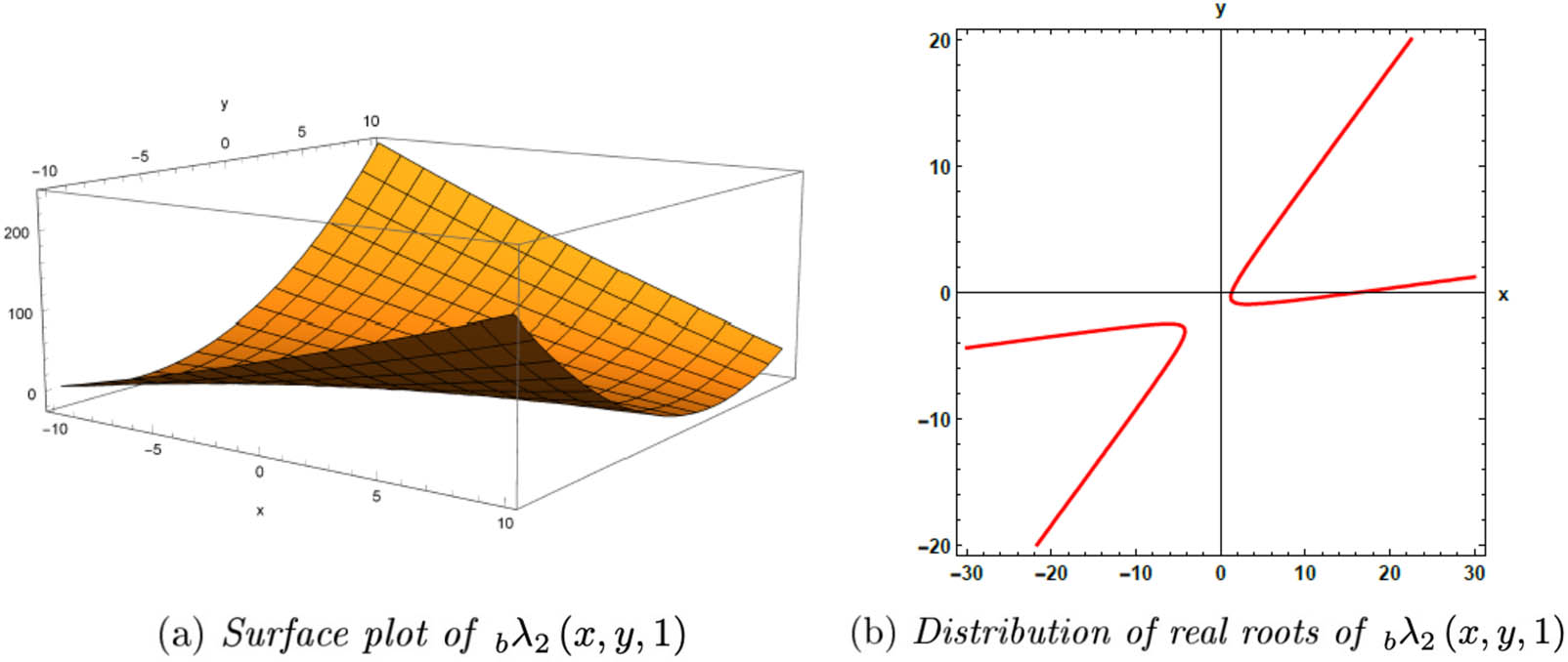
Figures related to
The 3D surface plots of the generalization of second kind Bernoulli-
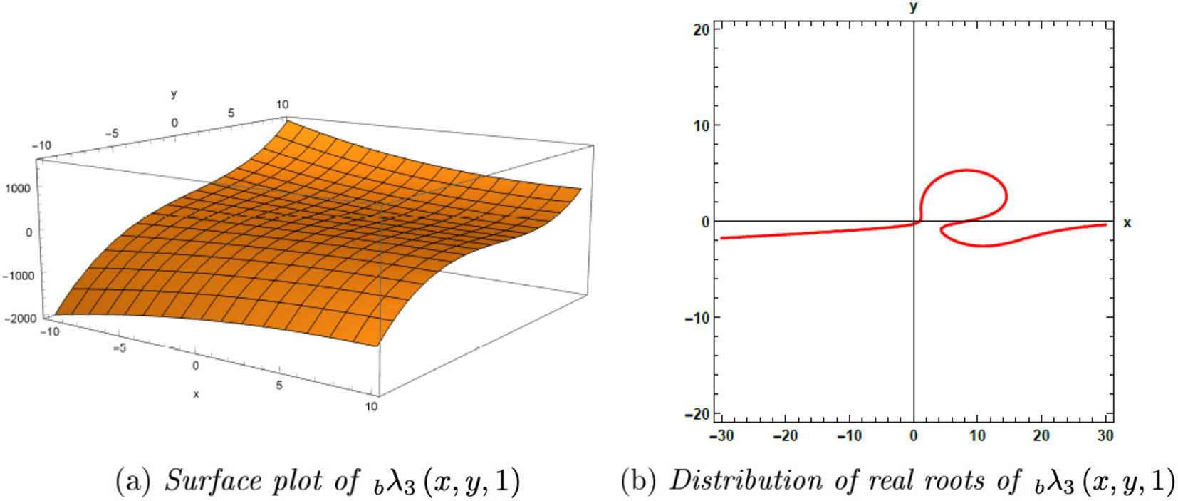
Figures related to
3.2 Generalization of Laguerre-
λ
polynomials
The generalization of Laguerre-
where
Corollary 3.3
The generalization of Laguerre-
and differential equation
Corollary 3.4
The generalization of Laguerre-
The 3D surface plots of the generalization of Laguerre-
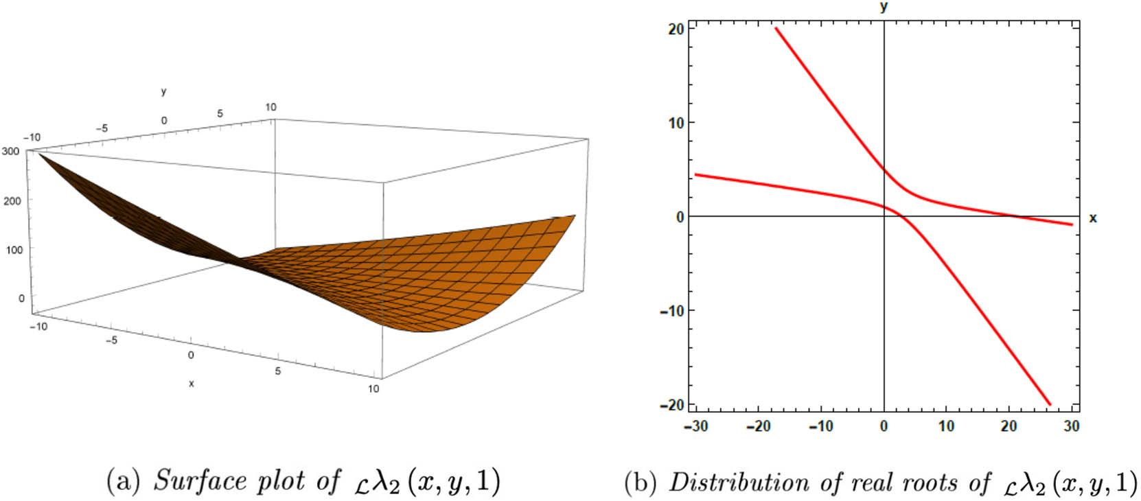
Figures related to
The 3D surface plots of the generalization of Laguerre-
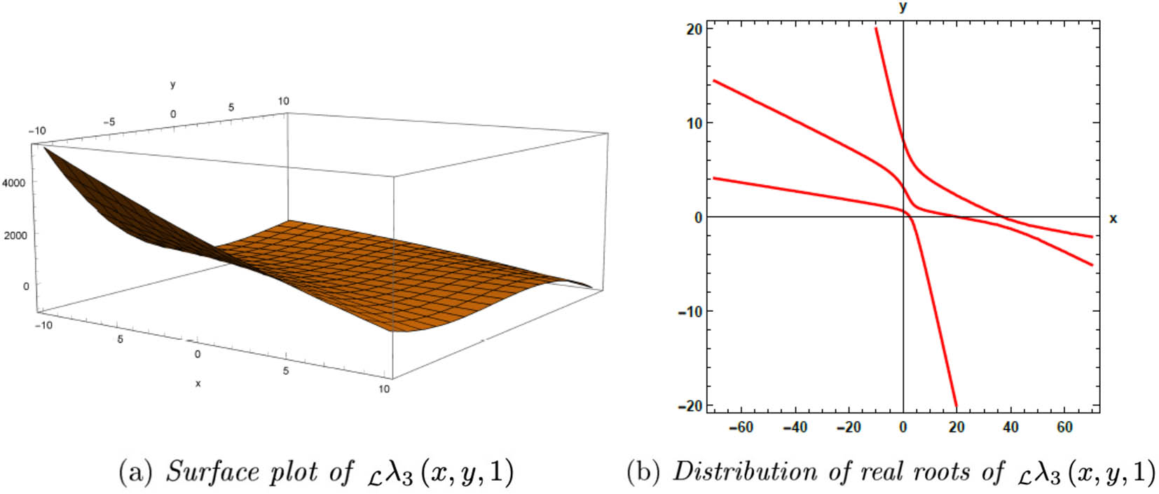
Figures related to
4 Twice-iterated Sheffer-
λ
polynomials
In this section, we replace
Definition 4.1
The twice-iterated Sheffer-
where
and
Corollary 4.1
The twice-iterated Sheffer-
Corollary 4.2
The twice-iterated Sheffer-
or
Corollary 4.3
The twice-iterated Sheffer-
Corollary 4.4
The differential equation of the twice-iterated Sheffer-
Corollary 4.5
The twice-iterated Sheffer-
where
5 Examples
In this part, we introduce the twice-iterated second kind Bernoulli-
5.1 Twice-iterated second kind Bernoulli-
λ
polynomials
The twice-iterated second kind Bernoulli-
where
Corollary 5.1
The twice-iterated second kind Bernoulli-
and differential equation
Corollary 5.2
The twice-iterated second kind Bernoulli-
The 3D surface plots of twice-iterated second kind Bernoulli-
![Figure 5
Figures related to
λ
2
[
2
]
b
(
x
,
y
)
{}_{b}\lambda _{2}^{{[}2]}(x,y)
.](/document/doi/10.1515/dema-2025-0154/asset/graphic/j_dema-2025-0154_fig_005.jpg)
Figures related to
The 3D surface plots of twice-iterated second kind Bernoulli-
![Figure 6
Figures related to
λ
3
[
2
]
b
(
x
,
y
)
{}_{b}\lambda _{3}^{{[}2]}(x,y)
.](/document/doi/10.1515/dema-2025-0154/asset/graphic/j_dema-2025-0154_fig_006.jpg)
Figures related to
5.2 Twice-iterated Laguerre-
λ
polynomials
The twice-iterated Laguerre-
where
Corollary 5.3
The twice-iterated Laguerre-
and differential equation
Corollary 5.4
The twice-iterated Laguerre-
The 3D surface plots of twice-iterated Laguerre-
![Figure 7
Figures related to
λ
2
[
2
]
ℒ
(
x
,
y
)
{}_{{\mathcal{ {\mathcal L} }}}\lambda _{2}^{\left[2]}(x,y)
.](/document/doi/10.1515/dema-2025-0154/asset/graphic/j_dema-2025-0154_fig_007.jpg)
Figures related to
The 3D surface plots of twice-iterated Laguerre-
![Figure 8
Figures related to
λ
3
[
2
]
ℒ
(
x
,
y
)
{}_{{\mathcal{ {\mathcal L} }}}\lambda _{3}^{\left[2]}(x,y)
.](/document/doi/10.1515/dema-2025-0154/asset/graphic/j_dema-2025-0154_fig_008.jpg)
Figures related to
6 Conclusion
In this work, we introduce a new generalization of Sheffer-
Acknowledgments
We would like to thank The Scientific and Technological Research Council of Türkiye (TÜBİTAK) for the TÜBİTAK BİDEB 2211-A General Domestic Doctorate Scholarship Program that supported the first author. We would like to thank the editor and reviewers for their valuable suggestions and comments.
-
Funding information: Authors state no funding involved.
-
Author contributions: All authors have contributed equally to this work.
-
Conflict of interest: Authors state no conflict of interest.
-
Ethical approval: Not applicable.
-
Data availability statement: Data sharing is not applicable as no datasets were generated or used in this study.
References
[1] I. M. Sheffer, Some properties of polynomial sets of type zero, Duke Math. J. 5 (1939), no. 3, 590–622. 10.1215/S0012-7094-39-00549-1Search in Google Scholar
[2] E. D. Rainville, Special Functions, Chelsea Publ., New York, 1971. Search in Google Scholar
[3] S. Roman, The Umbral Calculus, Pure and Applied Mathematics, Academic Press, New York, 1984. Search in Google Scholar
[4] G. Dattoli, Hermite-Bessel and Laguerre-Bessel functions: A by-product of the monomiality principle, Adv. Spec. Funct. Appl. 1 (1999), 147–164. Search in Google Scholar
[5] S. Khan, M. W. Al-Saad, and R. Khan, Laguerre-based Appell polynomials: properties and applications, Math. Comput. Modelling 52 (2010), no. 1–2, 247–259, DOI: https://doi.org/10.1016/j.mcm.2010.02.022. 10.1016/j.mcm.2010.02.022Search in Google Scholar
[6] S. Khan and N. Raza, General-Appell polynomials within the context of monomiality principle, Int. J. Anal. 2013 (2013), no. 1, 328032, DOI: https://doi.org/10.1155/2013/328032. 10.1155/2013/328032Search in Google Scholar
[7] S. Khan, G. Yasmin, R. Khan, and N. A. M. Hassan, Hermite-based Appell polynomials: properties and applications, J. Math. Anal. Appl. 351 (2009), no. 2, 756–764, DOI: https://doi.org/10.1016/j.jmaa.2008.11.002. 10.1016/j.jmaa.2008.11.002Search in Google Scholar
[8] G. Dattoli, M. Migliorati, and H. M. Srivastava, Sheffer polynomials, monomiality principle, algebraic methods and the theory of classical polynomials, Math. Comput. Model. 45 (2007), no. 9–10, 1033–1041, DOI: https://doi.org/10.1016/j.mcm.2006.08.010. 10.1016/j.mcm.2006.08.010Search in Google Scholar
[9] K. A. Penson, P. Blasiak, G. Dattoli, G. H. E. Duchamp, A. Horzela, and A. I. Solomon, Monomiality principle, Sheffer type polynomials and the normal ordering problem, J. Phys. Conf. Ser. 30 (2006), no. 1, 86, DOI: https://doi.org/10.48550/arXiv.quant-ph/0510079. 10.1088/1742-6596/30/1/012Search in Google Scholar
[10] S. Khan and N. Raza, Monomiality principle, operational methods and family of Laguerre-Sheffer polynomials, J. Math. Anal. Appl. 387 (2012), no. 1, 90–102, DOI: https://doi.org/10.1016/j.jmaa.2011.08.064. 10.1016/j.jmaa.2011.08.064Search in Google Scholar
[11] J. F. Steffensen, The poweroid, an extension of the mathematical notion of power, Acta Math. 73 (1941), 333–366. 10.1007/BF02392231Search in Google Scholar
[12] N. Alam, W. A. Khan, C. Kızılateş, and C. S. Ryoo, Two-variable q-general-Appell polynomials within the context of the monomiality principle, Mathematics 13 (2025), no. 5, 765, DOI: https://doi.org/10.3390/math13050765. 10.3390/math13050765Search in Google Scholar
[13] S. Díaz, W. Ramírez, C. Cesarano, J. Hernández, and E. C. P. Rodriguez, The monomiality principle applied to extensions of Apostol-type Hermite polynomials, Eur. J. Pure Appl. Math. 18 (2025), no. 1, 1–17, DOI: https://doi.org/10.29020/nybg.ejpam.v18i1.5656. 10.29020/nybg.ejpam.v18i1.5656Search in Google Scholar
[14] N. Raza, M. Fadel, and S. Khan, On monomiality property of q-Gould-Hopper-Appell polynomials, Arab J. Basic Appl. Sci. 32 (2025), no. 1, 21–29, DOI: https://doi.org/10.1080/25765299.2025.2457206. 10.1080/25765299.2025.2457206Search in Google Scholar
[15] N. Ahmad and W. A. Khan, A new generalization of q-Laguerre-based Appell polynomials and quasi-monomiality, Symmetry 17 (2025), no. 3, 439, DOI: https://doi.org/10.3390/sym17030439. 10.3390/sym17030439Search in Google Scholar
[16] G. Dattoli, E. DiPalma, S. Licciardi, and E. Sabia, From circular to Bessel functions: a transition through the umbral method, Fractal Fract. 1 (2017), no. 1, 9, DOI: https://doi.org/10.3390/fractalfract1010009. 10.3390/fractalfract1010009Search in Google Scholar
[17] S. Khan and M. Haneef, Properties and applications of Sheffer based λ-polynomials, Bol. Soc. Mat. Mex. 30 (2024), no. 1, 9, DOI: https://doi.org/10.1007/s40590-023-00584-2. 10.1007/s40590-023-00584-2Search in Google Scholar
[18] S. Khan and N. Raza, 2-iterated Appell polynomials and related numbers, Appl. Math. Comput. 219 (2013), no. 17, 9469–9483, DOI: https://doi.org/10.1016/j.amc.2013.03.082. 10.1016/j.amc.2013.03.082Search in Google Scholar
[19] H. M. Srivastava, M. A. Ozarslan, and B. Y. Yaşar, Difference equations for a class of twice-iterated Δh-Appell sequences of polynomials, Rev. Real Acad. Cienc. Exactas Fís. Nat. Ser. A Mat. 113 (2019), no. 3, 1851–1871, DOI: https://doi.org/10.1007/s13398-018-0582-0. 10.1007/s13398-018-0582-0Search in Google Scholar
[20] Z. Özat, M. A. Özarslan, and B. Çekim, On Bell based Appell polynomials, Turk. J. Math. 47 (2023), no. 4, 1099–1128, DOI: https://doi.org/10.55730/1300-0098.3415. 10.55730/1300-0098.3415Search in Google Scholar
© 2025 the author(s), published by De Gruyter
This work is licensed under the Creative Commons Attribution 4.0 International License.
Articles in the same Issue
- Research Articles
- On approximation by Stancu variant of Bernstein-Durrmeyer-type operators in movable compact disks
- Circular n,m-rung orthopair fuzzy sets and their applications in multicriteria decision-making
- Grand Triebel-Lizorkin-Morrey spaces
- Coefficient estimates and Fekete-Szegö problem for some classes of univalent functions generalized to a complex order
- Proofs of two conjectures involving sums of normalized Narayana numbers
- On the Laguerre polynomial approximation errors and lower type of entire functions of irregular growth
- New convolutions for the Hartley integral transform imbedded in the Banach algebras and convolution-type integral equations
- Some inequalities for rational function with prescribed poles and restricted zeros
- Lucas difference sequence spaces defined by Orlicz function in 2-normed spaces
- Evaluating the efficacy of fuzzy Bayesian networks for financial risk assessment
- Fixed point results for contractions of polynomial type
- Estimation for spatial semi-functional partial linear regression model with missing response at random
- Investigating the controllability of differential systems with nonlinear fractional delays, characterized by the order 0 < η ≤ 1 < ζ ≤ 2
- New forms of bilateral inequalities for K-g-frames
- Rate of pole detection using Padé approximants to polynomial expansions
- Existence results for nonhomogeneous Choquard equation involving p-biharmonic operator and critical growth
- Note on the shape-preservation of a new class of Kantorovich-type operators via divided differences
- Geršhgorin-type theorems for Z1-eigenvalues of tensors with applications
- New topologies derived from the old one via operators
- Blow up solutions for two-dimensional semilinear elliptic problem of Liouville type with nonlinear gradient terms
- Infinitely many normalized solutions for Schrödinger equations with local sublinear nonlinearity
- Nonparametric expectile shortfall regression for functional data
- Advancing analytical solutions: Novel wave insights and methodologies for beta fractional Kuralay-II equations
- A generalized p-Laplacian problem with parameters
- A study of solutions for several classes of systems of complex nonlinear partial differential difference equations in ℂ2
- Towards finding equalities involving mixed products of the Moore-Penrose and group inverses by matrix rank methodology
-
- Coefficient functionals for Sakaguchi-type-Starlike functions subordinated to the three-leaf function
- Solutions of several general quadratic partial differential-difference equations in ℂ2
- Inequalities for the generalized trigonometric functions with respect to weighted power mean
- Optimization of Lagrange problem with higher-order differential inclusion and special boundary-value conditions
- Hankel determinants for q-starlike functions connected with q-sine function
- System of partial differential hemivariational inequalities involving nonlocal boundary conditions
- A new family of multivalent functions defined by certain forms of the quantum integral operator
- A matrix approach to compare BLUEs under a linear regression model and its two competing restricted models with applications
- Weighted composition operators on bicomplex Lorentz spaces with their characterization and properties
- Behavior of spatial curves under different transformations in Euclidean 4-space
- Commutators for the maximal and sharp functions with weighted Lipschitz functions on weighted Morrey spaces
- A new kind of Durrmeyer-Stancu-type operators
- A study of generalized Mittag-Leffler-type function of arbitrary order
- On the approximation of Kantorovich-type Szàsz-Charlier operators
- Split quaternion Fourier transforms for two-dimensional real invariant field
- Quantum injectivity of G-frames in Hilbert spaces
- Some results on disjointly weakly compact sets
- On Motzkin sequence spaces via q-analog and compact operators
- Existence and multiplicity of nontrivial solutions for Schrödinger-Bopp-Podolsky systems with critical nonlinearity in ℝ3
- Stability analysis of linear time-invariant difference-differential system with constant and distributed delays
- The discriminant of quasi m-boundary singularities
- Norm constrained empirical portfolio optimization with stochastic dominance: Robust optimization non-asymptotics
- Fuzzy stability of multi-additive mappings
- On inequalities involving n-polynomial exponential-type convex functions
- Review Article
- Characterization generalized derivations of tensor products of nonassociative algebras
- Special Issue on Differential Equations and Numerical Analysis - Part II
- Existence and optimal control of Hilfer fractional evolution equations
- Persistence of a unique periodic wave train in convecting shallow water fluid
- Existence results for critical growth Kohn-Laplace equations with jumping nonlinearities
- Monotonicity and oscillation for fractional differential equations with Riemann-Liouville derivatives
- Nontrivial solutions for a generalized poly-Laplacian system on finite graphs
- Stability and bifurcation analysis of a modified chemostat model
- Special Issue on Nonlinear Evolution Equations and Their Applications - Part II
- Analytic solutions of a generalized complex multi-dimensional system with fractional order
- Extraction of soliton solutions and Painlevé test for fractional Peyrard-Bishop DNA model
- Special Issue on Recent Developments in Fixed-Point Theory and Applications - Part II
- Some fixed point results with the vector degree of nondensifiability in generalized Banach spaces and application on coupled Caputo fractional delay differential equations
- On the sum form functional equation related to diversity index
- Special Issue on International E-Conference on Mathematical and Statistical Sciences - Part II
- Simpson, midpoint, and trapezoid-type inequalities for multiplicatively s-convex functions
- Converses of nabla Pachpatte-type dynamic inequalities on arbitrary time scales
- Special Issue on Blow-up Phenomena in Nonlinear Equations of Mathematical Physics - Part II
- Energy decay of a coupled system involving a biharmonic Schrödinger equation with an internal fractional damping
- Special Issue on Some Integral Inequalities, Integral Equations, and Applications - Part II
- Nonlinear heat equation with viscoelastic term: Global existence and blowup in finite time
- New Jensen's bounds for HA-convex mappings with applications to Shannon entropy
- Special Issue on Approximation Theory and Special Functions 2024 conference
- Ulam-type stability for Caputo-type fractional delay differential equations
- Faster approximation to multivariate functions by combined Bernstein-Taylor operators
- (λ, ψ)-Bernstein-Kantorovich operators
- Some special functions and cylindrical diffusion equation on α-time scale
- (q, p)-Mixing Bloch maps
- Orthogonalizing q-Bernoulli polynomials
- On better approximation order for the max-product Meyer-König and Zeller operator
- Moment-based approximation for a renewal reward process with generalized gamma-distributed interference of chance
- A note on linear compositions of the Mellin convolution operators in the weighted Mellin-Lebesgue spaces
- A new perspective on generalized Laguerre polynomials
- Global existence of semilinear system of Klein-Gordon equations in anti-de Sitter spacetime
- Estimates for Durrmeyer-type exponential sampling series in Mellin-Orlicz spaces
- ℐ-αβ-statistical relative uniform convergence for double sequences and its applications
- New developments for the Jacobi polynomials
- Generalization of Sheffer-λ polynomials
- Special Issue on Variational Methods and Nonlinear PDEs
- A note on mean field type equations
- Ground states for fractional Kirchhoff double-phase problem with logarithmic nonlinearity
- Solution of nonlinear Langevin equations involving Hilfer-Hadamard fractional order derivatives and variable coefficients
- Bifurcation, quasi-periodic, and wave solutions to the fractional model of optical fibers in communication systems
- Multiplicity and concentration behavior of solutions for the generalized quasilinear Schrödinger equation with critical growth