
Nearest Neighbour Particle-Particle Interaction in Fermionic Quasi One-Dimensional Flat Band Lattices
-
Simon Tilleke


Abstract
In this paper, we have studied spinless fermions in four specific quasi one-dimensional systems that are known to host flat bands in the noninteracting limit: the triangle lattice, the stub lattice, the diamond lattice, and the diamond lattice with transverse hopping. The influence of the nearest neighbour interaction on the flat bands was investigated. We used exact diagonalization of finite size lattices employing the Lanczos technique and determine the single particle spectral functions of the interacting system. Our results are compared with mean field calculations. In the cases of the triangle lattice and the stub lattice we found that the flat bands become dispersive in the presence of a finite interaction. For the diamond lattice and the diamond lattice with transverse hopping, we demonstrated that the flat bands are robust under the influence of the interaction in certain parameter ranges. Such systems could be realised experimentally with cold atoms in optical lattices.
1 Introduction
Recently there has been an increased interest in flat band lattice systems. Such systems are characterised by the presence of completely dispersionless energy bands, which are accompanied by a macroscopic degeneracy, zero group velocity, and infinite effective mass. They also possess a macroscopic number of degenerate localised energy eigenstates. Flat bands appear in a variety of condensed matter systems [1], like the Landau levels of an electron gas, frustrated magnets [2], edge states of graphene [3], topological insulators [4], Weyl semimetals [5], unconventional superconductors [6], or optical lattices [7]. They can also emerge in strongly correlated electron systems [8]. Flat bands have been realised experimentally with photonic waveguide arrays [9], [10], exciton-polariton condensates [11], [12], cold atoms [13], [14], and on an appropriately doped Cu surface [15].
In a flat band system the influence of perturbations to the system like disorder or interactions can lead to interesting new phenomena. For example, interactions can lead to ferromagnetism [16], [17], topological magnons [18], [19], a fractional quantum Hall state [20], [21], [22], spin liquid states [23], or surface superconductivity with high critical temperature [24]. Disorder in flat band systems can give rise to an inverse Anderson transition (delocalization transition) [25], multifractal behaviour [26], or mobility edges with algebraic singularities [27]. However, most of these perturbations lift the degeneracy of the flat band.
In the present work we have studied several quasi one-dimensional flat band systems and ask whether the flat bands remain robust in the presence of an interaction between the particles. We show that in specific cases the flat band stays flat even in the presence of interaction. Such systems can be useful for information storage and also they might show many body localisation [28], [29], [30], because they possess stationary localised states in the presence of interaction. We restricted ourselves to spinless fermions on the quasi one-dimensional lattices shown in Figure 1. These lattices were shown to host flat bands previously [31]. We considered a nearest neighbour repulsive interaction between the particles. To determine the behaviour of these systems in the presence of interaction we performed numerical exact diagonalization of the many body Hamiltonian using the Lanczos technique. We compared these calculations with mean field calculations, which agree very well, when the interaction strength is weak.
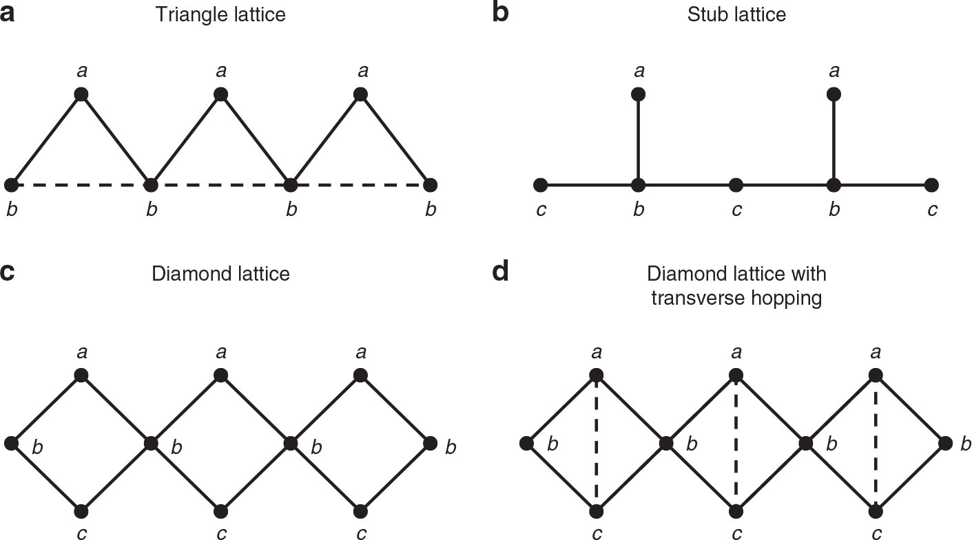
Quasi one-dimensional lattices considered in this work: (a) triangle lattice, (b) stub lattice, (c) diamond lattice, and (d) diamond lattice with transverse hopping. The nearest neighbour hopping parameter t is denoted by solid lines in the lattices. The dashed lines correspond to a next nearest neighbour hopping parameter t′. The triangle lattice (a) possesses a flat band, when
2 Models and Calculations
We investigated a tight-binding model having one fermionic state per lattice site. Hopping up to the next nearest neighbour is included, as shown in Figure 1. In addition, a nearest neighbour interaction acts between the particles. The Hamiltonian is given by
where
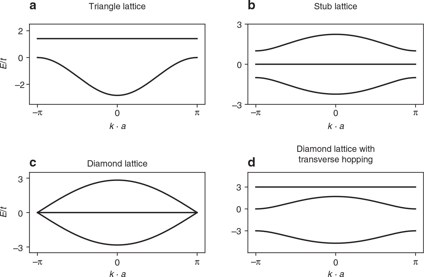
In Figure 2 we show the bare band structures corresponding to the lattices in Figure 1. All energies are given in units of the nearest neighbour hopping t. The triangle lattice in Figure 2a has two bands. The higher energy band becomes flat, when
2.1 Mean Field Calculations
As a comparison with exact calculations a mean field approximation to the Hamiltonian (1) is useful. As we will see below, the mean-field approximation is a good approximation only for weak interaction strengths. However, it is simpler to calculate and serves as a reference. We look for homogeneous solutions, such that the ground state expectation value of the particle number operator
where E0 is a constant energy offset
Here,
where the sum runs over all neighbours of site α.
Within the mean field approximation the Hamiltonian HMF describes a system of noninteracting fermions and can be diagonalised by transformation into momentum space. This way it can be brought into the form
where
where
These solutions are determined iteratively, i.e. one starts with a reasonable guess for nβ, calculates
2.2 Exact Calculations Using the Lanczos Procedure
In an interacting many particle system, a band structure in the strict sense does not exist anymore. However, we can still examine the single particle excitations above the ground state of an interacting many particle system and ask whether they possess flat bands in the sense that the excitation energy is independent of momentum. For this purpose we calculated the single particle spectral function and looked for flat band structures.
To find the ground state of the system we used the Lanczos procedure [32]. In the Lanczos procedure one starts with a normalised random state vector and constructs an orthonormal basis by repeatedly applying the Hamiltonian. Within this basis the Hamiltonian is of tridiagonal form. After NL steps one obtains an
In the presence of a flat band, the ground state of the Hamiltonian can be highly degenerate. For a noninteracting system this becomes clear from the bandstructures in Figure 2: if the band filling is chosen such that the flat band is only partially occupied, the particles in the flat band can be rearranged without changing the energy of the system. For this reason it is of interest here to also determine the degeneracy of the ground state. This can be done with the Lanczos procedure in the following way: after a ground state has been determined from a random start vector, the Lanczos procedure is repeated with a different random start vector. If the new ground state is linearly independent from the first ground state, the Lanczos procedure is repeated again until no new linearly independent ground state is found anymore. Technically, after each Lanczos run, one determines the rank of the matrix of all ground states found so far. If the rank does not change anymore, the procedure can be stopped.
2.3 Spectral Functions
The single particle spectral function
We first determine the ground state
Note, that the state
Here, EG is the ground state energy of the M particle system (before the particle was removed or added) and Γ is a broadening parameter which helps to visualise the spectral function and is taken to be Γ = 0.05 here. The function
3 Results
In this section our results for the mean field bandstructure and the spectral function (11) are presented for the triangle lattice, stub lattice, and diamond lattices shown in Figure 1. In all cases the bandfilling was chosen in such a way that the flat band is half filled in the noninteracting case V = 0. In most cases a few hundred Lanczos iterations were sufficient to obtain accurate ground states and spectral functions.
3.1 Triangle Lattice
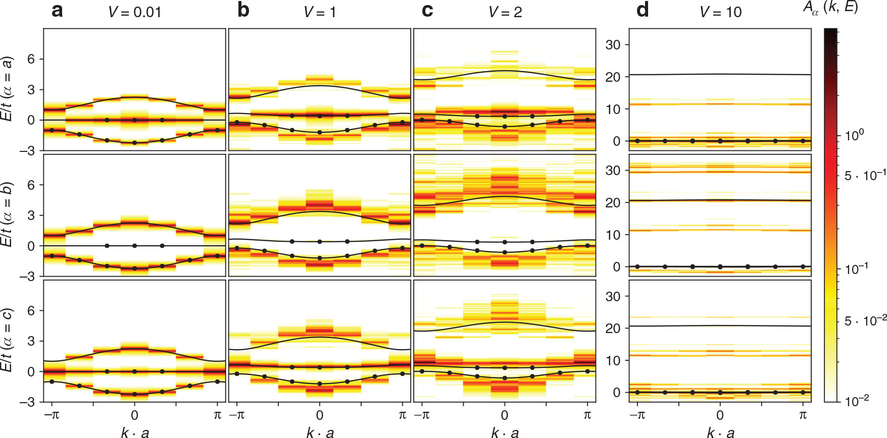
In this section the triangle lattice from Figure 1a with
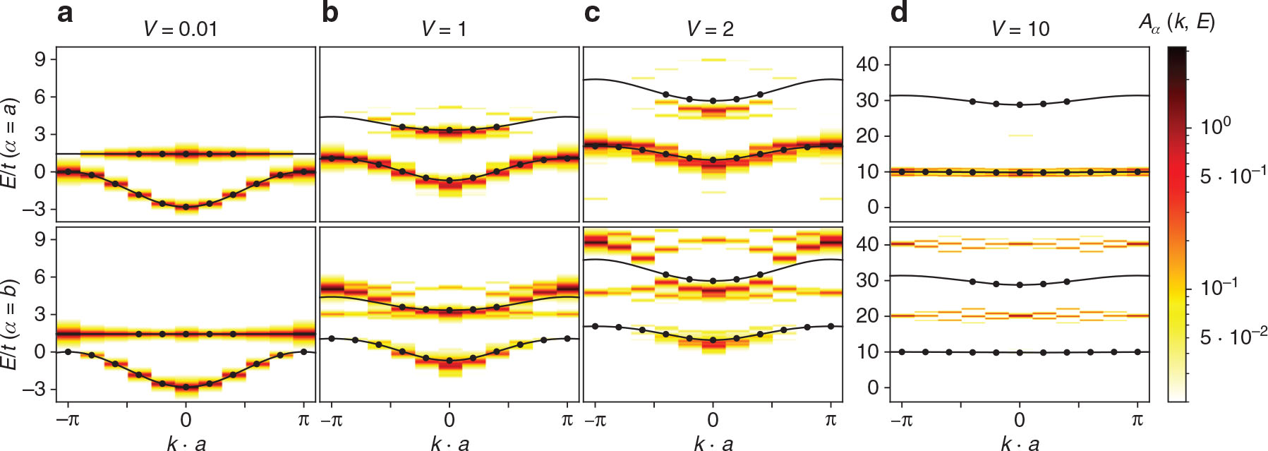
Spectral functions
The mean field band structures and spectral functions
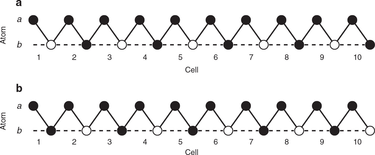
The two leading real space basis states that contribute most to the ground state wave function of the triangular lattice for V ≳ 10. In both states the a sites are fully occupied. In (a) the even numbered b sites are occupied, while in (b) the even numbered b sites are empty.
Spectral functions
To verify this qualitative picture we expanded the ground state wave function into the real space basis states. For large positive interaction strength V ≳ 10 it turns out that the ground state is essentially just a linear superposition of the two real space eigenstates shown in Figure 4. For V = 10 we found that both states contributed 46.9 % each to the ground state wave function. For V = 100 they even contributed 49.96 % each.
To summarise, for the triangular lattice the flat band becomes dispersive as soon as a repulsive nearest neighbour interaction is turned on. In the limit of strong interaction at three quarter filling, however, the interaction can block the motion of the particles and all bands become flat again.
3.2 Stub Lattice
In this section the stub lattice from Figure 1b is studied. We considered six unit cells filled with nine particles, such that in the noninteracting case the lower dispersive band is fully filled, the flat band is half filled, and the upper dispersive band is empty.
The mean field band structures and spectral functions
Spectral functions
3.3 Diamond Lattice
In contrast to the triangle lattice and stub lattice, the diamond lattice possesses an additional mirror symmetry with respect to the main axis of the lattice. Thus, all energy eigenstates can be chosen as symmetric or antisymmetric states with respect to this axis. For this reason it is useful to define the following annihilation operators:
and
and calculate the corresponding spectral functions
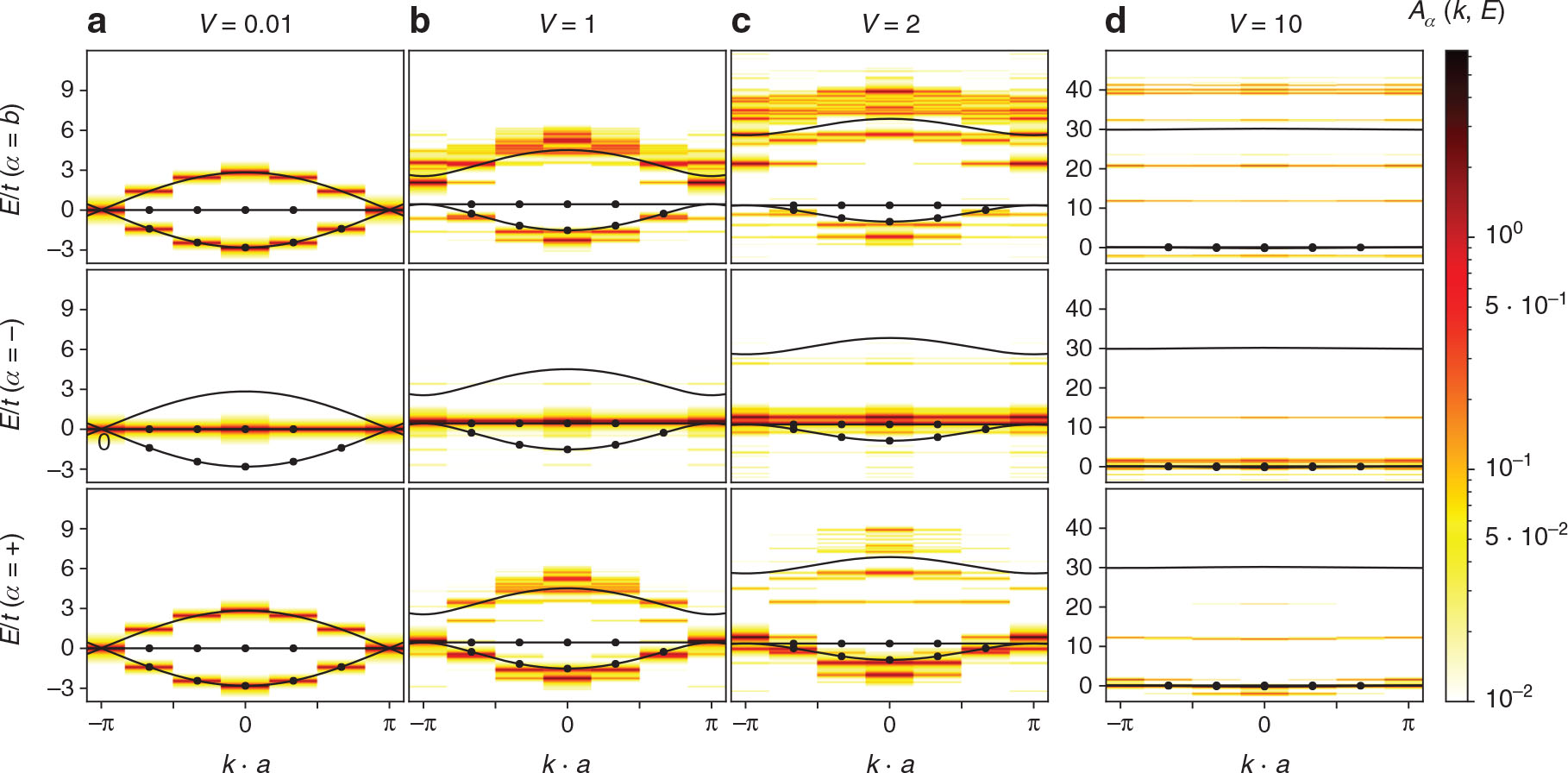
The mean field band structures and spectral functions
Spectral functions and mean field bandstructures for the diamond lattice with next nearest neighbour hopping
As is seen in Figure 6 the flat band appears in the α = − channel and thus corresponds to those states that possess antisymmetric wave functions with respect to the mirror axis. The two dispersive bands appear to be linear combinations of the b and + channels. For V ≲ 1 the flat band remains flat in both mean field solution and spectral function. For V ≳ 2 in the exact calculation the flat band starts to split into two flat bands, seen in Figure 6c and d. In the strongly interacting limit V ≫ 1 the b sites become unfavourable, because they are connected to four sites each. Thus, the particles predominantly occupy the a and c sites to avoid the repulsion. For this reason the excitations in the b channel appear at much higher energy than in the a and c channels when V becomes large. In this limit all three bands become flat. The b band appears to split into 5 sub-bands at energies
Spectral functions and mean field bandstructures for the diamond lattice with next nearest neighbour hopping
To summarise, for the diamond lattice we found a flat band in the α = − channel that persists throughout the whole range of interaction strengths V. For V ≳ 2 this band starts to split into two separate flat sub-bands. The higher energy sub-band can be interpreted as coming from states with occupied b sites.
3.4 Diamond Lattice with Transverse Hopping
The diamond lattice with transverse hopping and an interaction between the a and c sites possesses the same mirror symmetry as the bare diamond lattice. Therefore the spectral functions for the +, −, and b channels are discussed also in this section.
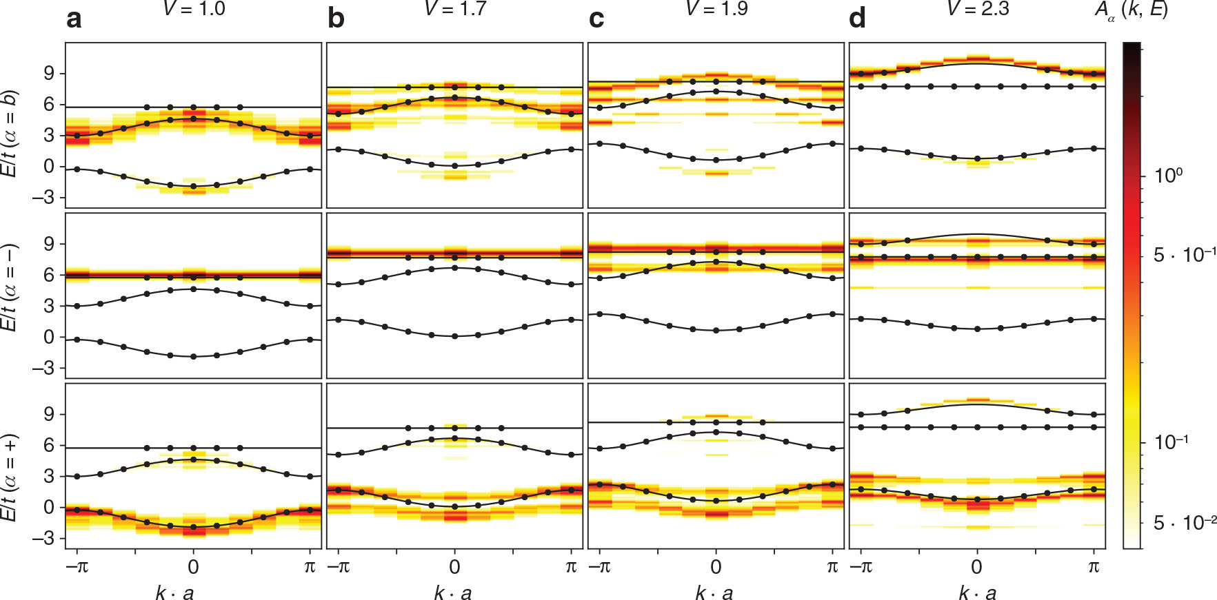
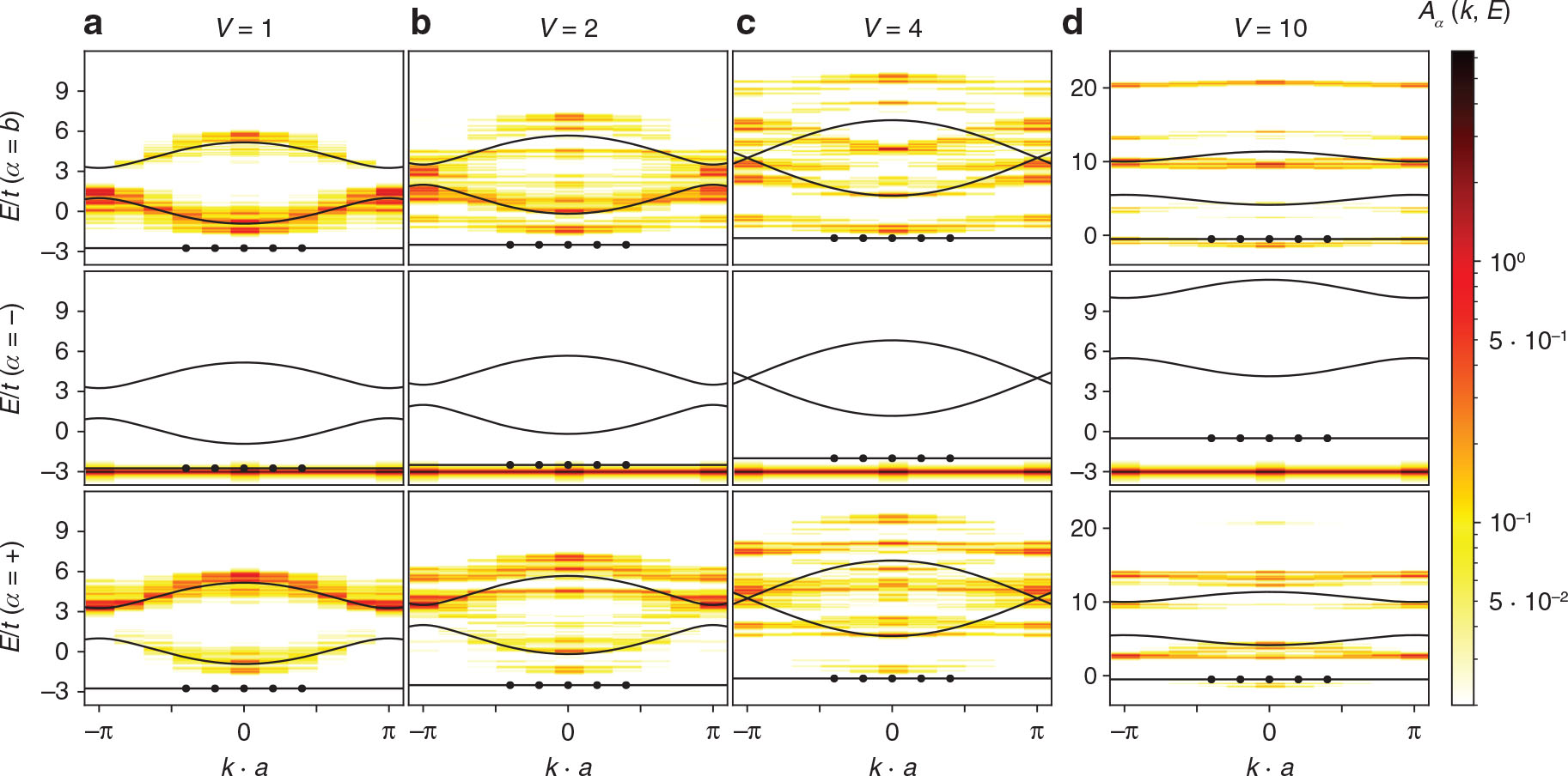
In Figure 7 the spectral functions
In Figure 8 the spectral functions
To summarise, for the diamond lattice with
We have seen that under a finite interaction the flat band does not stay flat for the triangle lattice and stub lattice, while it has a robustness for the two diamond lattices. We suggest that the mirror symmetry of the diamond lattice plays an important role here to stabilise the flat band. The mirror symmetry guarantees the existence of energy eigenstates that are antisymmetric, i.e. have zeroes on the b sites. In such states the particles in different unit cells are effectively decoupled. Then, Wannier states localised in a single unit cell become eigenstates of the Hamiltonian. As a result, the flat band remains flat, even in the presence of interaction.
4 Summary and Conclusions
We have investigated spinless fermions in several quasi one-dimensional lattices that are known to host flat bands in the noninteracting limit. We studied the influence of a repulsive nearest neighbour interaction on the flat bands using both mean field approximation and exact diagonalisation by Lanczos technique.
For the triangle lattice and stub lattice we found that the flat band becomes dispersive, as soon as a finite interaction is turned on. For the three quarter filled triangle lattice the bands become flat again in the strongly interacting limit V → ∞.
For the bare diamond lattice we found that the flat band remains flat for all interaction strengths. For V ≳ 2 the flat band splits into two flat sub-bands. The ground state degeneracy becomes equal to the number of lattice sites as soon as a finite interaction strength is turned on.
For the diamond lattice with transverse hopping
For the diamond lattice with transverse hopping
Generally, for small interaction strengths V ≲ 1 the results from mean field approximation agree well with exact results from the Lanczos technique. For larger interaction strengths the spectral functions appear to be smeared out in energy or show splittings that are not reproduced by mean field approximation.
Acknowledgement
Financial support from the DFG via the research group FOR2692, Funder Id: http://dx.doi.org/10.13039/501100001659, grant number 397171440 is gratefully acknowledged. We would like to thank S. kleine Brüning and S. Kehrein for valuable discussions.
References
[1] D. Leykam, A. Andreanov, and S. Flach, Adv. Phys. X 3, 1473052 (2018).10.1080/23746149.2018.1473052Suche in Google Scholar
[2] O. Derzhko, J. Richter, and M. Maksymenko, Int. J. Mod. Phys. B 29, 1530007 (2015).10.1142/S0217979215300078Suche in Google Scholar
[3] K. Nakada, M. Fujita, G. Dresselhaus, and M. S. Dresselhaus, Phys. Rev. B 54, 17954 (1996).10.1103/PhysRevB.54.17954Suche in Google Scholar PubMed
[4] T. Paananen and T. Dahm, Phys. Rev. B 87, 195447 (2013).10.1103/PhysRevB.87.195447Suche in Google Scholar
[5] T. Paananen, H. Gerber, M. Götte, and T. Dahm, New J. Phys. 16, 033019 (2014).10.1088/1367-2630/16/3/033019Suche in Google Scholar
[6] S. Matsuura, P.-Y. Chang, A. P. Schnyder, and S. Ryu, New J. Phys. 15, 065001 (2013).10.1088/1367-2630/15/6/065001Suche in Google Scholar
[7] T. Paananen and T. Dahm, Phys. Rev. A 91, 033604 (2015).10.1103/PhysRevA.91.033604Suche in Google Scholar
[8] R.-Q. He and Z.-Y. Weng, Sci. Rep. 6, 35208 (2016).10.1038/srep35208Suche in Google Scholar PubMed PubMed Central
[9] R. A. Vicencio, C. Cantillano, L. Morales-Inostroza, B. Real, C. Meja-Cortés, et al., Phys. Rev. Lett. 114, 245503 (2015).10.1103/PhysRevLett.114.245503Suche in Google Scholar PubMed
[10] S. Mukherjee, A. Spracklen, D. Choudhury, N. Goldman, P. Öhberg, et al., Phys. Rev. Lett. 114, 245504 (2015).10.1103/PhysRevLett.114.245504Suche in Google Scholar PubMed
[11] N. Masumoto, N. Y. Kim, T. Byrnes, K. Kusudo, A. Löffler, et al., New J. Phys. 14, 065002 (2012).10.1088/1367-2630/14/6/065002Suche in Google Scholar
[12] F. Baboux, L. Ge, T. Jacqmin, M. Biondi, E. Galopin, et al., Phys. Rev. Lett. 116, 066402 (2016).10.1103/PhysRevLett.116.066402Suche in Google Scholar PubMed
[13] M. Aidelsburger, M. Lohse, C. Schweizer, M. Atala, J. T. Barreiro, et al., Nat. Phys. 11, 162 (2015).10.1038/nphys3171Suche in Google Scholar
[14] S. Taie, H. Ozawa, T. Ichinose, T. Nishio, S. Nakajima, et al., Sci. Adv. 1, e1500854 (2015).10.1126/sciadv.1500854Suche in Google Scholar PubMed PubMed Central
[15] M. R. Slot, T. S. Gardenier, P. H. Jacobse, G. C. P. van Miert, S. N. Kempkes, et al., Nat. Phys. 13, 672 (2017).10.1038/nphys4105Suche in Google Scholar PubMed PubMed Central
[16] H. Tasaki, Phys. Rev. Lett. 69, 1608 (1992).10.1103/PhysRevLett.69.1608Suche in Google Scholar PubMed
[17] J. S. Hofmann, F. F. Assaad, and A. P. Schnyder, Phys. Rev. B 93, 201116 (2016).10.1103/PhysRevB.93.201116Suche in Google Scholar
[18] X.-F. Su, Z.-L. Gu, Z.-Y. Dong, and J.-X. Li, Phys. Rev. B 97, 245111 (2018).10.1103/PhysRevB.97.245111Suche in Google Scholar
[19] X.-F. Su, Z.-L. Gu, Z.-Y. Dong, S.-L. Yu, and J.-X. Li, Phys. Rev. B 99, 014407 (2019).10.1103/PhysRevB.99.014407Suche in Google Scholar
[20] C. Weeks and M. Franz, Phys. Rev. B 85, 041104 (2012).10.1103/PhysRevB.85.041104Suche in Google Scholar
[21] K. Sun, Z. Gu, H. Katsura, and S. Das Sarma, Phys. Rev. Lett. 106, 236803 (2011).10.1103/PhysRevLett.106.236803Suche in Google Scholar PubMed
[22] E. J. Bergholtz and Z. Liu, Int. J. Mod. Phys. B 27, 1330017 (2013).10.1142/S021797921330017XSuche in Google Scholar
[23] S.-H. Lee, C. Broholm, W. Ratcliff, G. Gasparovic, Q. Huang, et al., Nature (London) 418, 856 (2002).10.1038/nature00964Suche in Google Scholar PubMed
[24] N. B. Kopnin, M. Ijäs, A. Harju, and T. T. Heikkilä, Phys. Rev. B 87, 140503 (2013).10.1103/PhysRevB.87.140503Suche in Google Scholar
[25] M. Goda, S. Nishino, and H. Matsuda, Phys. Rev. Lett. 96, 126401 (2006).10.1103/PhysRevLett.96.126401Suche in Google Scholar PubMed
[26] J. T. Chalker, T. S. Pickles, and P. Shukla, Phys. Rev. B 82, 104209 (2010).10.1103/PhysRevB.82.104209Suche in Google Scholar
[27] J. D. Bodyfelt, D. Leykam, C. Danieli, X. Yu, and S. Flach, Phys. Rev. Lett. 113, 236403 (2014).10.1103/PhysRevLett.113.236403Suche in Google Scholar PubMed
[28] R. Nandkishore and D. A. Huse, Annu. Rev. Cond. Mat. Phys. 6, 15 (2015).10.1146/annurev-conmatphys-031214-014726Suche in Google Scholar
[29] Y. Kuno, T. Orito, and I. Ichinose, New J. Phys. 22, 013032 (2020).10.1088/1367-2630/ab6352Suche in Google Scholar
[30] N. Roy, A. Ramachandran, and A. Sharma, arXiv preprint 1912.09951 (2019).Suche in Google Scholar
[31] M. Hyrkäs, V. Apaja, and M. Manninen, Phys. Rev. A 87, 023614 (2013).10.1103/PhysRevA.87.023614Suche in Google Scholar
[32] C. Lanczos, J. Res. Natl. Bur. Stand. 45, 255 (1950).10.6028/jres.045.026Suche in Google Scholar
[33] G. Rickayzen, Green’s Functions and Condensed Matter, Academic Press, London 1987.Suche in Google Scholar
© 2020 Walter de Gruyter GmbH, Berlin/Boston
Artikel in diesem Heft
- Frontmatter
- Geometry of the Rabi Problem and Duality of Loops
- Nearest Neighbour Particle-Particle Interaction in Fermionic Quasi One-Dimensional Flat Band Lattices
- Predicting Imperfect Echo Dynamics in Many-Body Quantum Systems
- Thermalization and Nonequilibrium Steady States in a Few-Atom System
- Selected applications of typicality to real-time dynamics of quantum many-body systems
- Work Statistics and Energy Transitions in Driven Quantum Systems
- Probing Nonexponential Decay in Floquet–Bloch Bands
- Nonequilibrium Transport and Phase Transitions in Driven Diffusion of Interacting Particles
- Finite-Size Scaling of Typicality-Based Estimates
- Modeling the Impact of Hamiltonian Perturbations on Expectation Value Dynamics
- Coherent Transport in Periodically Driven Mesoscopic Conductors: From Scattering Amplitudes to Quantum Thermodynamics