
Integral Laplacian graphs with a unique repeated Laplacian eigenvalue, I
-
Abdul Hameed


Abstract
The set
and completely describe those with
1 Introduction
Let
The study of graphs whose adjacency matrix has integer eigenvalues was probably introduced by Harary and Schwenk [17]. The same kind of problem has been addressed with the eigenvalues of the Laplacian matrix. A graph
Several explicit constructions of Laplacian integral graphs of special types appear in the literature. For example, Merris [22] showed that degree maximal graphs are Laplacian integral, see also [24,26]. A connected class of graphs, namely
One way to describe and study all the integral Laplacian graphs (if any) is to study graphs having certain kinds of Laplacian spectra. Thus, starting with graphs with simple integer Laplacian eigenvalues, one can then consider integral Laplacian graphs with all simple Laplacian eigenvalues excluding one that is repeated. On the next step, it is allowed for graphs to have two Laplacian eigenvalues of multiplicity 2 or a unique multiple eigenvalue of multiplicity 3.
The first step in this scheme was undertaken by Fallat et al. in their work [9] on the integral Laplacian graphs with simple Laplacian eigenvalues.
Definition 1.1
A set
Fallat et al. [9] considered the sets of the form
and found out when such sets are Laplacian realizable and completely described the graphs realizing
Following the aforementioned scheme, in this work, we study Laplacian integral graphs having only one multiple (non-zero) Laplacian eigenvalue whose multiplicity equals exactly 2. Namely, we describe the graphs realizing the multisets of the form
where
The graphs realizing
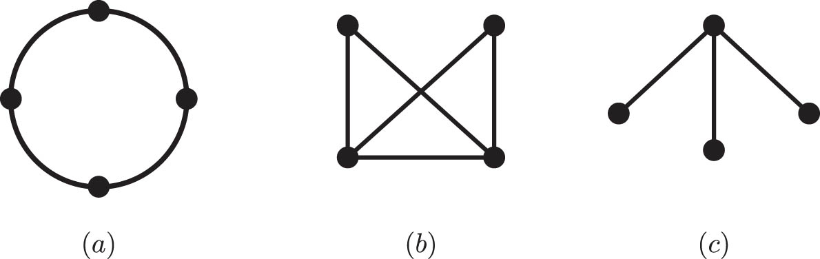
Graph (a), (b), and (c) realizing
Note that the graphs (b) and (c) in Figure 1 are threshold, see, e.g., [22,25]. The explicit constructions of graphs realizing
Laplacian integral graphs realizing
| Construction | Laplacian spectrum |
|
|---|---|---|
|
|
|
|
|
|
|
|
|
|
|
|
Laplacian integral graphs realizing
| Construction | Laplacian spectrum |
|
|---|---|---|
|
|
|
|
|
|
|
|
|
|
|
|
|
|
|
|
|
|
|
|
Laplacian integral graphs that realizing
| Graph | Lapl. Spectrum |
|
Graph | Lapl. Spectrum |
|
|---|---|---|---|---|---|
|
|
|
|
|
|
|
|
|
|
|
|
|
|
|
|
|
|
|
|
|
|
|
|
|
|
|
|
|
|
|
|
|
|
|
In this study, we consider graphs realizing
As mentioned above, for
Graph
Graph
However, there are no other Laplacian realizable multisets
The article is organized as follows: in Section 2, we list basic definitions and notations; several important results that we use in our work are stated in Section 3: where we also prove some auxiliary statements and theorems; in Sections 4 and 5, we list all the Laplacian realizable multisets of the form
2 Preliminaries
Let
Definition 2.1
Given two graphs
Definition 2.2
The Cartesian product of the graphs
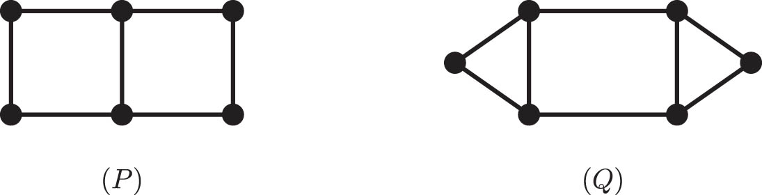
The ladder graph is an example of a graph which is obtained from the Cartesian product of two path graphs:
We denote the eigenvalues of the Laplacian matrix
It is well known that
Proposition 2.3
Let G be a simple graph on n vertices. Then,
The Laplacian spectrum of the graph operations mentioned above is related to the Laplacian spectra of the initial graphs. Thus, the Laplacian spectrum of
Theorem 2.4
Let G be a graph with n vertices. If
The spectrum of the join of two graphs was obtained by Kel’mans [18] in terms of the characteristic polynomials of Laplacian matrices. The following form of Kel’mans’ theorem can be found, e.g., in the study by Merris [26].
Theorem 2.5
Let G and H be two graphs of order n and m, respectively, whose eigenvalues are as follows:
Then, the Laplacian spectrum of the join
Note that the eigenvalues here are not in increasing order.
As one can see from equation (3), the order of the join of two graphs is a Laplacian eigenvalue of the join. It turns out that this fact is a necessary and sufficient condition for a graph to be a join, see, e.g., [27].
Theorem 2.6
Let G be a connected graph of order n. Then, n is a Laplacian eigenvalue of G if and only if G is the join of two graphs.
The Laplacian spectrum of the Cartesian product of two graphs is given in the following theorem, see, e.g., [23].
Theorem 2.7
Let F and H be graphs having spectrum,
then the Laplacian spectrum of the Cartesian product of F and H is
From equation (4), it is easy to see that the Laplacian spectrum of the Cartesian product of two Laplacian integral graphs is Laplacian integral.
As we mentioned in Introduction, the graphs whose Laplacian spectra are of the form
Proposition 2.8
If
If
If
If
Proposition 2.9
Suppose that
Proposition 2.10
Suppose that
Proposition 2.11
Suppose that
Proposition 2.8 completely resolves the existence of graphs realizing the spectrum
3 Laplacian spectral properties of the join of graphs and auxiliary properties of multisets
S
{
i
,
j
}
n
m
Theorem 2.6 characterizes graphs with the largest Laplacian eigenvalue equal to the order of the graphs. However, if the order of the graph is a repeated eigenvalue, then we can obtain more information about the structure as well as spectrum of the corresponding graph.
Theorem 3.1
Let G be a connected graph of order n, and let n be a Laplacian eigenvalue of G of multiplicity 2. Then,
Proof
Since
Let us denote the Laplacian spectra of the graphs
Then, by Theorem 2.5, the Laplacian spectrum of
Here, the eigenvalues are not in increasing order.
Since the graph
Now, from equation (6), we obtain that
Since the graph
On the contrary, the following theorem provides a necessary and sufficient condition on a graph
Theorem 3.2
Let a graph G be a join. The number 1 is a Laplacian eigenvalue of G if and only if
Proof
Let
If both the numbers
Thus, we have that one of the numbers
Conversely, let
Now we are in a position to establish a few general facts on the realizability of multisets
Lemma 3.3
Suppose that
for
for
Proof
If a graph
Here,
Now if
The following lemma is of frequent use in the sequel.
Lemma 3.4
Let
Proof
By Theorem 2.5, one easily obtains that if a graph
Remark 3.5
Note that the converse statement of Lemma 3.4 does not hold, in general. For instance, from Table A2 in Appendix A, it follows that the multiset
We conclude this section with the following theorem.
Theorem 3.6
Let G realize
Proof
Let
Thus, the graphs
Indeed, if
If
Thus, if a graph
Remark 3.7
For
4 Graphs realizing the multisets
S
{
i
,
j
}
n
n
In this section, we describe the graphs realizing the multisets
Thus, we come to the following lemma (cf. [9, Lemma 2.5]).
Lemma 4.1
If the multiset
Now we are in a position to describe all the Laplacian realizable multisets
Theorem 4.2
Suppose
If
If
If
If
Proof
The case of
By Theorem 3.1, if
If
If
Our next result discusses the structure of graphs realizing
Theorem 4.3
Let G be a graph of order n,
The graph G realizes
If
The graph G realizes
Proof
For
For
Let
If
If
Let now
Finally, let
If
If
Remark 4.4
Note that the only graphs of orders 3 and 4 realizing
Figure 4 illustrates the graphs realizing the multisets
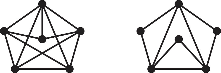
Graphs realizing
It is easily deduced from Theorem 4.3 that if the sets
5 Graphs realizing multisets
S
{
i
,
j
}
n
n
−
1
In this section, we provide a criterion for
Theorem 5.1
If
Proof
Suppose, on the contrary, that
Then, by Theorem 2.5, the Laplacian spectrum of
where the eigenvalues are not in the increasing order.
Since 1 is a simple Laplacian eigenvalue of
On the other hand, the number 2 is also a simple Laplacian eigenvalue of
5.1 Graphs realizing the multisets
S
{
2
,
j
}
n
n
−
1
First, we describe the multisets
Theorem 5.2
Let
If
If
If
If
Proof
For
If
For
The cases (iii) and (iv) can be proved analogously with the use of Lemmas 3.3, 4.2 and 3.4, respectively.□
In the following theorem, we discuss construction of graphs realizing the multisets
Theorem 5.3
Let
Proof
Let
Conversely, if
5.2 Graphs realizing the multisets
S
{
1
,
j
}
n
n
−
1
Now we are in a position to study the realizability of the multisets
Theorem 5.4
Let G be a simple connected graph of order n,
For
For
Proof
(i) If
Suppose first that
Thus, the graph
If
If
Assume now that the graph
Thus, the graph
Let
If
Suppose now that
Thus, we obtained that if
(ii) Let now
As above, we first consider the case
Thus, the graph
If
Let now the order of
Suppose now that a graph
As above, we obtain that
If the order of
Let
From the proof of Theorem 5.4, one can easily see the structure of graphs realizing
Theorem 5.5
Let G be a graph of order
The graph G realizes
The graph G realizes
6
S
{
i
,
n
}
n
m
-conjecture
This section is devoted to describing necessary conditions on the multiset
First, we note that by Theorem 2.6, any graph realizing
Proposition 6.1
If G realizes
Thus, together with
Note that since the equalities
According to the study by Cvetković et al. [5, p. 286–289] and Tables A1–A3 in Appendix A, there are no graphs of order less than 6 realizing
Proposition 6.2
If
Proof
Let
As the number of spanning trees is an integer,
From Lemma 3.3, we obtain another simple observation.
Proposition 6.3
Let n be a positive integer,
As we noted above, graphs realizing
Thus, for
Conjecture 6.4
For
In light of this conjecture, we have the following.
Conjecture 6.5
For
Note that Conjecture 6.5 follows from Conjecture 6.4, the
7 Conclusion
Inspired by the work [9] by Fallat et al. on the sets
There is another approach to study the multisets
Some Laplacian integral graphs that realizing
| Construction | Laplacian spectrum |
|
|---|---|---|
|
|
|
|
|
|
|
|
|
|
|
|
|
|
|
|
|
|
|
|
|
|
|
|
|
|
|
|
|
|
|
|
|
|
|
|
|
|
|
|
|
|
|
|
|
|
|
|
|
|
|
|
Problem 1
Given a multiset
Acknowledgment
The work of M. Tyaglov was partially supported by the National Natural Science Foundation of China under grant no. 11901384.
-
Conflict of interest: The authors state that there is no conflict of interest.
-
Data availability statement: Data sharing is not applicable to this article as no datasets were generated or analysed during the current study.
Appendix A List of Laplacian integral graphs realizing
S
{
i
,
j
}
n
m
up to order 7
From the studies by Cvetković and Petrić [4] and Cvetković et al. [5, p. 286], it follows that there are totally six connected graphs of order 4, 21 connected graphs of order 5, and 112 ones of order 6. In [5, p. 301–304], the authors depicted graphs of the order less than 6 and found their Laplacian spectra. Thus, it is known that there are exactly five Laplacian integral graphs of order 4 and 12 Laplacian graphs of order 5. Cvetković and Petrić [4] depicted all these graphs of order 6 without calculating their Laplacian spectra. In the study by Grone and Merris [12], it was mentioned that there are exactly 37 Laplacian integral graphs. Here, we list all graphs realizing multisets
Below and throughout the text of the article, we use the following notations:
References
[1] M. Anđelić, T. Koledin, and Z. Stanić, Signed graphs whose all Laplacian eigenvalues are main, Linear Multilinear Algebra 71 (2023), 2409–2425. 10.1080/03081087.2022.2105288Suche in Google Scholar
[2] S. Banerjee, Laplacian spectrum of comaximal graph of the ring Zn, Spec. Matrices 10 (2022), 285–298. 10.1515/spma-2022-0163Suche in Google Scholar
[3] H.-Y. Ching, R. Flórez, and A. Mukherjee, Families of integral cographs within a triangular array, Spec. Matrices 8 (2020), 257–273. 10.1515/spma-2020-0116Suche in Google Scholar
[4] D. Cvetković and M. Petrić, A table of connected graphs on six vertices, Discrete Math. 50 (1984), 37–49. 10.1016/0012-365X(84)90033-5Suche in Google Scholar
[5] D. Cvetković, P. Rowlinson, and S. Simić, An introduction to the theory of graph spectra, London Mathematical Society Student Texts, vol. 75, Cambridge University Press, Cambridge, 2010. 10.1017/CBO9780511801518Suche in Google Scholar
[6] D. Cvetković, I. Gutman, and N. Trinajstić, Conjugated molecules having integral graph spectra, Chem. Phys. Lett. 29 (1974), 65–86. 10.1016/0009-2614(74)80135-1Suche in Google Scholar
[7] D. Cvetković and T. Davidović, Multiprocessor interconnection networks with small tightness, Int. J. Found. Comput. Sci. 20 (2009), 941–963. 10.1142/S0129054109006978Suche in Google Scholar
[8] L. S. de Lima, N. M. M. de Abreu, C. S. Oliveira, and M. A. A. de Freitas, Laplacian integral graphs in S(a,b), Linear Algebra Appl. 423 (2007), 136–145. 10.1016/j.laa.2006.12.004Suche in Google Scholar
[9] S. M. Fallat, S. J. Kirkland, J. J. Molitierno, and M. Neumann, On graphs whose Laplacian matrices have distinct integer eigenvalues, J. Graph Theory 50 (2005), 162–174. 10.1002/jgt.20102Suche in Google Scholar
[10] M. Fiedler, Algebraic connectivity of graphs, Czechoslovak Math. J. 23 (1973), 298–305. 10.21136/CMJ.1973.101168Suche in Google Scholar
[11] A. Goldberger and M. Neumann, On a conjecture on a Laplacian matrix with distinct integral spectrum, J. Graph. Theory 72 (2013), 178–208. 10.1002/jgt.21638Suche in Google Scholar
[12] R. Grone and R. Merris, The Laplacian spectrum of a graph. II, SIAM J. Discrete Math. 7 (1994), 221–229. 10.1137/S0895480191222653Suche in Google Scholar
[13] R. Grone and R. Merris, Indecomposable Laplacian integral graphs, Linear Algebra Appl. 428 (2008), 1565–1570. 10.1016/j.laa.2007.09.025Suche in Google Scholar
[14] A. Hameed, Z. U. Khan, and M. Tyaglov, Laplacian energy and first Zagreb index of Laplacian integral graphs, An. Ştiinţ. Univ. “Ovidius” Constanţa Ser. Mat. 30 (2022), 133–160. Suche in Google Scholar
[15] A. Hameed and M. Tyaglov, Integral Laplacian graphs with a unique repeated Laplacian eigenvalue, II, 2022, submitted. ArXiV: 2307.07275. 10.1515/spma-2023-0111Suche in Google Scholar
[16] P. L. Hammer and A. K. Kel’mans, Laplacian spectra and spanning trees of threshold graphs, First Int. Colloquium Graphs Optimiz. (GOI), Grimentz 65 (1996), 255–273. 10.1016/0166-218X(94)00049-JSuche in Google Scholar
[17] F. Harary and A. J. Schwenk, Which graphs have integral spectra? in: Graphs and combinatorics (R. Bari and F. Harary, eds.), Graphs and Combinatorics, Proc. Capital Conf. George Washington University, Washington, D.C., 1973; Lecture Notes in Mathematics, Springer-Verlag, Berlin, 406 (1974), 45–51. 10.1007/BFb0066434Suche in Google Scholar
[18] A. K. Kel’mans, The number of trees in a graph. I, Avtomat. i Telemekh 26 (1965), 2194–2204. Suche in Google Scholar
[19] S. Kirkland, Completion of Laplacian integral graphs via edge addition, Discrete Math. 295 (2005), 75–90. 10.1016/j.disc.2004.12.010Suche in Google Scholar
[20] S. Kirkland, Constructably Laplacian integral graphs, Linear Algebra Appl. 423 (2007), 3–21. 10.1016/j.laa.2006.07.012Suche in Google Scholar
[21] S. Kirkland, Laplacian integral graphs with maximum degree 3, Electron. J. Combin. 15 (2008), 120. 10.37236/844Suche in Google Scholar
[22] R. Merris, Degree maximal graphs are Laplacian integral, Linear Algebra Appl. 199 (1994), 381–389. 10.1016/0024-3795(94)90361-1Suche in Google Scholar
[23] R. Merris, Laplacian matrices of graphs: a survey, Linear Algebra Appl. 197/198 (1994), 143–176.10.1016/0024-3795(94)90486-3Suche in Google Scholar
[24] R. Merris, Large families of Laplacian isospectral graphs, Linear Multilinear Algebra 43 (1997), 201–205. 10.1080/03081089708818525Suche in Google Scholar
[25] R. Merris, Threshold graphs, In: Proceedings of the Prague Mathematical Conference 1996, Icaris, Prague, 1997, pp. 205–210. Suche in Google Scholar
[26] R. Merris, Laplacian graph eigenvectors, Linear Algebra Appl. 278 (1998), 221–236. 10.1016/S0024-3795(97)10080-5Suche in Google Scholar
[27] J. J. Molitierno, Applications of combinatorial matrix theory to Laplacian matrices of graphs, Discrete Mathematics and its Applications, CRC Press, Boca Raton, FL, 2012. Suche in Google Scholar
[28] J. Sander and T. Sander, Recent developments on the edge between number theory and graph theory, From Arithmetic to Zeta-Functions: Number Theory in Memory of Wolfgang Schwarz, 2016, pp. 405–425. 10.1007/978-3-319-28203-9_24Suche in Google Scholar
[29] Z. Stanić, Laplacian controllability for graphs with integral Laplacian spectrum, Mediter. J. Math. 18 (2021), 35. 10.1007/s00009-020-01684-3Suche in Google Scholar
© 2023 the author(s), published by De Gruyter
This work is licensed under the Creative Commons Attribution 4.0 International License.
Artikel in diesem Heft
- Research Articles
- Determinants of some Hessenberg matrices with generating functions
- On monotone Markov chains and properties of monotone matrix roots
- On the spectral properties of real antitridiagonal Hankel matrices
- The complete positivity of symmetric tridiagonal and pentadiagonal matrices
- Two n × n G-classes of matrices having finite intersection
- On new universal realizability criteria
- On inverse sum indeg energy of graphs
- Incidence matrices and line graphs of mixed graphs
- Diagonal dominance and invertibility of matrices
- New versions of refinements and reverses of Young-type inequalities with the Kantorovich constant
- W-MPD–N-DMP-solutions of constrained quaternion matrix equations
- Representing the Stirling polynomials σn(x) in dependence of n and an application to polynomial zero identities
- The effect of removing a 2-downer edge or a cut 2-downer edge triangle for an eigenvalue
- Idempotent operator and its applications in Schur complements on Hilbert C*-module
- On the distance energy of k-uniform hypergraphs
- The bipartite Laplacian matrix of a nonsingular tree
- Combined matrix of diagonally equipotent matrices
- Walks and eigenvalues of signed graphs
- On 3-by-3 row stochastic matrices
- Legendre pairs of lengths ℓ ≡ 0 (mod 5)
- Integral Laplacian graphs with a unique repeated Laplacian eigenvalue, I
- Communication
- Class of finite-dimensional matrices with diagonals that majorize their spectrum
- Corrigendum
- Corrigendum to “Spectra universally realizable by doubly stochastic matrices”