The bipartite Laplacian matrix of a nonsingular tree

Ravindra B. Bapat; Rakesh Jana; Sukanta Pati

doi:10.1515/spma-2023-0102

Artikel Open Access

The bipartite Laplacian matrix of a nonsingular tree

Ravindra B. Bapat , Rakesh Jana und Sukanta Pati

Veröffentlicht/Copyright: 27. August 2023

Veröffentlicht von

Veröffentlichen auch Sie bei De Gruyter Brill

Manuskript einreichen Informationen für Autor*innen Erkunden Sie dieses Fachgebiet

Aus der Zeitschrift Special Matrices Band 11 Heft 1

Abstract

For a bipartite graph, the complete adjacency matrix is not necessary to display its adjacency information. In 1985, Godsil used a smaller size matrix to represent this, known as the bipartite adjacency matrix. Recently, the bipartite distance matrix of a tree with perfect matching was introduced as a concept similar to the bipartite adjacency matrix. It has been observed that these matrices are nonsingular, and a combinatorial formula for their determinants has been derived. In this article, we provide a combinatorial description of the inverse of the bipartite distance matrix and establish identities similar to some well-known identities. The study leads us to an unexpected generalization of the usual Laplacian matrix of a tree. This generalized Laplacian matrix, which we call the bipartite Laplacian matrix, is usually not symmetric, but it shares many properties with the usual Laplacian matrix. In addition, we study some of the fundamental properties of the bipartite Laplacian matrix and compare them with those of the usual Laplacian matrix.

Keywords: tree; distance matrix; Laplacian matrix; bipartite distance matrix; bipartite Laplacian matrix

MSC 2010: 05C05; 05C12; 05C50; 15A15

1 Introduction

Let G be an undirected, simple, connected graph with vertex set V = { 1 , 2 , … , n } and edge set E . We use u ∼ v to mean that the vertices u and v are adjacent. The symbol [ u , v ] means the edge between u and v . The degree of a vertex v is denoted by d G ( v ) or simply by d ( v ) . The distance between two vertices u and v is denoted by dist G ( u , v ) or simply by dist ( u , v ) .

The adjacency matrix A ( G ) = [ a i j ] of G is a square matrix with a i j = 1 if i ∼ j and 0 otherwise. The square matrix D ( G ) ≔ [ dist ( i , j ) ] is called the distance matrix of G . The usual Laplacian matrix ℒ ( G ) is a square matrix such that ( i , j ) th entry is − a i j if i ≠ j and d ( i ) if i = j . For an m × n matrix M and subsets X of { 1 , … , m } and Y ⊆ { 1 , … , n } , the notation M ( X ∣ Y ) denotes the submatrix of M obtained by excluding the rows indexed by X and the columns indexed by Y . M ( X , Y ) denotes the submatrix of M determined by the rows corresponding to X and columns corresponding to Y .

We generally follow the terminology used in the study by Cvetkovic et al. [11]. The distance matrix has several applications in many different areas like telecommunication, molecular stability, graph embedding theory, and network flow algorithms and has been a subject of various independent studies. In [16], Graham and Pollak established a correlation between the addressing problem in data communication systems and the number of negative eigenvalues in the distance matrix. In the same study [16], it was shown that if T is a tree with n vertices, then the determinant of the distance matrix D ( T ) is ( − 1 ) n − 1 2 n − 2 ( n − 1 ) , which is independent of the structure of T and depends only on the number of vertices of T . Subsequently, Graham et al. [14] in 1977 showed that the determinant det D ( G ) of a graph G depends only on the blocks of G and not on how they are assembled. A formula for the inverse of the distance matrix of a tree was given by Graham and Lovász [15]. The distance matrix generated considerable interest and a plethora of extensions and generalizations have been proved (see, e.g., [2,5–9,19,23,24]).

Let G be a labeled, connected, bipartite graph with the vertex bipartition ( L = { l 1 , … , l m } , R = { r 1 , … , r n } ) . For a bipartite graph, we do not require the complete adjacency matrix to display the adjacency information in the graph. Godsil [13] in 1985, used a smaller size matrix to display this information. Later on, this matrix was named the bipartite adjacency matrix, see [10,22]. The bipartite adjacency matrix A of G is the m × n submatrix of its adjacency matrix determined by the rows corresponding to L and the columns corresponding to R . We refer interested readers to [10,13,22] for knowing more about the bipartite adjacency matrix.

In a recent article [4], we have introduced the bipartite distance matrix of a bipartite graph G with a unique perfect matching and observed that the bipartite distance matrix of a tree T with a unique perfect matching is deeply related to the structure of the tree T and many interesting combinatorial properties were supplied. In this article, we shall show how the study of that matrix naturally leads us to a surprising nontrivial generalization of the usual Laplacian matrix.

Let us define the bipartite distance matrix. Let G be a labeled, connected, bipartite graph with the vertex bipartition ( L = { l 1 , … , l p } , R = { r 1 , … , r p } ) . Then, we call D ( L , R ) the bipartite distance matrix and denote it by B G or simply B . This is the submatrix of the distance matrix D of G determined by the rows corresponding to L and columns corresponding to R . If G has a unique perfect matching ℳ , we can use it to define a “canonical” way to order L ≔ { l 1 , … , l p } and R ≔ { r 1 , … , r p } such that [ l 1 , r 1 ] , … , [ l p , r p ] are matching edges of G . We call such a bipartition, a standard vertex bipartition of G . So, the ( i , j ) th entry of B is the distance dist ( l i , r j ) in G .

If G is a bipartite graph with a unique perfect matching, then we can have many standard vertex bipartitions. However, we can see that the bipartite distance matrices corresponding to them are similar to each other.

A tree T is called a nonsingular tree if the adjacency matrix A ( T ) of T in invertible. It is well known that T is nonsingular if and only if it has a unique perfect matching. As a tree is a bipartite graph, the study of the properties of a bipartite distance matrix of a nonsingular tree is naturally a starting point.

Recall that the determinant formula of Graham and Pollack for a tree T on n vertices establishes that det D ( T ) is always a multiple of 2 n − 2 . Quite similar to that, it was shown in [4,18] that for a nonsingular tree T on n = 2 p vertices, the number det B ( T ) is a multiple of 2 p − 1 . Interestingly, it turns out that this is the highest power of 2 that can divide det B ( T ) . So, the factor bd ( T ) ≔ det B ( T ) ∕ ( − 2 ) p − 1 is called the bipartite distance index of T becomes an interesting object to study.

It turns out that this number is closely related to the combinatorial properties of the given tree. A complete characterization of bd ( T ) was supplied using the structure of T and is described as follows.

An alternating path in a nonsingular tree T is a path with the starting edge, each alternate edge thereafter, and the last edge from the matching (so, the remaining edges are nonmatching edges). By [ u , … , v ] , we mean the unique u - v path in the tree T . By A T , we mean the set of all alternating paths in T (a path [ u , … , v ] is treated to be the same as [ v , … , u ] ).

Theorem 1

[4, 18] Let T be a nonsingular tree on 2 p vertices and S = ( 1 , 1 , 3 , 3 , … ) be a sequence. Then, for any standard vertex bipartition,

bd ( T ) = ∑ P ∈ A T P = [ u , … , v ] [ d ( u ) − 2 ] [ d ( v ) − 2 ] S ∣ P ∣ 2 .

We have noted that the bipartite distance matrix of a nonsingular tree is always invertible, and its determinant can be described using the structure of T . What about the inverse? Can the entries of the inverse be described combinatorially? For the usual distance matrix, such a description can be found in the work of Graham and Lovasz [15].

Even more interestingly, recall that the inverse of the usual distance matrix has a definite relationship with the Laplacian matrix.

Theorem 2

[5] Let T be a tree on n vertices. For each i = 1 , … , n , let δ i = 2 − d ( i ) and put δ t = [ δ 1 , … , δ n ] . Then,

D ( T ) − 1 = − 1 2 ℒ ( T ) + 1 2 ( n − 1 ) δ δ t .

Can we have a similar statement for the bipartite distance matrix too? In that case, what is an appropriate replacement for the Laplacian matrix? We call it the bipartite Laplacian matrix. With the help of the bipartite Laplacian matrix, we provide a formula for the inverse of the bipartite distance matrix in Theorem 24. It turns out that the usual Laplacian matrix of any tree is a very special case of the bipartite Laplacian matrix, and this matrix has many properties similar to those of a Laplacian, see Theorem 9. We supply that definition below.

An alternating path is called an odd alternating path if it has an odd number of matching edges, and an alternating path is called an even alternating path if it has an even number of matching edges.

Definition

Let T be a nonsingular tree T on 2 p vertices and ( L , R ) be a standard vertex bipartition of T . The bipartite Laplacian matrix of T , denoted by L ( T ) or simply by L , is the p × p matrix whose rows are indexed by r 1 , … , r p and the columns are indexed by l 1 , … , l p . The ( i , j ) th entry of L ( T ) , denoted by L i j , is defined as follows:

L i j = d ( r i ) d ( l i ) − 1 if i = j ; d ( r i ) d ( l j ) if i ≠ j and the r i – l j path is an odd alternating path ; − d ( r i ) d ( l j ) if i ≠ j and the r i – l j path is an even alternating path ; − 1 if i ≠ j and r i ∼ l j ; 0 otherwise .

Remark 3

Here, we want to emphasize that in the definition of bipartite distance matrix of a nonsingular tree T , we indexed rows by l 1 , … , l p and columns by r 1 , … , r p . But, in the definition of bipartite Laplacian matrix, we indexed rows by r 1 , … , r p and columns by l 1 , … , l p .

Let us first look at an example.

Example 4

Consider the nonsingular tree T as shown below.

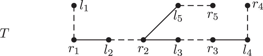
Here, the dashed edges are the matching edges. Clearly, L = { l 1 , … , l 5 } and R = { r 1 , … , r 5 } is the standard vertex bipartition. The bipartite distance matrix B and the bipartite Laplacian matrix L are

B = 1 3 5 7 5 1 1 3 5 3 3 1 1 3 3 5 3 1 1 5 3 1 3 5 1 L = 1 − 1 0 0 0 − 3 5 − 1 0 − 1 2 − 4 3 − 1 0 − 1 2 − 2 1 0 1 − 2 0 0 1 .

We now supply some motivation to study the bipartite Laplacian matrix. Let T be any tree. Denote by T ′ the nonsingular tree obtained by adding a new pendant vertex at every vertex of T . This T ′ is usually called a corona. We denote it by T ∘ K 1 . It can be easily seen that the bipartite Laplacian L ( T ′ ) of T ′ is nothing but the Laplacian ℒ ( T ) of T . Note that the bipartite Laplacian is usually not symmetric. However, it still has many properties like the Laplacian. Therefore, to understand the usual Laplacian matrix of tree in a bigger picture, one needs to study the bipartite Laplacian matrix. Another motivation to study this matrix is that even though its size is half the number of vertices (of the nonsingular tree), it still gives us some information about the tree. It may save us some time.

We want to emphasize that there are many generalizations of the usual Laplacian matrix ℒ of a graph G that have been studied in the literature. For example, the q -Laplacian matrix [6], the distance Laplacian matrix [1], the normalized Laplacian matrix, and the normalized distance Laplacian matrix [21]. Each of these generalizations involves obtaining the usual Laplacian matrix by substituting a particular value (e.g., q = 1 ) or viewing the generalized version as the usual Laplacian matrix of the same graph but with some assigned edge weights. On the other hand, the bipartite Laplacian matrix is a different kind of generalization of the usual Laplacian matrix. To obtain the usual Laplacian matrix of a tree F (not necessarily a nonsingular tree), we have to find the bipartite Laplacian matrix of some nonsingular tree T , which may not necessarily be the same as F . This aspect makes the study of the bipartite Laplacian matrix even more interesting.

The document is organized as follows. In Section 2, we first relate the structure of the bipartite Laplacian matrix of a new tree with that of the old one using signed degree vector. Using this, we study some of the fundamental properties of the bipartite Laplacian matrix and compare them with those of the usual Laplacian matrix. Furthermore, we discuss how a multiplicity of an eigenvalue of the bipartite Laplacian matrix of a nonsingular tree is related to the tree structure. In Section 3, we present a formula for the inverse of the bipartite distance matrix of a nonsingular tree using its bipartite Laplacian matrix. Using this, we obtain a lower bound on the geometric multiplicity of the eigenvalue − 2 of the bipartite distance matrix of a nonsingular tree.

2 The bipartite Laplacian matrix

In this section, we shall examine some of the fundamental properties of the bipartite Laplacian matrix and discuss how a multiplicity of an eigenvalue of the bipartite Laplacian matrix of a nonsingular tree is related to the tree structure. For our purposes, all vectors are column vectors, and we shall use transpose to talk about row vectors. We use the notation 1 to denote the vector of all ones of an appropriate size. Additionally, we use e k to denote a vector of an appropriate size where all entries are zero except for the k th entry, which is set to 1.

Let us start the discussion with the following observation.

Remark 5

Let T be a nonsingular tree on 2 p vertices with a standard vertex bipartition ( L , R ) .

Let F be the tree obtained by interchanging the labels of l i with r i for all i = 1 , … , p in T . Then, L ( T ) = L ( F ) t , and both are similar.
Let F be the tree obtained by relabeling the vertices within the part L , keeping it a standard vertex bipartition (i.e., we also relabel the respective vertices in R accordingly). Then, L ( T ) is permutation similar to L ( F ) .

Definition

Let T be a tree and v be a vertex. Let T ^ be the tree obtained from T by introducing two new vertices u and w and adding the edges [ v , u ] and [ u , w ] . We refer to this operation as attaching a new P 2 at the vertex v.
Let T be a nonsingular tree on 2 p vertices with the standard vertex bipartition ( L , R ) . Let T ^ be the tree obtained by attaching a new P 2 at some vertex v ∈ T . To compute its bipartite Laplacian matrix, we need to label the new vertices. We adopt the following procedure for that:
1. if v ∈ L , then we put u = r p + 1 , w = l p + 1 , and
2. if v ∈ R , then we put u = l p + 1 , w = r p + 1 .

We now introduce the concept of a signed degree vector at a vertex, which is required to relate the structure of the bipartite Laplacian of the new tree with that of the old one.

Definition

Let T be a nonsingular tree on 2 p vertices with the standard vertex bipartition ( L , R ) and v be a vertex. Then, the signed degree vector μ v at v is defined as follows:

If v ∈ L , then for i = 1 , … , p , we define
1. μ v ( i ) = d T ( r i ) if the v – r i path is an odd alternating path,
2. μ v ( i ) = − d T ( r i ) if the v – r i path is an even alternating path, and
3. μ v ( i ) = 0 if the v – r i path is not an alternating path.
In a similar way, if v ∈ R , then for i = 1 , … , p , we define
1. μ v ( i ) = d T ( l i ) if the v – l i path is an odd alternating path,
2. μ v ( i ) = − d T ( l i ) if the v – l i path is an even alternating path, and
3. μ v ( i ) = 0 if the v – l i path is not an alternating path.

Thus, for the tree T in Example 4, we have

μ l 2 = 0 3 − 2 1 − 1 t and μ r 3 = 1 − 2 2 0 0 t .

In the following result, we relate the structure of the bipartite Laplacian L of the new tree with that of the old one.

Lemma 6

Let T be a nonsingular tree on 2 p vertices with a standard vertex bipartition ( L , R ) . Let T ^ be the tree obtained from T by attaching a new P 2 at v . Let μ v be the signed degree vector at v of T .

If v = l k for some k , then L ( T ^ ) = L ( T ) + μ v e k t − μ v − e k t 1 .
If v = r k for some k , then L ( T ^ ) = L ( T ) + e k μ v t − e k − μ v t 1 .

Proof

We only provide the proof of item (a) as the proof of item (b) can be dealt in a similar way. Without loss of any generality, let us assume that T ^ be obtained from T by adding a new path [ l k , r p + 1 , l p + 1 ] for some 1 ≤ k ≤ p . Clearly, L ^ = L ∪ { l p + 1 } and R ^ = R ∪ { r p + 1 } is a standard vertex bipartition of T ^ . Let L and L ^ be the bipartite Laplacian matrix of T and T ^ , respectively. Since [ r p + 1 , l p + 1 ] is the only alternating path that starts at r p + 1 and d T ^ ( r p + 1 ) = 2 with [ r p + 1 , l k ] is not a matching edge, it follows that all entries of ( p + 1 ) th row of L ^ is zero except L ^ ( p + 1 , p + 1 ) = d T ^ ( r p + 1 ) d T ^ ( l p + 1 ) − 1 = 1 and L ^ ( p + 1 , k ) = − 1 . Hence, L ^ ( p + 1 , : ) = − e k t 1 .

Let us take i = 1 , … , p . Then, r i ≁ l p + 1 . Note that the l k – r i path is an odd alternating path if and only if the l p + 1 – r i path is an even alternating path. Similarly, the l k – r i path is an even alternating path if and only if the l p + 1 – r i path is an odd alternating path. Since d T ^ ( l p + 1 ) = 1 , it follows that L ^ ( { 1 , … , p } , p + 1 ) = − μ l k , where μ l k is the signed degree vector of T at l k .

Since d T ( u ) = d T ^ ( u ) for each u ∈ T other than l k , it follows that L ^ ( i , j ) = L ( i , j ) for each i = 1 , … , p and j = 1 , … , k − 1 , k + 1 , … , p .

Finally, we note that d T ^ ( l k ) = d T ( l k ) + 1 . Therefore, for i = 1 , … , p , we have

L ^ ( i , k ) = d T ( r i ) ( d T ( l k ) + 1 ) − 1 if i = k ; d T ( r i ) ( d T ( l k ) + 1 ) if i ≠ k and the r i – l k path is an odd alternating path ; − d T ( r i ) ( d T ( l k ) + 1 ) if i ≠ k and the r i – l k path is an even alternating path ; − 1 if i ≠ k and r i ∼ l k ; 0 otherwise .

Therefore, L ^ ( { 1 , … , p } , k ) = L ( { 1 , … , p } , k ) + μ l k . This completes the proof.□

The signed degree vector at a vertex v has the property that the sum of its entries is always one.

Lemma 7

Let T be a nonsingular tree on 2 p vertices with a standard bipartition ( L , R ) . Let u be any vertex in T and μ u be the signed degree vector at u. Then, 1 t μ u = 1 .

Proof

We proceed by induction on p ≥ 1 . For p = 1 , the result is trivial. Assume the result to be true for nonsingular trees with less than 2 p vertices. Let T be a nonsingular tree on 2 p vertices with a standard bipartition ( L , R ) . Let u ∈ R . (The case of u ∈ L can be dealt similarly.) Let μ be the signed degree vector of u in T .

Suppose [ v 0 , v 1 , … , v k ] is a longest path in T . As p > 1 , we have k ≥ 3 and so we may assume that v 0 , v 1 ≠ u . As T is nonsingular and this is a longest path, we have d ( v 0 ) = 1 and d ( v 1 ) = 2 . Without loss of any generality, let us assume v 0 , v 1 ∈ { l p , r p } . Let T ^ = T − { v 0 , v 1 } be the tree obtained from T by removing the vertices v 0 and v 1 . Clearly, u ∈ T ^ . Let μ ^ be the signed degree vector of u in T ^ . Note that μ ^ is vector of size p − 1 . Clearly, d T ( v ) = d T ^ ( v ) for each v ∈ T ^ − v 2 and d T ( v 2 ) = d T ^ ( v 2 ) + 1 . It follows that μ ( i ) = μ ^ ( i ) for each l i ∈ L \ { v 2 } .

If either v 2 ∈ R or the u – v 2 path is not an alternating path, then μ = μ ^ 0 and the result follows by induction. Now we assume that v 2 ∈ L and the u – v 2 path is an alternating path. Then, v 2 ∼ r p and d T ( l p ) = 1 . Let v 2 = l k for some 1 ≤ k < p . Note that the u – l p path is also an alternating path and so we have μ ^ ( k ) = ( − 1 ) t d T ^ ( v 2 ) for some t and μ ( p ) = ( − 1 ) t + 1 . Since μ ( k ) = ( − 1 ) t d T ( v 2 ) = μ ^ ( k ) + ( − 1 ) t , it follows that

μ = μ ^ t ( − 1 ) t + 1 t + ( − 1 ) t e k 0 t .

Hence, the result follows by induction.□

We now recall a well-known result. It can be found, e.g., in [3, Lemma 4.2].

Lemma 8

Let M be a square matrix of order n with zero row and column sums. Then, the cofactors of any two elements of M are equal.

Below, we have provided some elementary properties of the bipartite Laplacian matrix and compare them with those of the usual Laplacian matrix, whenever possible.

Theorem 9

Let T be a nonsingular tree on 2 p vertices with a standard vertex bipartition ( L , R ) . Suppose L is the bipartite Laplacian matrix of T. Then, the following assertions hold.

The row and column sums of L are zero. (A similar property also holds for the usual Laplacian matrix of any graph.)
The cofactors of any two elements of L are equal to 1. (For the usual Laplacian matrix of a graph, the cofactors of any two elements are equal to the number of spanning trees.)
The rank of L is n − 1 . (A similar result is also true for the usual Laplacian matrix of a connected graph.)
The algebraic multiplicity of 0 as an eigenvalue of L is 1. (A similar result is also true for the usual Laplacian matrix of a connected graph.)
If u is an eigenvector of L corresponding to an eigenvalue λ ≠ 0 , then 1 t u = 0 . (A similar property also holds for the usual Laplacian matrix of any graph.)
If T = F ∘ K 1 for some tree F on p vertices, then ℒ ( F ) = L ( T ) , where ℒ is the usual Laplacian matrix of F. (That is, the usual Laplacian matrix of a tree F can be seen as a bipartite Laplacian matrix of another tree T.)
The matrix L is a symmetric matrix if and only if T is a corona tree, i.e., if T = F ∘ K 1 for some tree F. (However, the usual Laplacian matrix is always a symmetric matrix.)

Proof of Item (a). The result follows from Lemmas 6 and 7.

Proof of Item (b). By Lemma 8, all cofactors of L are equal. We only need to show that they are equals to 1. We proceed by induction on p ≥ 2 . The statement is valid for p = 2 . Assume it holds for all nonsingular trees with vertices less than 2 p . Let T be a nonsingular tree with 2 p vertices. Without loss of any generality, we assume that l p is a pendant vertex in T and d ( r p ) = 2 . Let r p be adjacent to l k , for some 1 ≤ k < p . Let T ′ be the tree obtained from T by deleting vertices l p and r p from T . Let L ′ be the bipartite Laplacian matrix of T ′ . Consider a vertex r i such that 1 ≤ i < p . By Lemma 6, it follows that

det L ( i ∣ p ) = ( − 1 ) p + k L ′ ( i ∣ k ) = ( − 1 ) i + p .

The last identity follows by induction hypothesis. Hence, the result follows.

Proof of Item (c). By item (a), 0 is an eigenvalue of L . The remaining part of the proof follows from item (b).

Proof of Item (d). By item (a), the characteristic polynomial χ ( x ) ≔ det ( x I − L ( T ) ) = x f ( x ) , where f ( x ) is some polynomial with integer coefficients. By item (b), it follows that

f ( 0 ) = coefficient of x in χ ( x ) = ( − 1 ) p − 1 × ( sum of the principal minors of L of size p − 1 ) = ( − 1 ) p − 1 p .

This shows that the algebraic multiplicity of 0 is 1.

Proof of Item (e). It directly follows from the fact that 1 t L = 0 .

Proof of Item (f). Let us assume that T = F ∘ K 1 for some tree F on p vertices. Note that, for each v ∈ F , we have d T ( v ) > 1 , and there exists a leaf u ∉ F adjacent to v in T . Therefore, for each i = 1 , … , p , exactly one of l i and r i is in F . We label the vertex v ∈ F by v i if v is adjacent to a pendant vertex l i or r i in T . Now note that the ( i , i ) th entry of L is d T ( l i ) d T ( r i ) − 1 = d T ( v i ) − 1 = d F ( v i ) .

Now consider i ≠ j . Since each edge in F is a nonmatching edge in T , all v i – v j paths in T are not an alternating path in T . Therefore, if v i ≁ v j , then both the r i – l j path and the r j – l i path are not an alternating path and so L ( i , j ) = L ( j , i ) = 0 . Suppose v i ∼ v j . Without loss of any generality, let us assume v i = l i , then v j = r j . It follows that the r i – l j path is an alternating path of length 3 and r j ∼ l i . Therefore, L ( i , j ) = − d T ( r i ) d T ( l j ) = − 1 and L ( j , i ) = − 1 . This shows that L = ℒ .

Proof of Item (g). Let T not be a corona tree. Then, there exists an alternating path P = [ v 0 , v 1 , v 2 , v 3 ] such that d ( v 0 ) = 1 , d ( v 3 ) > 1 . By taking v 0 = l 1 and v 2 = l 2 , we see that the ( 1 , 2 ) th entry of L is − 1 but ( 2 , 1 ) th entry of L is − d ( v 3 ) ≠ − 1 . This completes the proof.

By item (f) of Theorem 9, all eigenvalues of the bipartite Laplacian matrix of a corona tree are nonnegative real numbers. An interesting question now arises: Can it be true that all eigenvalues of the bipartite Laplacian of each nonsingular tree are nonnegative real numbers? Let us investigate it for the tree T as in Example 4. Let L be the bipartite Laplacian matrix of the tree T as in Example 4. Let f ( x ) = det ( x I − L ) be the characteristic polynomial of L . By a direct computation, we see that f ( x ) = x ( x 4 − 11 x 3 + 31 x 2 − 24 x + 5 ) . Clearly, 0 is an eigenvalue of L . We can further observe that f ( 1 ∕ 4 ) > 0 , f ( 1 ∕ 2 ) < 0 , f ( 1 ) > 0 , f ( 3 ) < 0 , and f ( 10 ) > 0 . Therefore, all eigenvalues of L are nonnegative real numbers, whereas L is not a symmetric matrix, which is quite interesting and seems to be true for the bipartite Laplacian matrix of each nonsingular tree.

Theorem 10

(Conjecture) Let T be a nonsingular tree on 2 p vertices with a standard vertex bipartition ( L , R ) . Then, all eigenvalues of the bipartite Laplacian matrix are nonnegative real numbers.

From item (b) of Theorem 9, we note that all cofactors of the bipartite Laplacian matrix of a nonsingular tree T is 1. At this point, we also have a description of all minors of the bipartite Laplacian matrix of a nonsingular tree. However, the discussion would require some more combinatorial developments, hence we postpone it.

Recall that, for the usual Laplacian matrix, bounds on the multiplicity 1 as an eigenvalue are well known. Let G be a graph and ℒ ( G ) be its usual Laplacian matrix. p ( G ) and q ( G ) denote the number of pendant vertices and the number of quasipendant vertices of G , respectively. Faria [12] in 1985 observed that the multiplicity of 1 as an eigenvalue of ℒ ( G ) is at least p ( G ) − q ( G ) . (This number was called the star degree of a graph G .) In 1990, Grone et al. [17] gave an upper bound on the multiplicity of any eigenvalue of the usual Laplacian matrix of a tree.

Theorem 11

[17, Theorem 2.3] Let T be a tree on n ≥ 2 vertices and ℒ ( T ) be the usual Laplacian matrix of T. Then, the multiplicity of any eigenvalue of ℒ ( T ) is at most p ( T ) − 1 .

Interestingly, such bounds can also be provided for the bipartite Laplacian matrix of a nonsingular tree. In order to describe that, we need some more terminologies.

Definition

Let T be a nonsingular tree. By a pendant-two-path at w , we mean a path [ u , v , w ] in T such that d T ( u ) = 1 and d T ( v ) = 2 . (As T is nonsingular, it follows that d T ( w ) > 1 .) If [ u , v , w ] is a pendant-two-path at w , then the vertex w is referred as the root of that pendant-two-path.

Let P ( T ) denote the total number of pendant-two-paths (at all vertices) in T . Let Q ( T ) denote the total number of vertices that are root of at least one pendant-two-paths.

Below, we supply a result similar to the previously mentioned Faria’s result for the bipartite Laplacian matrix of a nonsingular tree. Note that we do not yet know whether the bipartite Laplacian matrix is diagonalizable or not.

Theorem 12

Let T be a nonsingular tree on 2 p vertices with a standard vertex bipartition ( L , R ) and L be the bipartite Laplacian matrix of T. Then, the geometric multiplicity of 1 as an eigenvalue of L is at least P ( T ) − Q ( T ) , where P ( T ) and Q ( T ) are defined above.

Proof

Note that if P ( T ) = 0 , then the result holds trivially. So, we assume that P ( T ) ≥ 1 . (Indeed, for any nonsingular tree T , P ( T ) ≥ 2 .) Let w be a vertex in T at which the available pendant-two-paths are [ u i , v i , w ] , i = 1 , … , k . If k = 1 , then the contribution of w to P ( T ) − Q ( T ) is 0. So assume that k > 1 .

Let T ¯ be the tree obtained from T by removing the vertices u 1 , v 1 , … , u k , v k . For i = 1 , … , k , let T i be the tree obtained from T by removing just the two vertices u i and v i from T . Let μ i be the signed degree vector at v of T i , and let μ be the signed degree vector at v of T ¯ . Without loss of any generality, let us assume that the vertex set of T ¯ is { l 1 , … , l n , r 1 , … , r n } . Note that μ i = μ 0 ⋯ 0 t for each i = 1 , … , k , as the edges joining w and any of u 1 , v 1 , … , u k , v k are nonmatching.

Note that for 1 ≤ i ≤ k , u i , z i ∈ { r j i , l j i } for some j i > n . By Lemma 6, we have L = ∗ − μ 1 t ∗ I if w ∈ L and L = ∗ − e q 1 t ∗ I if w ∈ R , where I is an identity matrix and 1 ≤ q ≤ n . It follows that L ( e j i − e j t ) = e j i − e j t for 1 ≤ i < t ≤ k . This completes the proof.□

Next, we supply an upper bound on the geometric multiplicity of an eigenvalue of the bipartite Laplacian matrix of a nonsingular tree. The proof is similar that of Theorem 11 given in [17].

Theorem 13

Let T be a nonsingular tree on 2 p vertices, p > 1 , with a standard vertex bipartition ( L , R ) . Let L be the bipartite Laplacian matrix of T, and let λ be an eigenvalue of L . Then, the geometric multiplicity of λ is at most P ( T ) − 1 .

Proof

We first prove the result for P ( T ) = 2 . Let us assume P ( T ) = 2 . Then, T is a path. Let T = [ r 1 , l 1 , … , r p , l p ] be the path on 2 p vertices. Let L ( T ) be the bipartite Laplacian matrix of T . Let L ( T ¯ ) be the bipartite Laplacian matrix of T ¯ = [ r 1 , l 1 , … , r p − 1 , l p − 1 ] . We claim that if x is an eigenvector of L ( T ) corresponding to an eigenvalue λ ≠ 0 , then x ( p ) ≠ 0 . In order to prove the claim, suppose λ ≠ 0 is an eigenvalue of the bipartite Laplacian matrix of T with a corresponding eigenvector x . Let x ¯ be obtained from x by deleting the p th entry. From L ( T ) x = λ x , by Lemma 6, note that

L ( T ¯ ) x ¯ + μ ( x ( p − 1 ) − x ( p ) ) = λ x ¯ , and − x ( p − 1 ) + x ( p ) = λ x p ,

where μ is a signed degree vector at l p − 1 of T ¯ . If possible let, x p = 0 . Then, x ( p − 1 ) = 0 and L ( T ¯ ) x ¯ = λ x ¯ . Therefore, x ¯ is an eigenvector of T ¯ corresponding to the eigenvalue λ with x ( p − 1 ) = 0 . With a repeated argument, we see that x = 0 , which is a contradiction as x is an eigenvector. Therefore, x ( p ) ≠ 0 .

Suppose that the geometric multiplicity of λ is at least 2. Let x 1 and x 2 be the two linearly independent eigenvectors of L ( T ) corresponding to λ . Then, by a linear combination of x 1 and x 2 , we may find x such that x ( p ) = 0 , which is a contradiction. This shows that if P ( T ) = 2 , then the geometric of λ is 1.

Now suppose P ( T ) = k > 2 and l p − k + 1 , r p − k + 1 , … , l p , r p are the vertices corresponding to these k pendant-two-paths (excluding their roots). Since T is not a path, in view of Remark 5, by relabeling the vertices if necessary, we may assume that d ( l p ) = d ( l p − 1 ) = 1 .

Let x be an eigenvector for λ . We shall show that among x ( p − k + 1 ) , … , x ( p ) , at least two coordinates must be nonzero. If both x ( p ) and x ( p − 1 ) are nonzero, then there is nothing to prove. If possible, let x ( p ) = 0 . Let T ¯ be obtained from T by removing the vertices r p and l p . Let x ¯ be obtained from x by deleting the p th entry.

Note that d ( l p ) = 1 . Let l q , q ≤ p − k , be the root of the pendant-two-path [ l q , r p , l p ] . Then, by item (a) of Lemma 6, in regard to the last row of L , we see that x ( q ) = 0 . It follows that L ( T ¯ ) has λ as an eigenvalue with x ¯ as an eigenvector. Therefore, by using induction it follows that among the coordinates x ( p − k + 1 ) , … , x ( p − 1 ) , there exist at least two coordinates which are nonzero. This establishes that if x is an eigenvector of L , then among x ( p − k + 1 ) , … , x ( p ) , at least two coordinates must be nonzero.

If possible, let x 1 , … , x k be linearly independent eigenvectors of L corresponding to λ . Since for each i = 1 , … , k , among the last k coordinates of x i , at least two coordinates must be nonzero, it follows that by taking an appropriate linear combinations of the vectors x 1 , … , x k , it would be possible to create an eigenvector z such that at most one coordinate among last k coordinates of z is nonzero. Thus, we arrived at a contradiction. Hence, the geometric multiplicity of λ is at most P ( T ) − 1 .□

We remark here that the above two results applied to corona trees provide us the respective known results for the usual Laplacian matrix, as special cases.

In the following result, we discuss how the bipartite Laplacian matrix of a nonsingular tree can be obtained from some of its nonsingular subtrees.

Remark 14

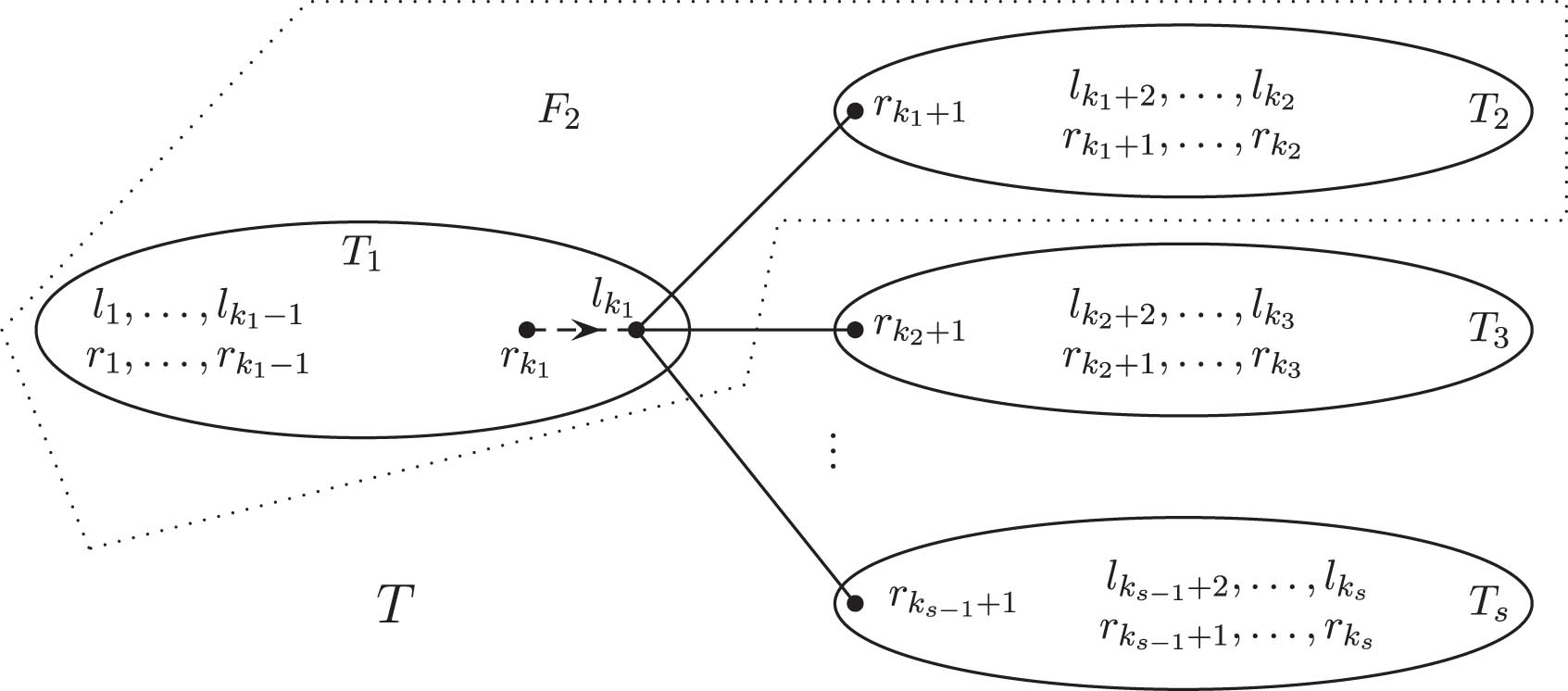
Consider the tree T with a matching edge [ l k 1 , r k 1 ] (Figure 1). Let the degree of l k 1 be s , s ≥ 1 . Let r k 1 + 1 , r k 2 + 1 , … , r k s − 1 + 1 be some distinct vertices other than r k 1 that are adjacent to l k 1 . Note that when we delete the edges [ l k 1 , r k 1 + 1 ] , … , [ l k 1 , r k s − 1 + 1 ] , we obtain s many smaller nonsingular trees, say T 1 , … , T s . Assume that the vertex set of T 1 is { l 1 , … , l k 1 , r 1 , … , r k 1 } , the vertex set of T 2 is { l k 1 + 1 , … , l k 2 , r k 1 + 1 , … , r k 2 } , and so on up to the vertex set of T s is { l k s − 1 + 1 , … , l k s , r k s − 1 + 1 , … , r k s } . Let us put an arrow on the edge [ l k 1 , r k 1 ] from r k 1 to l k 1 . This arrow indicates that, from a vertex r i in T 2 , we do not have an alternating path to a vertex in T 1 . Similarly, from a vertex r i in T 3 , we do not have an alternating path to a vertex in T 1 , T 2 , T 4 , T 5 , … , T s . Similar statements are true for vertices r i in T 4 , … , T s . Also, from a vertex l i in T 1 , we only have alternating paths to vertices in T 1 but not to a vertex in T 2 , … , T s . Let us take F 1 be the tree T 1 . For i = 2 , … , s , let F i be the subtree of T obtained by taking F i − 1 and T i and by inserting the edge [ l k 1 , r k i − 1 + 1 ] . Clearly, F s is the original tree T .

(a) Let μ l k 1 be the signed degree vector at l k 1 of T 1 , and let μ be the signed degree vector at l k 1 of T . Then, μ = μ l k 1 0 t .

(b) Let L ( F i ) be the bipartite Laplacian matrix of F i for i = 1 , … , s and L ( T i ) be the bipartite Laplacian matrix of T i for i = 1 , … , s . Clearly, L ( T 1 ) = L ( F 1 ) . Let μ r k i + 1 be the signed degree vector at r k i + 1 of T i + 1 , for i = 1 , … , s − 1 . By E i j we denote the matrix of an appropriate size with 1 at position ( i , j ) and 0 elsewhere. Then, for i = 2 , … , s , we have

L ( F i ) = L ( T 1 ) + ( i − 1 ) μ l k 1 e k 1 t − μ l k 1 μ r k 1 + 1 t ⋯ − μ l k 1 μ r k i − 1 + 1 t − E 1 k 1 L ( T 2 ) + e 1 μ r k 1 + 1 t ⋯ 0 ⋮ 0 ⋱ 0 − E 1 k 1 0 ⋯ L ( T i ) + e 1 μ r k i − 1 + 1 t .

In particular,

L ( T ) = L ( T 1 ) + ( s − 1 ) μ l k 1 e k 1 t − μ l k 1 μ r k 1 + 1 t ⋯ − μ l k 1 μ r k s − 1 + 1 t − E 1 k 1 L ( T 2 ) + e 1 μ r k 1 + 1 t ⋯ 0 ⋮ 0 ⋱ 0 − E 1 k 1 0 ⋯ L ( T s ) + e 1 μ r k s − 1 + 1 t

We illustrate the above remark by the following example.

$Figure 1 Understanding L ( T ) {\mathfrak{L}}\left(T) .$

Figure 1

Understanding L ( T ) .

Example 15

Consider the tree T , as shown in Figure 2. Edges in the perfect matching are shown as dashed lines.

Note that [ l 3 , r 3 ] is a matching edge, and the other vertices that are adjacent to l 3 are r 4 , r 7 . Consider k 1 = 3 , k 2 = 6 , and k 3 = 8 in Remark 14. Note that T 1 , T 2 , and T 3 are nonsingular trees with the vertex set { l 1 , l 2 , l 3 , r 1 , r 2 , r 3 } , { l 4 , l 5 , l 6 , r 4 , r 5 , r 6 } , and { l 7 , l 8 , r 7 , r 8 } , respectively. Furthermore, F 2 is a subtree of T induced by { l 1 , … , l 6 , r 1 , … , r 6 } and F 3 is a subtree of T induced by { l 1 , l 2 , l 3 , l 7 , l 8 , r 1 , r 2 , r 3 , r 7 , r 8 } . We set F 1 = T 1 .

Let μ l 3 be the signed degree vector at l 3 of T 1 , let μ r 4 be the signed degree vector at r 4 of T 2 , and let μ r 7 be the signed degree vector at r 7 of T 3 . Note that

μ l 3 = − 1 − 1 3 t , μ r 4 = 2 − 1 0 t , and μ r 7 = 2 − 1 t

Let μ be the signed degree vector at l 3 of T . Then,

μ = − 1 − 1 3 0 0 0 0 0 t = μ l 3 0 t .

Let L ( T i ) be the bipartite Laplacian matrix of T i for i = 1 , 2 , 3 . Then, we see that

L ( T 1 ) = 1 0 − 1 0 1 − 1 − 1 − 1 2 and L ( T 2 ) = 3 − 2 − 1 − 1 1 0 − 2 1 1 and L ( T 3 ) = 1 − 1 − 1 1

Note that

L ( F 2 ) = 1 0 − 2 2 − 1 0 0 1 − 2 2 − 1 0 − 1 − 1 5 − 6 3 0 0 0 − 1 5 − 3 − 1 0 0 0 − 1 1 0 0 0 0 − 2 1 1 = L ( T 1 ) + μ l 3 e 3 t μ l 3 − 2 1 0 − E 13 L ( T 2 ) + e 1 μ r 4 t = L ( T 1 ) + μ l 3 e 3 t − μ l 3 μ r 4 t − E 13 L ( T 2 ) + e 1 μ r 4 t .

In a similar way, we can see that

L ( F 3 ) = 1 0 − 3 2 − 1 0 2 − 1 0 1 − 3 2 − 1 0 2 − 1 − 1 − 1 8 − 6 3 0 − 6 3 0 0 − 1 5 − 3 − 1 0 0 0 0 0 − 1 1 0 0 0 0 0 0 − 2 1 1 0 0 0 0 − 1 0 0 0 3 − 2 0 0 0 0 0 0 − 1 1 = L ( T 1 ) + 2 μ l 3 e 3 t − μ l 3 μ r 4 t − μ l 3 μ r 7 t − E 13 L ( T 2 ) + e 1 μ r 4 t 0 − E 13 0 L ( T 2 ) + e 1 μ r 7 t

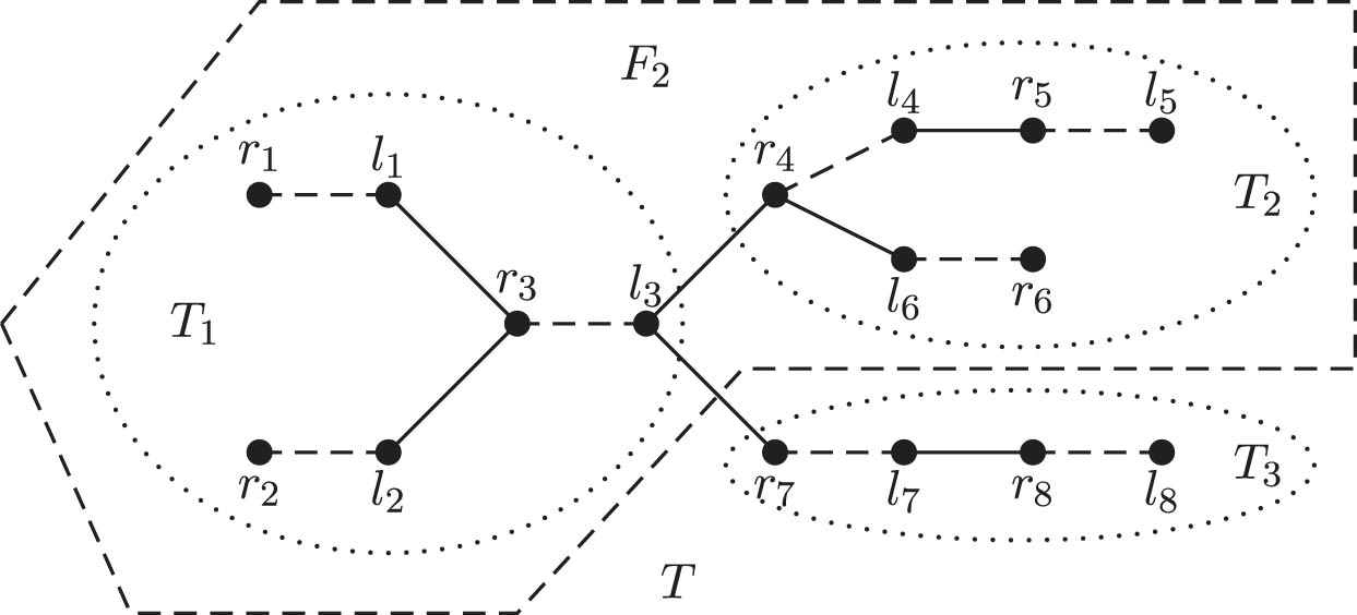
Grone et al. [17, Theorem 2.1] have mentioned about the integer eigenvalues λ > 1 of the usual Laplacian matrix of tree T . The following is an extension of it to the bipartite Laplacian matrix of a nonsingular tree.

Figure 2

Illustration of Remark 14.

Theorem 16

Let T be a nonsingular tree on 2 p vertices. Suppose λ is an integer eigenvalue of the L ( T ) with a corresponding eigenvector u . Then, the following assertions hold.

If λ ≠ 0 , ± 1 , then λ divides p .
If λ ≠ ± 1 , then no coordinate of u is zero.
If λ ≠ ± 1 , then the geometric multiplicity of λ is one.

Proof of Item (a). By part (a) of Theorem 9, the characteristic polynomial χ ( x ) ≔ det ( x I − L ( T ) ) = x f ( x ) , where f ( x ) is some polynomial with integer coefficients. By item (b) of Theorem 9,

f ( 0 ) = coefficient of x in χ ( x ) = ( − 1 ) p − 1 × ( sum of the principal minors of L ( T ) of size p − 1 ) = ( − 1 ) p − 1 p .

Suppose λ ≠ 0 , ± 1 . It follows that χ ( λ ) = 0 and hence f ( λ ) = 0 . As each term of f ( λ ) is a multiple of λ except f ( 0 ) , we see that λ divides f ( 0 ) . The result now follows.

Proof of Item (b). Suppose λ ≠ ± 1 . Note that if T = P 2 , then u = [ 1 ] and the result holds for p = 1 . Let us assume T be a tree on 2 p vertices, p > 1 . By way of contradiction, assume that some u ( k ) = 0 . In that case, either (i) d ( l k ) ≥ 2 or (ii) d ( l k ) = 1 and d ( r k ) ≥ 2 .

Let us first assume that case (i) holds. In this case, we locate the matching edge [ l k , r k ] in T . Imagine deleting all nonmatching edges at the vertex l k . This will create at least two components, and one of which contains the matching edge [ l k , r k ] .

Recall that, if we relabel the vertices inside L , and call the resulting tree T ′ , then L ( T ′ ) is permutation similar to L ( T ) , and hence λ will remain an eigenvalue of L ( T ′ ) with a corresponding eigenvector u ′ having a zero entry.

In view of this, we assume that T is already labeled as shown in Remark 14 and that u ( k 1 ) = 0 . That is, when we delete the nonmatching edges at l k 1 we have s many components T 1 , T 2 , … , T s , where the component T 1 has the vertex set { l 1 , r 1 , … , l k 1 , r k 1 } , the component T 2 has the vertex set { l k 1 + 1 , r k 1 + 1 , … , l k 2 , r k 2 } , and so on.

Now, we partition the eigenvector conformally u = [ u 1 ⋯ u s ] t . Observe that u 1 ( k 1 ) = u ( k 1 ) = 0 and

L ( T 1 ) + ( s − 1 ) μ l k 1 e k 1 t − μ l k 1 μ r k 1 + 1 t ⋯ − μ l k 1 μ r k s − 1 + 1 t − E 1 k 1 L ( T 2 ) + e 1 μ r k 1 + 1 t ⋯ 0 ⋮ 0 ⋱ 0 − E 1 k 1 0 ⋯ L ( T s ) + e 1 μ r k s − 1 + 1 t u 1 ⋮ u s = λ u 1 ⋮ u s

If all u i = 0 for i = 2 , … , s , then u 1 ≠ 0 . It follows that L ( T 1 ) u 1 = λ u 1 . We may use the induction hypothesis to conclude that no coordinate of u 1 is zero. This is a contradiction as u 1 ( k 1 ) = 0 . Therefore, at least one of u 2 , … , u s is nonzero, say u 2 ≠ 0 . Then, we have Z u 2 = λ u 2 , where Z = L ( T 2 ) + e 1 μ r k 1 + 1 t . Let C be the matrix obtained from L ( T 2 ) by replacing the first row by μ r k 1 + 1 t . Note that det Z = det L ( T 2 ) + det C . By expanding the determinant of C along the first row, we see that

det C = ∑ i ( − 1 ) 1 + i μ r k 1 + 1 ( i ) det L ( T 2 ) ( 1 ∣ i ) .

By part (b) of Theorem 9, ( − 1 ) 1 + i det L ( T 2 ) ( 1 ∣ i ) = 1 . Therefore, by Lemma 7, det C = 1 t μ r k 1 + 1 = 1 . Since det L ( T 2 ) = 0 , it follows that det Z = 1 . Let f ( x ) = det ( x I − Z ) be the characteristic polynomial of Z . Then, f ( x ) is a monic polynomial (with integer coefficients) such that f ( 0 ) = ± 1 . Therefore, the only possible rational eigenvalues of Z are 1 and − 1 . Thus, we arrived at a contradiction as λ ≠ ± 1 .

Now we consider the case (ii). Assume that d ( r k ) = m + 1 ≥ 2 and d ( l k ) = 1 . Let v 1 , … , v m be the vertices other than l k that are adjacent to r k . Let T 1 , … , T m be nonsingular subtrees of T obtained by deleting the edges [ r k , v 1 ] , … , [ r k , v m ] and that do not contain the edge [ l k , r k ] . Let us assume that the vertex set of T 1 is { l 1 , … , l k − 1 , r 1 , … , r k − 1 } , the vertex set of T 2 is { l k + 1 , … , l k + t 1 , r k + 1 , … , r k + t 1 } , and so on up to the vertex set of T m is { l k + t m − 2 + 1 , … , l k + t m − 1 , r k + t m − 2 + 1 , … , r k + t m − 1 } .

Let us partition u = [ u 1 u ( k ) u 2 ⋯ u m ] t . Since u is an eigenvector and u ( k ) = 0 , it follows that among u 1 , … , u m , at least one them is a nonzero vector, say u 1 ≠ 0 . Without loss of any generality, let us assume that v 1 = l 1 . Note that from a vertex r i in T 1 , we do not have an alternating path to a vertex in T 2 , … , T m . Further note that d T ( v ) = d T 1 ( v ) for each v ∈ T 1 − l 1 . It follows that

L ( T 1 ) + μ l 1 e 1 t − μ l 1 0 − e 1 t m ∗ ∗ ∗ ∗ u 1 u ( k ) u ¯ = λ u 1 u ( k ) u ¯ ,

where u ¯ = [ u 2 ⋯ u m ] t . Note that X u 1 = λ u 1 , where X = L ( T 1 ) + μ l 1 e 1 t . Let Y be the matrix obtained from L ( T 1 ) by replacing the first column by μ l 1 t . Note that det X = det L ( T 1 ) + det Y . By expanding the determinant of Y along the first column, we see that

det Y = ∑ i ( − 1 ) 1 + i μ l 1 ( i ) det L ( T 1 ) ( i ∣ 1 ) .

By part (b) of Theorem 9, ( − 1 ) 1 + i det L ( T 1 ) ( i ∣ 1 ) = 1 . Therefore, by Lemma 7 det X = 1 t μ l 1 = 1 . Since det L ( T 1 ) = 0 , it follows that det X = 1 . Let g ( x ) = det ( x I − X ) be the characteristic polynomial of X . Then, g ( x ) is a monic polynomial (with integer coefficients) such that g ( 0 ) = ± 1 . Therefore, the only possible rational eigenvalues of X are 1 and − 1 . Thus, we arrived at a contradiction as λ ≠ ± 1 . This completes the proof.

Proof of Item (c). It directly follows from item (b).

We close this section by supplying two observations about the eigenvalues of the bipartite Laplacian matrix of a path.

Lemma 17

Let T be a path on 2 p vertices with a standard vertex bipartition ( L , R ) . Let λ be an eigenvalue of the bipartite Laplacian matrix of T. Then, the following assertions hold.

The geometric multiplicity of λ is one.
λ = 2 is an eigenvalue of L ( T ) if and only if p = 2 k , for some k .

Proof of Item (a). It follows from Theorem 13.

Proof of Item (b). Suppose p = 2 k . Consider the vector u as follows:

u = [ 1 − 1 − 3 3 3 2 − 3 2 ⋯ ( − 1 ) k − 1 3 k − 1 ( − 1 ) k 3 k − 1 ] t .

Then, L ( T ) u = 2 u . The converse of the result follows from Theorem 16.

3 The inverse of the bipartite distance matrix

In this section, first, we recall some terminologies from the work of Bapat et al. [4], and using them, we present a formula for the inverse of the bipartite distance matrix of a nonsingular tree.

Let T be a nonsingular tree on 2 p vertices with a standard vertex bipartition ( L , R ) . Recall that, an alternating path is called an even alternating path if it has an even number of matching edges, otherwise it is called an odd alternating path. Let A T , v + denote the set of all even alternating paths in T that start at v . Similarly, we denote the set of all odd alternating paths in T that start at v by A T , v − . By diff T ( v ) , we mean the quantity diff T ( v ) ≔ ∣ A T , v + ∣ − ∣ A T , v − ∣ . The vector τ ( T ) , or simply τ , of size 2 p is defined by τ ( v ) ≔ 1 − d T ( v ) [ 1 + diff T ( v ) ] for each v in T . The entries of τ are ordered according to l 1 , … , l p , r 1 , … , r p . By τ r ( T ) , or simply by τ r , we mean the restriction of τ ( T ) on R . Similarly, by τ l ( T ) , or simply by τ l , we mean the restriction of τ ( T ) on L . For the tree T in Example 4, note that

τ r ( T ) = 1 − 2 1 0 1 t and τ l ( T ) = 1 − 1 − 1 1 1 t .

The next result relates the structures the τ r vectors of the new tree with that of the old one under attaching a new P 2 at a vertex. The first item was proved in [4, Lemma 3.4], and the proof of the second item is routine.

Lemma 18

Let T be a nonsingular tree on 2 p vertices with a standard vertex bipartition ( L , R ) . Let T ^ be the tree obtained from T by attaching a new P 2 at v .

If v = r k for some k, then τ r ( T ^ ) = τ r ( T ) 0 − ( 1 + diff T ( v ) ) e k − 1 .
If v = l k for some k , then τ r ( T ^ ) = τ r ( T ) 1 + μ v ( T ) 0 , where μ v ( T ) is the signed degree vector at v of T .

Let T be a nonsingular tree on 2 p vertices. Recall that, the factor bd ( T ) ≔ det B ( T ) ∕ ( − 2 ) p − 1 is called the bipartite distance index of T . The following result was proved in [4, Theorem 3.7], which relates the bipartite distance index of the new tree to that of the old one under the operation of attaching a new P 2 at a vertex.

Lemma 19

[4, Theorem 3.7] Let T be a nonsingular tree on 2 p vertices and let v be a vertex in T. Let T ^ be the tree obtained from T by attaching a new P 2 at v . Then, bd ( T ^ ) = bd ( T ) + 2 [ 1 + diff T ( v ) ] .

The following properties of τ r and τ l were proved in [4].

Theorem 20

[4, Lemma 3.5, Theorem 3.7, Corollary 3.8] Let T be a nonsingular tree on 2 p vertices with a standard vertex bipartition ( L , R ) . Let B be the bipartite distance matrix of T and let τ r ( T ) , τ l ( T ) be the restriction of τ ( T ) on R , L , respectively. Then, 1 T τ r = 1 and 1 t τ l = 1 . Furthermore,

B ( T ) τ r ( T ) = bd ( T ) 1 and τ l t ( T ) B ( T ) = bd ( T ) 1 t

It was proved in [4] that the bipartite distance matrix of a nonsingular tree is always invertible.

Theorem 21

[4, Corollary 4.2] Let T be a nonsingular tree on 2 p vertices with a standard vertex bipartition ( L , R ) . Then, bd ( T ) is an odd number. In particular, B ( T ) is invertible.

Our next aim is to find a formula for the inverse of the bipartite distance matrix of a nonsingular tree. Let us first examine the relationship between the bipartite distance matrix and the bipartite Laplacian matrix of a nonsingular tree.

Lemma 22

Let T be a nonsingular tree on 2 p vertices with a standard vertex bipartition ( L , R ) . Let B ( T ) and L ( T ) be the bipartite distance matrix and the bipartite Laplacian matrix of T, respectively. Let τ r ( T ) be the restriction of τ ( T ) on R. Then,

− L ( T ) B ( T ) + 2 τ r ( T ) 1 t = 2 I .

Proof

We proceed by induction on p . Let p = 1 . Then, T = P 2 , L ( T ) = [ 0 ] , and τ r ( T ) = [ 1 ] . It follows that − L ( T ) B ( T ) + 2 τ r ( T ) 1 t = 2 . Let p = 2 . Then, T = P 4 . Let P 4 = [ l 1 , r 1 , l 2 , r 2 ] . Then, L ( T ) = 1 − 1 − 1 1 and τ r ( T ) = 1 0 t . It follows that

− L ( T ) B ( T ) + 2 τ r ( T ) 1 t = − 1 − 1 − 1 1 1 3 1 1 + 2 2 0 0 = 2 I .

Assume the result is true for p . Let T ^ be the nonsingular tree on 2 p + 2 vertices. Then, T ^ is obtained from some nonsingular tree T on 2 p vertices by attaching a new P 2 at some vertex v . Let μ be the signed degree vector at v of T . Note that either v ∈ L or v ∈ R .

Let us first consider that v = l k for some 1 ≤ k ≤ p . By item (a) of Lemma 6, we have

L ( T ^ ) = L ( T ) + μ e k t − μ − e k t 1 .

Let x be a vector of size p such that x ( i ) = dist ( l i , r p + 1 ) for each i = 1 , … , p . Then, the bipartite distance matrix of T ^ can be written as follows:

B ( T ^ ) = B ( T ) x e k t B ( T ) + 2 1 t 1 .

Now note that

(1) L ( T ^ ) B ( T ^ ) = L ( T ) + μ e k t − μ − e k t 1 B ( T ) x e k t B ( T ) + 2 1 t 1 = L ( T ) B ( T ) + μ e k t B ( T ) − μ e k t B ( T ) − 2 μ 1 t L ( T ) x + μ e k t x − μ − e k t B ( T ) + e k t B ( T ) + 2 1 t − e k t x + 1 = L ( T ) B ( T ) − 2 μ 1 t L ( T ) x 2 1 t 0 .

The last equality follows from the fact that e k t x = x ( k ) = dist ( l k , r p + 1 ) = 1 . By item (b) of Lemma 18, we have

τ r ( T ^ ) = τ r ( T ) 1 + − μ 0 .

By the induction hypothesis, we obtain

(2) L ( T ) B ( T ) = 2 τ r ( T ) 1 t − 2 I .

It follows from (1) that

− L ( T ^ ) B ( T ^ ) + 2 τ r ( T ^ ) 1 t = − 2 τ r ( T ) 1 t − 2 I − 2 μ 1 t L ( T ) x 2 1 t 0 + 2 ( τ r ( T ) − μ ) 1 t 2 1 t = 2 I − L ( T ) x + 2 ( τ r ( T ) − μ ) 0 2 .

Therefore, in order to complete the proof for the v = l k case, we only need to show that L ( T ) x = 2 ( τ r ( T ) − μ ) .

Let the degree of l k in T be s , ( s ≥ 1 ). Let T 1 be the tree obtained from T by removing all vertices adjacent to l k except the vertex r k . If s = 1 , then T 1 is the same as T . Without loss of any generality, let us assume that T 1 has the vertex set { l 1 , r 1 , … , l k − 1 , r k − 1 , l k , r k } . Let μ ^ be the signed degree vector at v of T 1 . By Remark 14, μ = μ ^ 0 t . In addition, note that

(3) x = B ( T ) e k + 2 ⋯ 2 0 0 ⋯ 0 t ,

where the entries 2 in the last vector are for the vertices l 1 , … , l k − 1 . Let z be a vector of size ( p − k ) defined as follows. For i = 1 , … , ( p − k ) , z ( i ) = − 1 if r k + i is adjacent to l k and z ( i ) = 0 otherwise. Hence, by Remark 14, we have

(4) L ( T ) 2 ⋯ 2 0 0 ⋯ 0 t = L ( T 1 ) + ( s − 1 ) μ ^ e k t ∗ z e k t ∗ 2 ( 1 − e k ) 0 = 2 L ( T 1 ) 1 + ( s − 1 ) μ ^ z − 2 L ( T 1 ) e k + ( s − 1 ) μ ^ z = − 2 L ( T 1 ) e k 0 = − 2 μ ^ − e k 0 = − 2 μ + 2 e k [ By Remark 14 ] .

From equations (2)–(4), it follows that L ( T ) x = 2 ( τ r ( T ) − μ ) . This completes the proof of the case v = l k .

Now we consider the case v = r k for some 1 ≤ k ≤ p . By item (b) of Lemma 6, we have

L ( T ^ ) = L ( T ) + e k μ t − e k − μ t 1 .

Let y be a vector of size p such that y ( i ) = dist ( r i , l p + 1 ) for each i = 1 , … , p . Then, the bipartite distance matrix of T ^ can be written as follows:

B ( T ^ ) = B ( T ) B ( T ) e k + 21 y t 1 .

By using the facts L ( T ) 1 = 0 and μ t 1 = 1 , we obtain

(5) L ( T ^ ) B ( T ^ ) = L ( T ) + e k μ t − e k − μ t 1 B ( T ) B ( T ) e k + 21 y t 1 = L ( T ) B ( T ) + e k ( μ t B ( T ) − y t ) L ( T ) B ( T ) e k + e k μ t B ( T ) e k + e k − ( μ t B ( T ) − y t ) − μ t B ( T ) e k − 1 .

We claim that the following identity is true:

(6) y t − μ t B ( T ) = 2 [ 1 + diff T ( v ) ] 1 t .

In order to verify our claim, suppose the degree of r k in T is m , ( m ≥ 1 ). Let T 0 be the tree obtained from T by removing all vertices adjacent to l k except the vertex r k . If m = 1 , then T 0 is same as T .

Without loss of any generality, assume that T 0 has the vertex set { l 1 , r 1 , … , l k − 1 , r k − 1 , l k , r k } . Now note that

(7) y t = e k t B ( T ) + 2 ⋯ 2 0 0 ⋯ 0 t ,

where the entries 2 in the last vector are for the vertices r 1 , … , r k − 1 .

Let l k 1 , … , l k m − 1 be the vertices other than l k that are adjacent to r k . Let T i be the component of T − r k that contains the vertex l k i but does not contain the vertex l k , for i = 1 , … , m − 1 . For i = 1 , … , m − 1 , we have

e k t B ( T ) − e k i t B ( t ) = − 2 ⋯ − 2 0 0 ⋯ 0 t + z i ,

where the entries − 2 in the first vector are for the vertices r 1 , … , r k − 1 , and z i is a vector of size p such that z i ( j ) = 2 if r j ∈ T i and z i ( j ) = 0 otherwise. Therefore, it follows that

( m − 1 ) e k t B ( T ) − ∑ i = 1 m − 1 e k i t B ( t ) = − 2 ( m − 1 ) ⋯ − 2 ( m − 1 ) 0 2 ⋯ 2 t .

Now note that

e k t L ( T ) = m μ t − e k t − e k 1 t − ⋯ − e k m − 1 t .

Therefore, we obtain

(8) e k t L ( T ) B ( T ) + m e k t B ( T ) = m μ t B ( T ) + ( m − 1 ) e k t B ( T ) − ∑ i = 1 m − 1 e k i t B ( t ) = m μ t B ( T ) + − 2 ( m − 1 ) ⋯ − 2 ( m − 1 ) 0 2 ⋯ 2 t = m μ t B ( T ) + 2 1 t − 2 e k t − m 2 ⋯ 2 0 0 ⋯ 0 t ,

where the entries 2 in the last vector are for the vertices r 1 , … , r k − 1 . By equations (7) and (8), we see that

e k t L ( T ) B ( T ) = m μ t B ( T ) + 2 1 t − 2 e k t − m y t .

Let b = 1 + diff T ( r k ) . Then, τ r ( k ) = 1 − m b . By applying induction hypothesis, we obtain

e k t L ( T ) B ( T ) = 2 τ r ( k ) 1 t − 2 e k t = 2 1 t − 2 e k t − 2 m b 1 t .

It follows that m μ t B ( T ) = m y t − 2 m b 1 t , and our claim is established.

Now we will use the identity (6) to complete the remaining part of the proof. First, note that μ t B ( T ) e k = y ( k ) − 2 b = 1 − 2 b . By using the identities (6) and (2) in equation (5), we obtain

(9) L ( T ^ ) B ( T ^ ) = L ( T ) B ( T ) − 2 b e k 1 t L ( T ) B ( T ) e k + ( 1 − 2 b ) e k + e k − 2 b 1 t − 2 + 2 b = 2 τ r ( T ) 1 t − 2 I − 2 b e k 1 t 2 τ r ( T ) 1 t e k − 2 b e k 2 b 1 t − 2 + 2 b

From item (a) of Lemma 18,

2 τ r ( T ^ ) 1 t = 2 τ r ( T ) 1 t − 2 b e k t 1 t 2 b 1 t .

Hence, the result follows by using the above identity in equation (9).□

The following result is an immediate consequence of Lemma 22.

Lemma 23

Let T be a nonsingular tree on 2 p vertices with a standard vertex bipartition ( L , R ) . Let B ( T ) and L ( T ) be the bipartite distance matrix and the bipartite Laplacian matrix of T, respectively. Let τ l ( T ) be the restriction of τ ( T ) on L . Then,

− B ( T ) L ( T ) + 21 τ l t ( T ) = 2 I .

We are now in a position to supply a formula for the inverse of the bipartite distance matrix of a nonsingular tree T . This is one of our main results.

Theorem 24

Let T be a nonsingular tree on 2 p vertices with a standard vertex bipartition ( L , R ) . Let B ( T ) and L ( T ) be the bipartite distance matrix and the bipartite Laplacian matrix of T, respectively. Let τ r ( T ) and τ l ( T ) be the restriction of τ ( T ) on R and L , respectively. Then,

B ( T ) − 1 = − 1 2 L ( T ) + 1 bd ( T ) τ r ( T ) τ l t ( T ) .

Proof

By using Lemmas 20 and 22, we have

− 1 2 L ( T ) + 1 bd ( T ) τ r ( T ) τ l t ( T ) B ( T ) = 1 2 ( − L ( T ) B ( T ) + 2 τ r ( T ) 1 t ) = I .

This completes the proof.□

Recall that, for the usual distance matrix D of a tree T , Russell Merris in [20, Corollary 2] showed that the multiplicity of the eigenvalue − 2 of D is at least p ( T ) − q ( T ) − 1 . In the following result, we observe that a similar fact is also true for the bipartite distance matrix of a nonsingular tree.

Corollary 25

Let T be a nonsingular tree on 2 p ( p > 1 ) vertices with a standard vertex bipartition ( L , R ) . Let B be the bipartite distance matrix of T. If − 2 is an eigenvalue of B , then the geometric multiplicity of − 2 is at least P ( T ) − Q ( T ) .

Proof

Let L be the bipartite Laplacian matrix of T . If P ( T ) − Q ( T ) = 0 , then there is nothing to prove. Let us assume P ( T ) − Q ( T ) > 1 . Let w be a root of at least two pendant-two-paths. Without loss of any generality, let us assume that w ∈ L . Let [ l k 1 , r k 1 , w ] , … , [ l k m , r k m , w ] be pendant-two-paths at w . By Theorem 12, we noted that e k i − e k j , 1 ≤ i < j ≤ m , are eigenvectors of L corresponding to the eigenvalue 1. Now note that, for i , j = 1 , … , m , we have

τ l ( k i ) = τ l ( k j ) and τ r ( k i ) = τ r ( k j ) .

The remaining part of the proof follows from Theorem 24.□

4 Conclusion

In this document, a generalization of the usual Laplacian matrix of a tree called the bipartite Laplacian matrix has been introduced. It was shown that it enjoys many proprieties that are true for the usual Laplacian matrix. There are two properties of the bipartite Laplacian matrix of a nonsingular tree that we believe are true, but we do not have complete proof. We mention them below.

Conjecture 1

Let L be a bipartite Laplacian matrix of a nonsingular tree T . Then, all eigenvalues of L are nonnegative real numbers.

Conjecture 2

Let L be a bipartite Laplacian matrix of a nonsingular tree T . Then, L is diagonalizable.

In addition, Jana [18] has considered the q -analogue variations of the bipartite distance matrix for nonsingular trees and generalized Theorem 1. It would be intriguing to explore the inverse of q -analogue variations of bipartite distance matrix as well.

Acknowledgements

The authors express their heartfelt gratitude to the editor and two anonymous referees for providing valuable feedback and insightful comments on the manuscript. Their input has improved the quality and clarity of the article.

Funding information: R. B. Bapat acknowledges the support of the Indian National Science Academy (INSA), New Delhi, India, under the INSA Senior Scientist scheme. R. Jana was supported by the fellowship of Indian Institute of Technology Guwahati (IIT Guwahati).
Conflict of interest: There is no conflict of interest.
Data availability statement: Data sharing is not applicable to this article as no datasets were generated or analyzed during this study.

References

[1] M. Aouchiche and P. Hansen, Two Laplacians for the distance matrix of a graph, Linear Algebra Appl. 439 (2013), no. 1, 21–33. 10.1016/j.laa.2013.02.030Suche in Google Scholar

[2] R. Bapat, Determinant of the distance matrix of a tree with matrix weights, Linear Algebra Appl. 416 (2006), no. 1, 2–7. 10.1016/j.laa.2005.02.022Suche in Google Scholar

[3] R. Bapat, Graphs and Matrices, Universitext, Springer London, 2014. 10.1007/978-1-4471-6569-9Suche in Google Scholar

[4] R. Bapat, R. Jana, and S. Pati, The bipartite distance matrix of a nonsingular tree, Linear Algebra Appl. 631 (2021), 254–281. 10.1016/j.laa.2021.09.001Suche in Google Scholar

[5] R. Bapat, S. J. Kirkland, and M. Neumann, On distance matrices and Laplacians, Linear Algebra Appl. 401 (2005), 193–209. 10.1016/j.laa.2004.05.011Suche in Google Scholar

[6] R. Bapat, A. K. Lal, and S. Pati, A q-analogue of the distance matrix of a tree, Linear Algebra Appl. 416 (2006), 2–3, 799–814. 10.1016/j.laa.2005.12.023Suche in Google Scholar

[7] R. Bapat and S. Sivasubramanian, Squared distance matrix of a tree: Inverse and inertia, Linear Algebra Appl. 491 (2016), 328–342. 10.1016/j.laa.2015.09.008Suche in Google Scholar

[8] R. B. Bapat, Squared distance matrix of a weighted tree, Electron. J. Graph Theory Appl. (EJGTA) 7 (2019), no. 2, 301–313. 10.5614/ejgta.2019.7.2.8Suche in Google Scholar

[9] R. B. Bapat and S. Sivasubramanian, The arithmetic Tutte polynomial of two matrices associated to trees, Special Matrices 6 (2018), 310–322. 10.1515/spma-2018-0026Suche in Google Scholar

[10] J. A. Bondy and U. S. R. Murty, Graph theory, Number 244 in Graduate Texts in Mathematics, Springer-Verlag, London, New York, 2008. 10.1007/978-1-84628-970-5Suche in Google Scholar

[11] D. Cvetkovic, D. Cvetković, M. Doob, and H. Sachs, Spectra of graphs: Theory and application, Pure and applied mathematics : A series of monographs and textbooks. Academic Press, Cambridge, 1980. Suche in Google Scholar

[12] I. Faria, Permanental roots and the star degree of a graph, Linear Algebra Appl. 64 (1985), 255–265. 10.1016/0024-3795(85)90281-2Suche in Google Scholar

[13] C. D. Godsil, Inverses of trees, Combinatorica 5 (1985), no. 1, 33–39. 10.1007/BF02579440Suche in Google Scholar

[14] R. L. Graham, A. J. Hoffman, and H. Hosoya, On the distance matrix of a directed graph, J. Graph Theory 1 (1977), no. 1, 85–88. 10.1002/jgt.3190010116Suche in Google Scholar

[15] R. L. Graham and L. Lovasz, Distance matrix polynomials of trees, Adv. Math. 29 (1978), no. 1, 60–88. 10.1016/0001-8708(78)90005-1Suche in Google Scholar

[16] R. L. Graham and H. O. Pollak, On the addressing problem for loop switching, Bell Sys. Tech. J. 50 (1971), no. 8, 2495–2519. 10.1002/j.1538-7305.1971.tb02618.xSuche in Google Scholar

[17] R. Grone, R. Merris, and V. S. Sunder, The Laplacian spectrum of a graph, SIAM J. Matrix Anal. Appl. 11 (1990), no. 2, 218–238. 10.1137/0611016Suche in Google Scholar

[18] R. Jana, A q-analogue of the bipartite distance matrix of a nonsingular tree, Discrete Math. 346 (2023), no. 1, 113153. 10.1016/j.disc.2022.113153Suche in Google Scholar

[19] H. Kurata and R. B. Bapat, Moore-Penrose inverse of a hollow symmetric matrix and a predistance matrix, Special Matrices 4 (2016), 270–282.10.1515/spma-2016-0028Suche in Google Scholar

[20] R. Merris, The distance spectrum of a tree, J. Graph Theory 14 (1990), no. 3, 365–369. 10.1002/jgt.3190140309Suche in Google Scholar

[21] C. Reinhart, The normalized distance Laplacian, Special Matrices 9 (2021), 1–18. 10.1515/spma-2020-0114Suche in Google Scholar

[22] Y. Yang and D. Ye, Inverses of bipartite graphs, Combinatorica 38 (2017), no. 5, 1251–1263. 10.1007/s00493-016-3502-ySuche in Google Scholar

[23] H. Zhou, The inverse of the distance matrix of a distance well-defined graph, Linear Algebra Appl. 517 (2017), 11–29. 10.1016/j.laa.2016.12.008Suche in Google Scholar

[24] H. Zhou and Q. Ding, The distance matrix of a tree with weights on its arcs, Linear Algebra Appl. 511 (2016), 365–377. 10.1016/j.laa.2016.09.028Suche in Google Scholar

Received: 2023-03-08

Revised: 2023-07-24

Accepted: 2023-08-01

Published Online: 2023-08-27

This work is licensed under the Creative Commons Attribution 4.0 International License.

Artikel in diesem Heft

https://doi.org/10.1515/spma-2023-0102

Schlagwörter für diesen Artikel

tree; distance matrix; Laplacian matrix; bipartite distance matrix; bipartite Laplacian matrix

Creative Commons

BY 4.0