Quantum motion control for packaging machines

2.1 Description of the architecture

The architecture of a motion control system is based on a system called “axis control” which is described in detail in Figure 1 and which consists of the following elements:

1. A motion controller unit 100 characterized by the following three sub-units:

   1. A logic control unit 101, typically defined as programmable logic controller (Plc), is used for developing the required programmed logic steps, necessary to control the axes in the different motion situations: during the production, when some trouble is verified, etc.

   2. A function unit 102 for generating a motion profile, having the task of generating a reference profile for the movement;

   3. A position controller unit 103 for generating set points (for motion profile in closed-loop systems) to close a position/velocity feedback loop;

Figure 1:

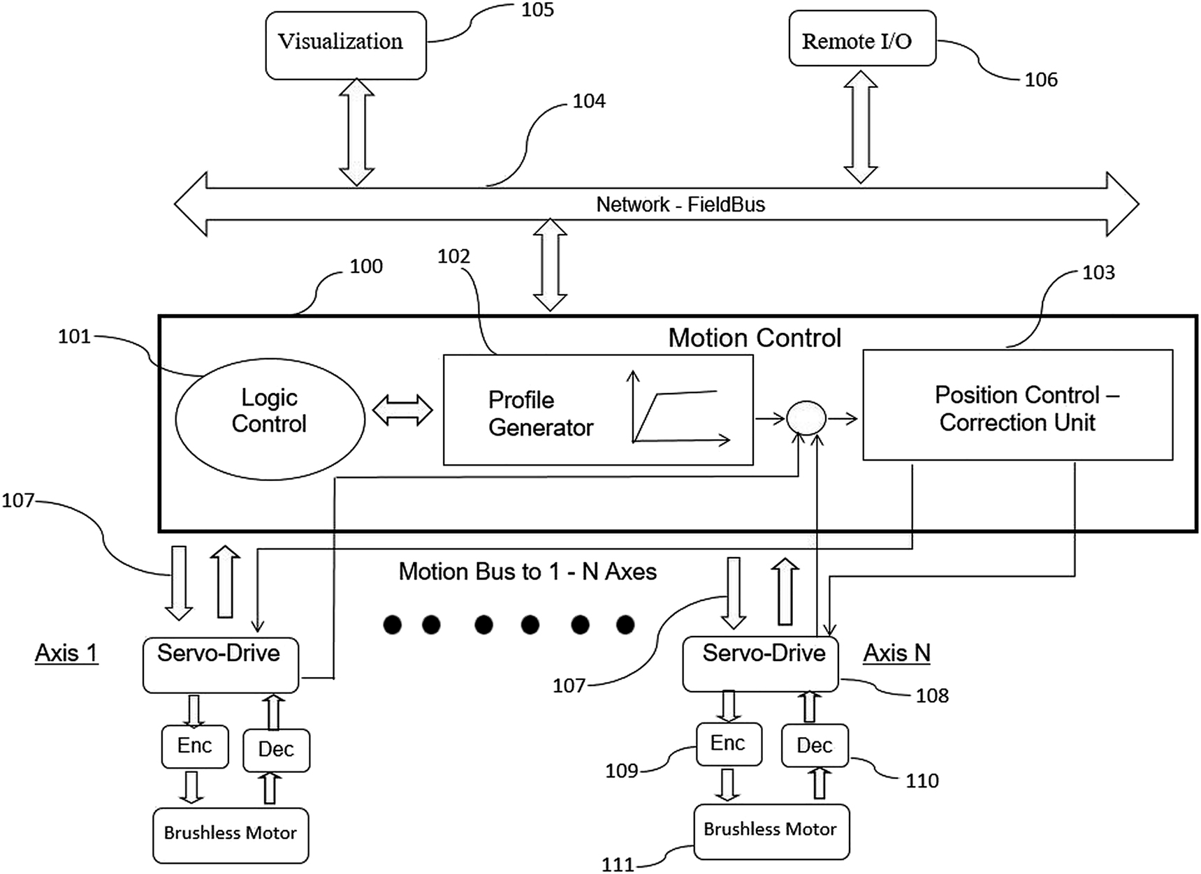
A detailed example relative to an architecture of a motion control system. The motion controller is represented, with his most important elements contained in it, plus the field-bus and the motion-bus to the N axes.

Furthermore, the motion control system is characterized by the following elements:

1. A drive or amplifier 108 for transforming the control signal from the motion controller into electric energy that is supplied to the actuator. Some newer “intelligent” drives can close the position and velocity loops internally, resulting in a very accurate control;

2. A prime mover or actuator such as a hydraulic pump, pneumatic cylinder, linear actuator, or electric motor 111 which transforms the electrical power into mechanical power. Mechanical components to transform the motion of the actuators into the desired motion, including gears, shafting, ball screw, belts, linkages, and linear or rotational bearings.

3. A position sensor (encoder 109 or resolver 110) for returning the position or the velocity of the actuator to the motion controller, to close the position or velocity control loops. That is in closed-loop systems.

4. Drivers plus prime mover plus position sensors together constitute the electric axis. Typically, a motion controller governs N different axes.

5. The motion bus 107, which is the physical and logical interface between the motion controller and the drives.

6. A field-bus 104, used to connect the elements of the motion controller system whose information can be transmitted in a nondeterministic way.

7. A display element 105 which is used as a control console and control system by the operator.

8. The input/outputs 106 necessary for the system, connected remotely to the controller via the field-bus.

2.2 Position control ring in a motion control system

A basic diagram of the control ring for the motion position in the closed-loop is shown in Figure 2.

Figure 2:

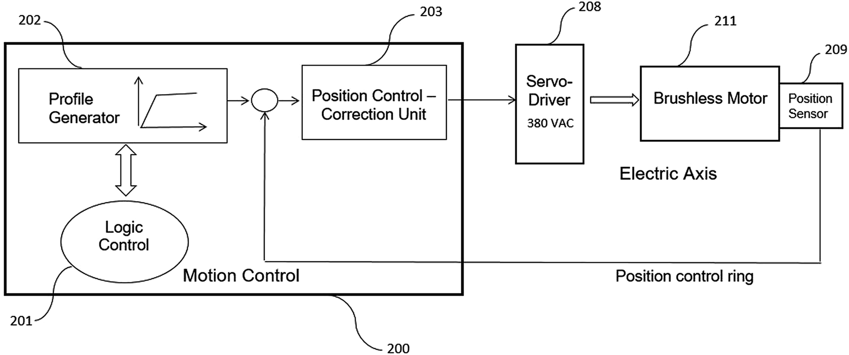
A diagram of the control ring for the position control system relative to a single “axis”. The same control rings are necessary for all the axes in the motion control system.

The system is based on a position control ring including the position controller 203, an electronic amplifier (driver) 208, an electric motor 211 and a position sensor 209.

Usually, the control rule is implemented using a trajectory generator 202 integrated into the motion controller 200 (as seen in Figure 1), just as the logic controller 201 and the position controller 203 are integrated therein.

The driver interposed between the motion controller and the electric motor is used for amplifying the control signal by supplying the electrical power necessary to power the motor in a controlled manner. Typically, the speed and torque control rings supplied by the motor are closed in the driver. In this case, the driver not only implements power amplification but also implements a complex law, dependent on the characteristics of the electric motor.

3.1 Detailed description

As previously described, the motion bus is a synchronous bus which is so-called because all the activities on that bus are synchronized using a clock. Therefore, as far as the deterministic part of the motion bus is concerned, it is fundamental that there is a synchronism as exact as possible between the communications that the master makes with the N slave axes.

The great advantage obtained with this new system compared to the existing motion controls is given by the fact that two optical generator units of entangled photons are introduced. That is made in order to perform a perfect synchronism between the N target positions transmitted from the master (virtual) to the N slaves, as well as in order to perform a perfect synchronism between the actual N positions transmitted by the position sensors to the master controller.

Referring to Figure 3, there is depicted, in a detailed way, a representation of this new system.

Figure 3:

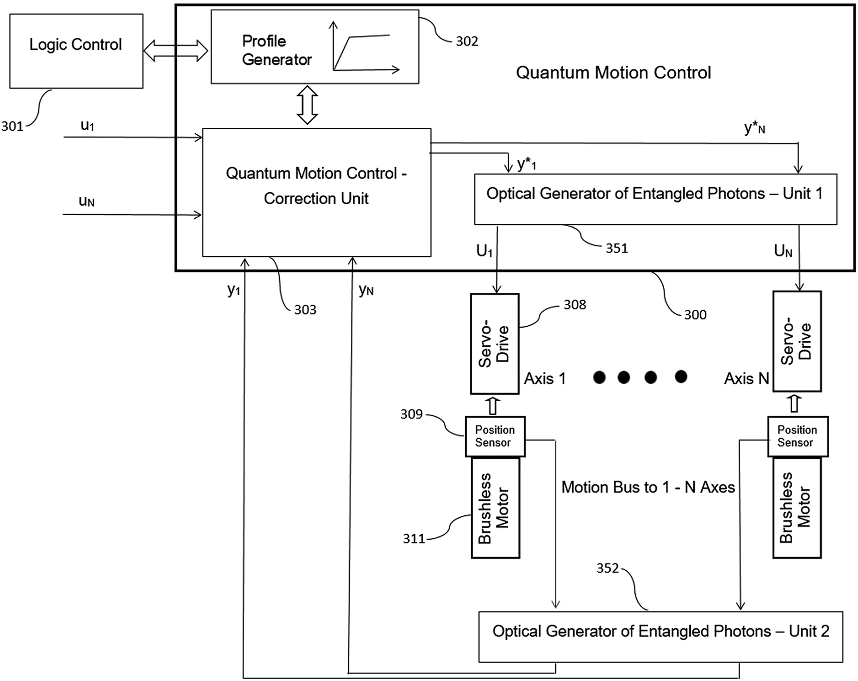
The novel architecture for the quantum motion control. A detailed diagram is depicted, with the representation of the main processes performed.

The central device 300 of the quantum motion control includes means for elaborating the necessary information in order to control the position of the N axes in movement. These means can consist of a correction unit 303 included in the quantum motion control device. Furthermore, these means can consist also of a profile generator 302 for generating a motion profile, having the task of generating a reference profile for the actuator movement. Again, the central device 300 of the quantum motion control includes also the means to generate optical information consisting of entangled photons. These means can consist, as in the realized example, of a first device 351 having the task of being an optical generator of entangled photons.

In turn, profile generator 302 includes means to exchange information with the logic control device 301. Concretely, the logic control device 301, as defined in this invention, can be a programmable logic controller. This device can be physically separated from the central device 300 of the quantum motion control or it can be included in the central device 300.

The above-mentioned information exchanged with the logic control device 301 is used for the following purposes:

1. Define when exchanging information with the N axes;

2. Define the management of the starts and stops of the N axes in order to start and finish the movements of the N axes;

3. Define the management of the malfunctions in the production activity controlled by the central device 300.

Considering the correction unit 303, it includes means for receiving the information u ₁, u ₂, …, u _N , which represent the set-point positions with respect to the N axes 1, 2, …, N. These means can be analog inputs or information arriving via field-bus from a control/command console.

Again, the correction unit 303 includes also means for receiving information y ₁, y ₂, …, y _N which represent the values of the actual positions relative to the N axes 1, 2, …, N. Such means can be, for example, inputs that represent optical information arriving from the device 352 described below.

Furthermore, the correction unit 303 also includes means for sending the information y 1 * , y 2 * , … , y N * , which represent the set-point positions with correction relative to the N axes 1, 2, …, N. The information y 1 * , y 2 * , … , y N * is defined “with correction” because they are the sum of the set-points u ₁, u ₂, …, u _N (arriving from a control unit) with the corrections generated in the correction unit 303 as a consequence of the actual positions y ₁, y ₂, …, y _N of the N axes 1, 2, …, N. These means can be, for example, analog or optical outputs that transmit the information to the first device 351 having the task of being an optical generator of entangled photons.

In turn, the 351 device includes means for receiving from the correction unit 303 the information y 1 * , y 2 * , … , y N * , which represent the set-point positions with correction relative to the N axes 1, 2, …, N. These means can be, for example, either analog inputs, or internal bus, or optical inputs used for receiving the information necessary to the here considered first device 351 that is used as an optical generator of entangled photons.

Again, the first device 351 having the task of being an optical generator of entangled photons includes also means for sending the information U ₁, U ₂, …, U _N to the N axes 1, 2, …, N. The information U ₁, U ₂, …, U _N represent the N set-point positions comprising the correction, after these set-points have been subjected, within the device 351, to the entanglement procedure between the photons carrying the information in them contained. These means used to send information U ₁, U ₂, …, U _N can be, for example, outputs that process the optical information obtained with the entanglement procedure in device 351.

Furthermore, the device 351 includes also means for implementing the photons entanglement procedure; those photons now carry the information given by the set-points with correction defined as y 1 * , y 2 * , … , y N * .

As regards the different ways in which we can practically realize the photons entanglement procedure in device 351, we refer to the different existing patents, mentioned in Section 1 of this work. In those patents, these modes of realization of different possible systems of entangled photons are described in detail.

Moreover, for the definition and the realization of the system for the transport of the information included in the entangled photons, we refer to the methods and systems described in the two articles published on Nature Photonics in 2016 and previously mentioned in Section 1 of this work.

It follows that the information U ₁, U ₂, …, U _N carried by the entangled photons reaches the servo-drives 308 and, then, the phenomenon of decoherence occurs. This, however, does not affect the information already conveyed and delivered to individual drivers via the optical path.

Corresponding to what was described previously about Figure 2, the position sensors 309 of the N axes 1, 2, …, N must send to the correction unit 303 the information given by the actual position of the corresponding axis. The position sensor is connected to the brushless motor 311 or, in any case, to the electric motor that produces the necessary energy to move the mechanical part of the axis.

Innovatively, in this method, the information given by the actual position of the single-axis is sent, in a preliminary step, to a second device 352 having the task of being an optical generator of entangled photons.

Device 352 includes means to send the information y ₁, y ₂, …, y _N to the correction unit 303 included in the central device 300 of the quantum motion control. The information y ₁, y ₂, …, y _N represents the N actual positions of the axes after this information has been subjected, inside the device 352, to the entangled photons generation process. These means used to send the information y ₁, y ₂, …, y _N can be, for example, outputs that process the optical information obtained with the entanglement procedure in the device 352.

Further, device 352 includes also means for implementing the photons entanglement process; those photons carry out the information given by the actual positions defined as y ₁, y ₂, …, y _N . As regards the different ways in which we can practically realize the photons entanglement process in device 352, we refer to the different existing patents, mentioned in Section 1 of this work. In those patents, these methods of realization of different possible entangled photons systems are described in detail.

Moreover, for the definition and the realization of the system for the transport of the information from the second entangled photons generation unit to the quantum motion control device, we refer to the methods and systems described in the two articles published on Nature Photonics in the 2016 and previously mentioned. In this way, the information given by the actual positions arrives in the correction unit into the quantum motion control device and the control loop is closed, as it should be in a motion control system with high performances.

3.2 Quantum nonlinear correction unit

In the present work, concerning Figure 4, the data processing which occurs internally to the correction unit 403, included in the central device of the quantum motion control, is schematized, following the guidelines developed in the U.S. patent application US 2013/0096698 A1 to S. Ulyanov.

Figure 4:

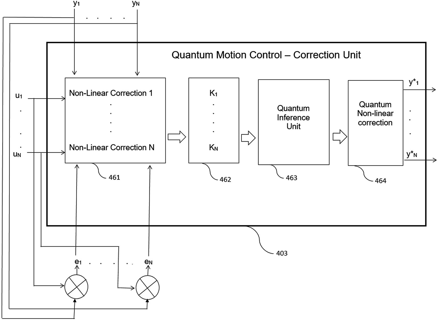
A quantum nonlinear correction unit, included in the quantum motion control device, is based on quantum inference. A block diagram, describing the subsequent steps for obtaining the correction to the set-position, is depicted.

As a consequence of that, in Figure 4, we show an example of a quantum nonlinear correction unit 403 included in the quantum motion control device and based on quantum inference. Referring to Figure 4, we define a block diagram describing the subsequent steps for obtaining the correction to the set-position, based on the actual position of the axes.

A self organizing controller is described, including a quantum inference unit 463 that can generate a set of robust control gains. The quantum inference unit 463 includes a quantum correlator configured for generating a plurality of quantum states based on a plurality of controller parameters and a correlation type.

Practically, the actual positions defined as y ₁, y ₂, …, y _N . are subtracted to the set-point positions u ₁, u ₂, …, u _N , relating, respectively, to the N axes 1, 2, …, N. That is made in order to obtain the differences e ₁, e ₂, …, e _N . These differences allow calculating the nonlinear corrections 461 for the set-points with correction defined as y 1 * , y 2 * , … , y N * .

Once the correction coefficients K ₁, K ₂, …, K _N are established in step 462 and after that the robustness of the control system has been implemented internally to the quantum inference unit 463, the quantum nonlinear corrections can be defined in step 464. In this way, the set-points with correction y 1 * , y 2 * , … , y N * are obtained.

3.3 Robust control in the quantum correction unit

In order to define the robustness of the proposed quantum motion control scheme we will refer to Figure 5 that shows, in a detailed way, the feedback loop that was schematized in a general form in the previous subsection. That is implemented internally to the quantum inference unit.

Figure 5:

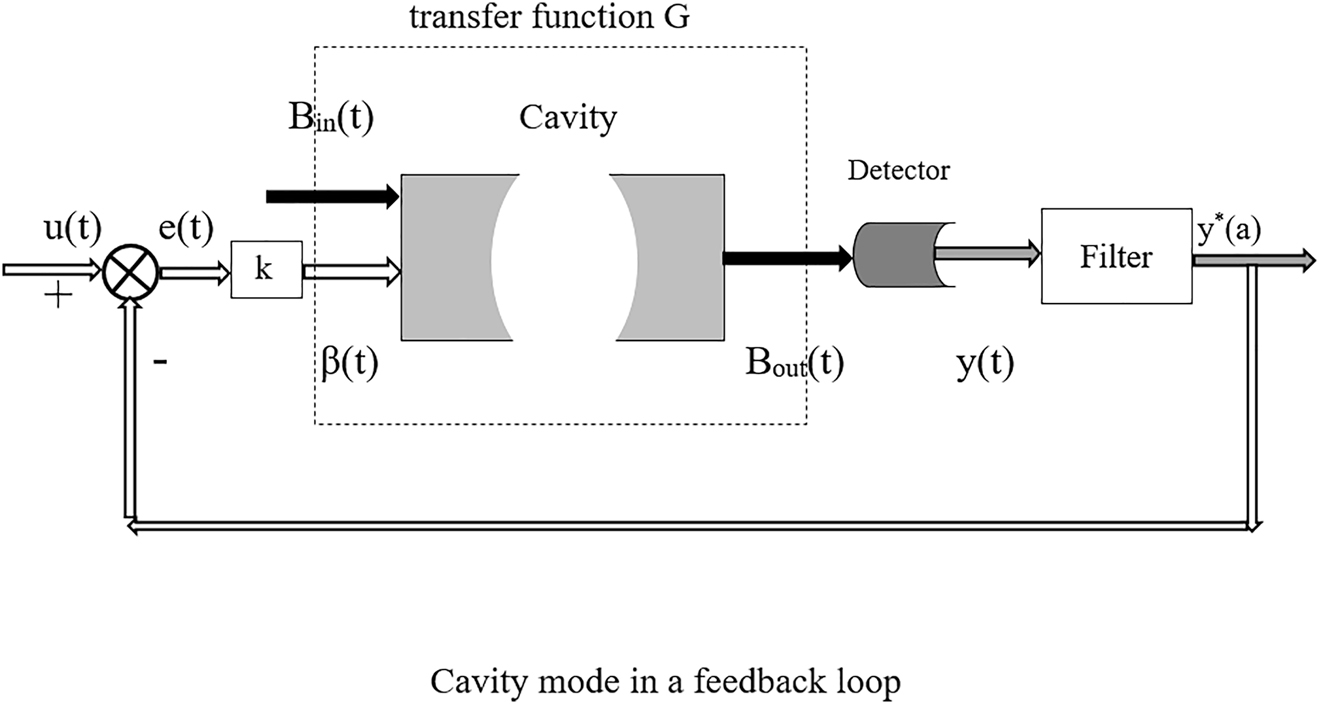
The feedback loop going through the cavity mode. It is highlighted the transfer function G. That is implemented internally to the quantum inference unit.

We refer in this section to only an axis. The same loop has to be considered for each axis in the quantum motion controller.

In recent work, Gough [25] defined a controlled quantum stochastic dynamical model, defined as a cavity mode, with a PID controller acting on the filtered estimate output y. We will base on that work for defining the robust control of the quantum motion controller. Therefore, the theory that is described below is basically defined on what is described in the work of Gough [25].

For now, we will focus on the linear solution. The robustness of the nonlinear solution will be the subject of a further study which is currently under preparation.

In Figure 5 we will use white double-lined arrows to denote classical signals in feedback block diagrams and single-line arrows (gray or black) for quantum signals.

The most used control algorithm in classical feedback applications are the PID controllers, with PI action used as most common form. For them, we have the input–output relation:

where the constants k _P , k _I , k _D are the PID gains, respectively. The associated transfer function is K(s) = k _P + s ⁻¹ k _I + sk _D .

The goal of filtering theory is to make an optimal estimate of the state of a system under conditions where the system may have noisy dynamics, and where may have only partial information which also is subject to observation noise.

In order to go deep into the definition of the correction unit in the quantum motion controller, schematized in Figure 4, we consider the diagram in Figure 5, where we represent the realized closed-loop for obtaining the single set-points with correction y i * .

Considering a system that is supposed to evolve according to linear but noisy dynamics of the form

where the x _k are the state at time k, the u _k are control variables, and w _k are errors. Our knowledge is based on measurements that explain only partial information about the state and also present noise. Specifically, the measure y _k at time k was

The random variables w _k , v _k are the dynamical noise and measurement noise and follow a Gaussian profile.

The Kalman filter is a recursive estimation scheme, requiring minimal storage of information, valid for Gaussian models. Considering the best estimation x ̂ k − 1 , we can predict x ̃ k = A x ̂ k − 1 + B u k . Therefore, we can predict that the next observation should be y ̃ k = H x ̃ k . That will be fundamental is the residual error which is the difference between the observed value of y _k and the expected value, y ̃ k = H x ̃ k . This is defined as the innovations process:

If this error is zero, then the prediction is exact, and we can use the prediction x _k as an estimation for the state at time k. Otherwise, we can apply in a recursive way the Kalman filter, setting x ̂ k = x ̃ k + H P ̃ k I k , being the prediction error P ̃ k = Var ( x k − x ̃ k ) .

The theory of quantum filtering was developed by Belavkin [26], and represents the continuation of the works of Kalman, Stratanovich, Zakai, etc. Qubits pass through a cavity (Figure 5) one by one. We measure the outgoing qubits one-by-one. The measurement bit y _k is sent into a filter that estimates the state of the cavity mode, and then the instruction is sent to the actuator in order to have the control of the mode.

In our quantum model, based on the traditional Kalman filter, we monitor a cavity model. We will refer to the notation used in [27, 28] and to the development defined in those works relative to the quantum filters. We denote the mode by a. The transfer function G for a quantum system driven by boson fields is defined given the SLH-coefficients component the transfer function G. We consider the S, L, H components of the triple operator (the transfer function G) which represents the coupling between an individual node of a network (in this case atoms in a cavity), and the interacting quantum field. These S, L, H coefficients are obtained in the following way:

where β ^[[Z]](t) is an unspecified complex-valued adapted process controlled by Z. Z is defined as Z(t) = B _in(t) + B _in(t)* and Y is given by Y(t) = B _out(t) + B _out(t)* (see Figure 5). This in the hypothesis of quadrature between the measurements. For more details relatively to the SLH formalism see [29].

The Heisemberg–Langevin equation satisfied by a t = j t [ [ Y ] ] ( a ) is now

This is the output form of the control process. If we measure the situation in which θ = 0, then the Belavkin–Lalman output filter (see [25]) for a ̃ t = π t ‖ Y ‖ ( a ) will be

where the innovation is d I ( t ) = d Y ( t ) − γ ( a ̂ t + a ̂ t * ) d t . The covariances W ( t ) and V ( t ) are deterministic function satisfying the coupled deterministic ordinary differential equations (ODEs):

Reverting back the signal to the input (see Figure 5) and starting by Eq. (6), we obtain for the feedback signal the corresponding equation relative to the input filter (see [25]):

where d J ( t ) = d Z ( t ) − γ ω ̄ t [ [ Z ] ] ( a ) + ω ̄ t [ [ Z ] ] ( a ) * d t .

Referring to Figure 5, closing the feedback loop we take:

In Eq. (11) we included a reference signal u(t) and computed the error e ( t ) = u ( t ) − ω ̄ t [ [ Z ] ] ( a ) . This error is multiplied for a constant gain k before obtaining the controlling process β t [ [ Z ] ] . Returning to the output, from Eq. (11) we have:

When k → ∞, we can expect the cavity mode to track the reference signal u(t). More generally, we consider a proportional-integral (PI) controller having the output given by Eq. (1) without the derivative term. We will denote the Laplace transform of a function f = f(t) by f [ s ] = ∫ 0 ∞ e − s t e ( t ) d t . We use square brackets for the transform parameter. β[s] = K(s)e[s] where the controller transfer function is K ( s ) = k P + k I 1 s . We can compute that the analogue of Eq. (12) is

where the open-loop function transfer for the system mode is G ( s ) = s + γ 2 + i ω − 1 and the closed loop transfer function is H = GK/(1 + GK). The term N(s) is the noise due to the innovations and it given by:

For the PI problem, the closed-loop transfer function is:

For the PID problem, the closed-loop transfer function should be:

However, there is a problem. The error is the difference between the reference signal and the filtered estimate ω ̄ t [ [ Z ] ] ( a ) , but the latter is a stochastic process and so it is not differentiable in the traditional way. We need to use the quantum Ito calculus for a stochastic process. For more information relative to the detailed calculation of the terms of H _PID see ([25]).

3.4 Comparison with traditional motion control: improving performance for the jitter compensation

In order to consider a comparison between the performances of traditional motion control and the proposed quantum motion control, we will focus our interest on the jitter compensation.

Leveraging the ideas from [30], the periodic task model considers a digital control system set. It is implemented as a periodic task set T _i ∈ T ₁, T ₂, …, T _n . T _i corresponds to an individual control task, and it has an infinity job set J _i,j ∈ J _i,1, J _i,2, …. The job J _i,j is an instantiation of a control task T _i .

Figure 6 depicts a timing diagram of control task T _i for four consecutive jobs J _i,k−2 to J _i,k+1.

Figure 6:

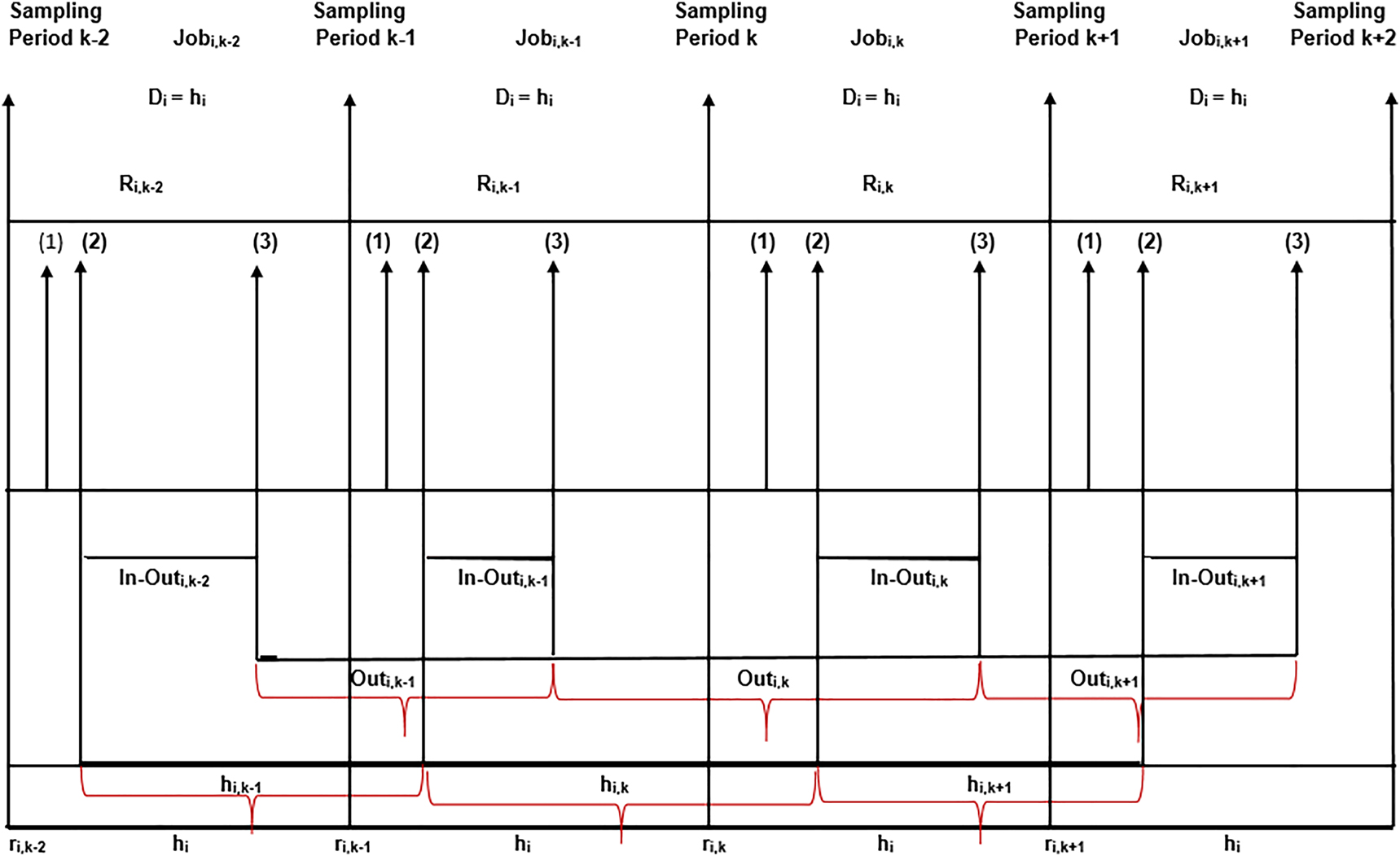
A timing diagram of control task T _i for four consecutive jobs J _i,k−2 to J _i,k+1.

The relative deadline D _i of each control task T _i is equal to its sampling period h _i . Furthermore, the relative deadline D _i for the job J _i,j is measured from its release time r _i,j . The response time R _i,j is the necessary time until the control law is output relatively to the job J _i,j . InOut _i,j is the time to output the control law by the digital to analog converter (DAC) relative to the start of sampling the inputs for job J _i,j (time between events (2) and (3) in Figure 6). Out _i,j is the time between outputting the control law (event (3) in Figure 6) for jobs J _i,j−1 and J _i,j . h _i,j is the time between sampling points (event (2) in Figure 6) for jobs J _i,j−1 and J _i,j . h _i,j is defined as the “sampling interval” for job J _i,j . In fact, in a realistic implementation of a motion controller, all three events (1), (2) and (3) are delayed from their original timing instant. For example, event (3) is delayed by InOut _i,j relative to event (2).

Because a motion controller has periodic events, the timing of these events can vary from one period to another. This phenomenon is defined as “Jitter”. We will consider four jitter terms:

1. “Input–Output Jitter”: the variation of InOut _i,j for T _i .

2. “Output Jitter”: the variation of Out _i,j for T _i .

3. “Sampling Jitter”: the variation of the “sampling interval” h _i,j for T _i .

4. “Synchronization Jitter”: the variation time ΔT _i between the different command signals that, for each T _i , the motion controller send to the 1…N different controlled axes. In other words, this is the jitter which is introduced when considering N axes that must be coordinated simultaneously by the motion controller.

As we can note in Figure 6, the notion of sampling interval is not the same as the sampling period in the context of executing multiple control tasks on the same processor.

In fact, the sampling period is always equal to h _i for the task T _i . On the other hand, the sampling interval for job J _i,j at times can be 0 < h _i,j < h _i or at times can be h _i < h _i,j < 2h _i . In other words, that is fundamental in the definition of the jitter of a motion controller and therefore in the precision relative to a positioning command for a controlled axis.

Analyzing the characteristics described in the previous sections relative to the quantum motion controller, and defining the performance improvements compared to the traditional motion controllers, we can deduce that the first three types of jitter are not modified with the introduction of a quantum motion controller.

Both the “Input–Output Jitter”, the “Output Jitter” and the “Sampling Jitter” are not affected by the new configuration of the motion controller. On the other hand, the case of the “Synchronization Jitter” is different. As described in the Introduction, considering the deterministic part of the communication cycle, the motion controller will send the target positions to the axes in a synchronized manner and will receive the actual positions in an equally synchronous manner from the axes themselves. It is therefore essential that there is a synchronism as exact as possible between the communications that the master makes with the N slave axes. Even a 1 micros “Synchronization Jitter” can generate accumulative errors in the final element of the kinematic chain that is the prime mover.

In the present work, we defined a system where the data are exchanged between the controller master and the different slave drives taking advantage of the quantum system properties. Exactly, we use the entanglement property of the photons generated in the optical units for having a perfect synchronization among the N target positions sent, in the same instant t, to the N slave drives and the same perfect synchronization among the N actual positions received, subsequently, from the N slave drives.

This is the considerable improvement obtained in the solution presented in this work: The achievement to eliminate the “Synchronization Jitter” between the signal transmitted and received by the N slave axes.

3.5 Best mode for carrying out the quantum motion control

The logical flow of information that, in practice, occurs when this method is carried out, it is the following.

Considering the case of a packaging machine, the required data, both for the setting of the machine and for the setting of the various possible formats of the products that must be packaged, are inserted through a display unit that acts as a supervision unit.

Simultaneously one or more operators, using command keyboards, send either the start command or the stop in ramp command or the emergency stop command, necessary to command the movement of the axes of the packaging machine. These data, from the display and the command consoles, are sent, typically via a field-bus, both to the logic control device (typically, a Plc that can also be integrated into the motion control device) and to the unit that generates the motion profiles internally to the motion control device.

At this point, based on the machine commands received from the motion control device, the next step consists of the definition, inside the unit that generates the motion profiles, of the motion profiles related to the machine axes. These motion profiles will generate electronic cams that will be different depending on the type of “axes” that must command (linear, rotating, epicyclical, etc.), and on the command received by the operator (run, ramp stop, emergency stop, etc.).

The next logical step is obtained in the quantum nonlinear correction unit, where the actual positions of the “axes” are subtracted to the respective set-point positions: that is made in order to obtain the error differences. These differences allow for calculating the nonlinear corrections for the set-points with correction.

Once the correction coefficients are obtained, and after that the robustness of the control system has been increased using the quantum inference unit, the nonlinear corrections are defined in this step.

Now, the nonlinear corrections are sent from the quantum nonlinear correction unit to the first device having the task of being an optical generator of entangled photons.

In a first possible representation, the information relative to the N axes, which symbolize the set-point positions with correction, can be sent using an internal bus or using an analog connection. Corresponding, also the fundamental information of the clock used for synchronizing the information representing the set-point positions to send to the N axes, is sent to the first optical generator of entangled photons.

In this kind of representation, the first device having the task of being an optical generator of entangled photons simply receive the information representing the set-point positions with correction relative to the N axes and sends directly them to the N axes.

Besides, always considering this first possible representation and using the U.S. patent application US 8242435 B2 to Shin Arahira, the entangled photons, symbolizing the clock used for synchronizing the set positions for the N axes, are obtained starting from an excitation light (resulting from the clock signal). It is split into two components with mutually orthogonal polarization. In the unit, as described in the considered patent, at the end of the process, idler photons and signal entangled photons are obtained. The second represents the clock signals that are sent to the N axes.

On the other hand, in a second possible representation, the signal entangled photons obtained, at the end of the described process, also contain the information representing the set-point positions with correction relative to the N axes and not only the clock used for synchronizing the information representing the same set-point positions.

As the next step, we consider the system for the transport of the information included in the entangled photons. Regarding that, we refer to the methods and systems described in the two articles published on Nature Photonics in 2016 and previously mentioned.

Following what is described in those articles, we can define an optical-fiber-based quantum network. This network is robust against noise in the real environment with active stabilization strategies, and this property allows for realizing quantum teleportation with all the ingredients simultaneously.

Therefore, it follows that the information carried by the entangled photons reaches the servo-drives via the optical path.

After that, in the logical flow of information, the position sensors of the N axes send the information given by the actual positions of the single axes to a second device having the task of being an optical generator of entangled photons.

This device works in the same way and with the same characteristics of the first optical generator of entangled photons and produces, at the end of his internal process, the “entangled” information given by the actual positions of the single axes. These data are sent, using the system for the transport of the entangled photons previously described, to the correction unit in the quantum motion control device.

The control loop is thus closed and the system can process, in a subsequent cycle, the information coming from the command data entry systems.

References

[1] R. P. L. Caporali, “Method and Device to control in open-loop the sway of pay-load for Slewing Cranes,” Patent EP 2896590, Jul. 22, 2015. Available at: Google Patents.Suche in Google Scholar
[2] R. P. L. Caporali, “Iterative method for controlling with a command profile the sway of a payload for gantry and overhead traveling cranes,” Int. J. Innov. Comput. Inf. Control, vol. 14, no. 3, pp. 1095–1112, 2018, Available at: http://www.ijicic.org/ijicic-140401.pdf.Suche in Google Scholar
[3] L. Pengfei, H. Yuping, W. Yanbo, Z. Quing, and Y. Zelin, “Design of multi-axis motion control and drive system based on internet,” in Presented at the 22nd Int. Conf. on Electrical Machines and Systems (ICEMS), Harbin, China, 2019, Available at: https://ieeexplore.ieee.org/document/8921848.10.1109/ICEMS.2019.8921848Suche in Google Scholar
[4] D. Zhao, J. Gui, J. Yang, S. Li, and W. Cao, “Sliding mode control with extended state observer for multi-axis motion control system,” in Presented at the 2019 Chinese Control Conference (CCC), Guangzhou, China, 2019, Available at: https://ieeexplore.ieee.org/document/8865713.10.23919/ChiCC.2019.8865713Suche in Google Scholar
[5] Z. Zeng, Y. He, Y. Hu, et al.., “Fine tuning development software for high precision and Multi-Axis Motion Control System,” in Presented at the 18th International Conference on Electronic Packaging Technology (ICEPT), Harbin, China, 2017, Available at: https://ieeexplore.ieee.org/document/8046591.10.1109/ICEPT.2017.8046591Suche in Google Scholar
[6] S. A. Berestova, N. E. Misyura, and E. A. Mityushov, “Mechanics of smooth coordinated motion of multi-Axis mechatronic device,” in Presented at the 2019 International Russian Automation Conference (RusAutoCon), Sochi, Russia, 2019, Available at: https://ieeexplore.ieee.org/document/8867730.10.1109/RUSAUTOCON.2019.8867730Suche in Google Scholar
[7] C. Hu, T. Ou, H. Chang, Z. Yu, and L. Zhu, “Deep GRU neural-network prediction and feedforward compensation for precision multi-Axis motion control systems,” IEEE ASME Trans. Mechatron., vol. 25, pp. 1377–1388, 2020. https://doi.org/10.1109/TMECH.2020.2975343.Suche in Google Scholar
[8] G. Zhong, Z. Shao, H. Deng, and J. Ren, “Precise position synchronous control for multi-Axis servo systems,” IEEE Trans. Ind. Electron., vol. 64, pp. 3707–3717, 2017. https://doi.org/10.1109/TIE.2017.2652343.Suche in Google Scholar
[9] M. Tiapkin, D. Elenskiy, and A. Balkovoi, “Observer-based control system design of high performance motion system with parallel kinematics,” in Presented at the 2018 X International Conference on Electrical Power Drive Systems (ICEPDS), Novocherkassk, Russia, 2018, Available at: https://ieeexplore.ieee.org/document/8571480.10.1109/ICEPDS.2018.8571480Suche in Google Scholar
[10] J. Sorensen, D. O’Sullivan, and C. Aaen, “Synchronization of multi-Axis motion control over real-time networks,” in Presented at the 2018; International Exhibition and Conference for Power Electronics, Intelligent Motion, Nuremberg, Germany, Renewable Energy and Energy Management, 2018, Available at: https://ieeexplore.ieee.org/document/8402996.Suche in Google Scholar
[11] C. Ma, X. Zhang, Y. Yan, and T. Shi, “Predictive contour control for multi-axis motion system with unified model,” in Presented at the 2019 22nd International Conference on Electrical Machines and Systems (ICEMS), Harbin, China, 2019, Available at: https://ieeexplore.ieee.org/document/8921467.10.1109/ICEMS.2019.8921467Suche in Google Scholar
[12] Z. Liu and J. Yang, “Sliding-mode control-based adaptive PID control with compensation controller for motion synchronization of dual servo system,” in Presented at the 2017 36th Chinese Control Conference (CCC), Dalian, China, 2017, Available at: https://ieeexplore.ieee.org/document/8028133.10.23919/ChiCC.2017.8028133Suche in Google Scholar
[13] E. Fertig, “Packaging machine and method for controlling a packaging machine,” Patent EP 1431187 A3, Jun. 23, 2004. Available: Google Patents.Suche in Google Scholar
[14] S. Konze, P. Theissen, and L. Merten, “Method for controlling a packaging machine and a Packaging machine,” Patent US 2017/0001744 A1, Jan. 5, 2017. Available: Google Patents.Suche in Google Scholar
[15] L. Biagiotti, C. Melchiorri, M. Pilati, G. Mazzucchetti, G. Collepalumbo, and P. Ragazzini, “Integration of robotic systems in a packaging machine: a tool for design and simulation of efficient motion trajectories,” in Presented at the 2013 IEEE 18th Conference on Emerging Technologies Factory and Automation (ETFA), Cagliari, Italy, 2013, Available at: https://ieeexplore.ieee.org/document/6648125.10.1109/ETFA.2013.6648125Suche in Google Scholar
[16] S. Ulyanov, G. Rizzotto, I. Kurawaki, et al.., “Method and Hardware Architecture for controlling a process or for processing data based on a quantum soft computing,” Patent WO/2001/067186, Sep. 13, 2001. Available at: Google Patents.Suche in Google Scholar
[17] G. Kanter and S. Wang, “System and method for entangled photons generation and measurement,” Patent US 2010/0309469 A1, Feb. 26, 2010. Available at: Google Patents.Suche in Google Scholar
[18] K. Edamatsu, R. Shimizu, and S. Nagano, “Non-degenerate polarization-entangled photon pair generation device and non-degenerate polarization-entangled photon pair generation method,” Patent US 2012/8173982 B2, May 26, 2012. Available at: Google Patents.Suche in Google Scholar
[19] P. Senellart and A. Dousse, “Polarization-entangled photon pair source and method for the manufacture thereof,” Patent EP 2526459 A1, Nov. 28, 2012. Available at: Google Patents.Suche in Google Scholar
[20] S. Arahira, “Quantum entangled photon pair generating device and method,” Patent US 2012/0051740A1, Mar. 01, 2012. Available at: Google Patents.Suche in Google Scholar
[21] S. Qi-Chao, M. Ya-Li, C. Si-Jing, et al.., “Quantum teleportation with independent sources and prior entanglement distribution over a network,” Nat. Photonics, vol. 10, pp. 671–675, 2016, Available at: https://www.nature.com/articles/nphoton.2016.179.10.1038/nphoton.2016.179Suche in Google Scholar
[22] R. Valivarthi, M. Grimau Puigibert, Z. Quiang, et al.., “Quantum teleportation across a metropolitan fibre network,” Nat. Photonics, vol. 10, pp. 676–680, 2016. https://doi.org/10.1038/nphoton.2016.180.Suche in Google Scholar
[23] M. Brodsky and M. Feuer, “Architecture for reconfigurable quantum key distribution networks based on entangled photons directed by a wavelength selective switch,” Patent US 2012/8311221 B2, Nov. 13, 2012. Available at: Google Patents.Suche in Google Scholar
[24] S. Ulyanov, “Self-organizing quantum robust control methods and systems for situations with uncertainty and risk,” Patent US 2014/8788450 B2, Jul. 22, 2014. Available at: Google Patents.Suche in Google Scholar
[25] J. E. Gough, “A quantum Kalman filter-based PID controller,” Open Syst. Inf. Dynam., vol. 27, no. 3, 2020. https://doi.org/10.1142/s1230161220500146.Suche in Google Scholar
[26] V. P. Belavkin, “Non-Demolition measurements, nonlinear filtering and dynamic programming of quantum stochastic processes,” Lect. Notes Contr. Inf. Sci., vol. 121, pp. 245–265, 1989.10.1007/BFb0041197Suche in Google Scholar
[27] L. Bouten and R. van Handel, “On the separation principle of quantum control,” in Quantum Stochastic and Information: Statistics, Filtering and Control, Singapore, World Scientic Publishing Co Pte Ltd, 2008.10.1142/9789812832962_0010Suche in Google Scholar
[28] L. Bouten, R. van Handel, and M. R. James, “An introduction to quantum leering,” SIAM J. Contr. Optim., vol. 46, p. 2199, 2007. https://doi.org/10.1137/060651239.Suche in Google Scholar
[29] J. Combes, J. Kerckhoff, and M. Sarovar, “The SLH framework for modeling quantum input-output networks,” Adv. Phys. X, vol. 2, no. 3, pp. 784–888, 2017. https://doi.org/10.1080/23746149.2017.1343097.Suche in Google Scholar
[30] J. W. S. Liu, Real-Time Systems, NJ, Prentice-Hall, 2000.Suche in Google Scholar
© 2021 the author(s), published by De Gruyter, Berlin/Boston
This work is licensed under the Creative Commons Attribution 4.0 International License.
Artikel in diesem Heft
- Frontmatter
- Original Research Articles
- Modeling and assessment of the flow and air pollutants dispersion during chemical reactions from power plant activities
- Stochastic dynamics of dielectric elastomer balloon with viscoelasticity under pressure disturbance
- Unsteady MHD natural convection flow of a nanofluid inside an inclined square cavity containing a heated circular obstacle
- Fractional-order generalized Legendre wavelets and their applications to fractional Riccati differential equations
- Battery discharging model on fractal time sets
- Adaptive neural network control of second-order underactuated systems with prescribed performance constraints
- Optimal control for dengue eradication program under the media awareness effect
- Shifted Legendre spectral collocation technique for solving stochastic Volterra–Fredholm integral equations
- Modeling and simulations of a Zika virus as a mosquito-borne transmitted disease with environmental fluctuations
- Mathematical analysis of the impact of vaccination and poor sanitation on the dynamics of poliomyelitis
- Anti-sway method for reducing vibrations on a tower crane structure
-
Stable soliton solutions to the time fractional evolution equations in mathematical physics via the new generalized
- Convergence analysis of online learning algorithm with two-stage step size
- An estimative (warning) model for recognition of pandemic nature of virus infections
- Interaction among a lump, periodic waves, and kink solutions to the KP-BBM equation
- Global exponential stability of periodic solution of delayed discontinuous Cohen–Grossberg neural networks and its applications
- An efficient class of fourth-order derivative-free method for multiple-roots
- Numerical modeling of thermal influence to pollutant dispersion and dynamics of particles motion with various sizes in idealized street canyon
- Construction of breather solutions and N-soliton for the higher order dimensional Caudrey–Dodd–Gibbon–Sawada–Kotera equation arising from wave patterns
- Delay-dependent robust stability analysis of uncertain fractional-order neutral systems with distributed delays and nonlinear perturbations subject to input saturation
- Construction of complexiton-type solutions using bilinear form of Hirota-type
- Inverse estimation of time-varying heat transfer coefficients for a hollow cylinder by using self-learning particle swarm optimization
- Infinite line of equilibriums in a novel fractional map with coexisting infinitely many attractors and initial offset boosting
- Lump solutions to a generalized nonlinear PDE with four fourth-order terms