
Price Stickiness, Input–Output Linkages, and Monetary Policy Transmission in Korea
-
Seungyoon Lee


Abstract
This study investigates the industry effects of monetary policy in Korea by analyzing the role of sectoral heterogeneity regarding price stickiness and inter-industry relations. I extend a standard sticky-price Dynamic Stochastic General Equilibrium (DSGE) model into a model with heterogeneous production sectors, where each industry sector is allowed to have distinct price stickiness and inter-industry production linkages. Input–Output matrices are utilized to construct the inter-industry linkages, which reflect the use of final products from other sectors as material inputs or investment goods. Sectoral price stickiness and other model parameters are estimated using a Bayesian approach. From the estimated model, the asymmetric impact of monetary policy across sectors is investigated. Simulated impulse responses suggest that sectoral variables exhibit clear comovements in response to monetary policy shocks while the magnitudes of the responses differ considerably across sectors, which can be attributed to the differences in price rigidities and production linkages. Compared to the results from a standard single-sector model, the output response is more pronounced, while the inflation response diminishes. The results indicate that ignoring sectoral heterogeneities could bias estimates of monetary policy effects.
1 Introduction
This study constructs a New Keynesian Dynamic Stochastic General Equilibrium (NK-DSGE) model incorporating multiple heterogeneous production sectors, and estimates the model through a Bayesian method using Korean data. Based on the estimated model, the asymmetric transmission of monetary policy across industry sectors is investigated. Central banks conduct monetary policy by adjusting policy rates, which are interest rates applied to short-term interbank transactions, to influence real interest rates and aggregate demand. The transmission of the monetary policy implementation can vary quantitatively across industry sectors depending on the characteristics of production sectors. In this study, I focus on two features. The first is possible differences in price-setting behavior. Within the New Keynesian framework, the impact of monetary policy on output is expected to be more pronounced if firms face difficulties in adjusting the prices of their goods and services and instead accommodate changes in aggregate demand by altering production quantities. This well-known transmission mechanism of monetary policy in a New Keynesian framework is naturally extended to a multisector model. That is, any differences in the extent of sectoral price rigidity would generate asymmetric effects of monetary policy on outputs across sectors. The second is inter-industry production linkages. Each industry uses final products produced by other sectors in its production process as production factors, such as material inputs and investment goods, and at the same time, some of their final products are used as production factors in other sectors’ production. Through this inter-industry linkage, production in one sector transmits to the production of other sectors. The extent to which each industry affects (and is affected by) other sectors’ production through the network could be another important source of asymmetric impacts of monetary policy. The larger the portion of a sector’s products used as production factors, the greater the sector’s output response, as overall demand for its final products from other sectors increases and thus amplifies the initial impact of the monetary expansion on output.
The model comprises infinitely lived identical households, distinct production sectors, and a monetary authority. Within each sector, two types of entrepreneurs exist: wholesale goods producers and retailers. The former produces wholesale products using production factors either produced by firms in its own sector or sourced from firms in other sectors. The latter produces differentiated goods using wholesale products under the assumption of monopolistic competition and implicit costs of nominal price adjustment. The assumption that only a fraction of retailers can adjust their prices in each period introduces price stickiness à la Calvo style. Monetary policy is implemented such that the central bank adjusts its nominal policy rate to stabilize the inflation gap and the output gap according to a typical Taylor rule. The key distinction from a standard NK-DSGE model is the presence of multiple heterogeneous production sectors and inter-industry linkage effects among them.
At the stage of grafting the theoretical model onto a real economy, I focus on six broad sectors in Korea: Agriculture, Mining, Manufacturing, Utilities, Construction, and Services. Inter-industry dependencies regarding the use of material inputs and investment goods in production are established using Input–Output tables and the National Accounts in Korea. Each of the Cobb-Douglas production functions of the six sectors is estimated separately using annual data on nominal expenditures, such as employee compensation and intermediate consumption, as well as the level of capital stock, under the assumption of constant returns to scale (CRTS) with three production factors (labor, capital stock, and material inputs). A Bayesian estimation approach is adopted to estimate the rest of the model parameters, including those regarding sectoral price rigidities and the monetary policy rule, using aggregate and sectoral quarterly data.
I find that substantial sectoral heterogeneities exist in terms of production technology, inter-industry relations, and price rigidities. Looking at the estimated output elasticities or the share of factor incomes in the production functions, the parameter for material inputs is found to be the largest of the three production factors across all six industries, ranging from 0.39 (Services) to 0.76 (Manufacturing). This indicates that it is an important factor in the production process that should not be ignored, and at the same time, that there exists a significant heterogeneity in factor elasticities. By analyzing the Input–Output matrix for material inputs, I find that self-sufficiency rates (the share of material inputs sourced within the same sector) exceed 0.6 in Manufacturing and Services but are near zero in Mining and Construction. In other words, the dependence on material inputs produced in other sectors is at least 0.3 and close to 1 at most, which reveals that production linkages in the overall economy are substantial, and at the same time, the degree of inter-industry dependence differs markedly across sectors. From the Bayesian estimation results, I find that there exists considerable price rigidity for the whole economy, with varying degrees of stickiness across sectors. To be specific, prices in the entire economy are estimated to remain unchanged for an average of 3.71 quarters, and prices in Services are the most rigid (5.38 quarters), followed by Utilities (3.36 quarters), Mining (2.74 quarters), and Manufacturing (2.23 quarters). Prices are found to be relatively flexible in Construction (1.84 quarters) and Agriculture (1.47 quarters).
I then simulate the impulse responses of sectoral and aggregate variables in response to a monetary policy easing shock using the estimated model. The results indicate that sectoral variables show positive correlations in their responses to monetary policy shocks, while the magnitudes of the responses differ markedly, as expected. Price rigidities and production linkages are found to play an important role in generating asymmetric sectoral responses. Specifically, sectoral output responses are proportional to the degree of price stickiness and the use of final products as material inputs or investment goods. Firms in sectors with stickier price adjustments are more likely to accommodate increased demand by raising output, and this leads to larger output responses. In sectors where their final products are extensively used in the production process, output expands further to meet increased demand for production factors. To investigate the relative importance of the two aspects in each industry, I simulate the responses to monetary policy shocks with one of the two channels deactivated. From these counterfactual analyses, I infer that the large responses in Mining and Construction output stem from the fact that their products are used mainly as material inputs and investment goods, respectively. The responses of Manufacturing and Utilities reflect relatively higher proportions of their final products being demanded as production factors. Despite the most rigid price-setting behavior, Services show relatively subdued responses due to the relatively small fraction of its products being used as production factors. The output expansion in Agriculture is limited due to flexible prices and less extensive use of its final products as production factors. Compared to the responses from a standard single-sector DSGE model, the aggregate output response is more significant, while the inflation response is smaller. The simulation results indicate that the quantitative estimates of monetary policy transmission for both aggregate and sectoral variables could be biased if sectoral heterogeneities and production linkages are not considered.
This study builds on the literature investigating production networks and its macroeconomic implications in multisector production models (Horvath 1998, 2000, Acemoglu et al. 2012, 2016, Petrella et al. 2019, Ferrante et al. 2023). Several studies are closely related to this study by examining monetary policy transmission in multisector economies (Carvalho 2006, Nakamura and Steinsson 2010, Bouakez et al. 2009, 2011, 2014, Pasten et al. 2020, Ghassibe 2021, La’O and Tahbaz-Salehi 2022). The production network in this study is closest to that in Bouakez et al. (2009), which investigates heterogeneous monetary policy transmission across U.S. industries but differs in the settings of price rigidity and monetary policy rules. Empirical evidence shows positively correlated but quantitatively heterogeneous output responses across industries to monetary policy shocks in studies examining the U.S., Europe, and Korea (Barth et al. 2001, Peersman and Smets 2005, Dedola and Lippi 2005, Lee and Park 2022, 2025). Regarding price stickiness heterogeneity, our results align with findings showing that services prices are stickier than goods prices in the final consumption basket of the consumer price index (Bils and Klenow 2004, Nakamura and Steinsson 2008).
The remainder of this paper is organized as follows. Section 2 develops a sticky-price DSGE model with heterogeneous production sectors. Section 3 first introduces the production network based on Input-Output tables and estimates the sectoral production functions. Then, it estimates the remaining model parameters using a Bayesian method. Section 4 examines sectoral responses to monetary policy shocks based on the estimated model. Section 5 concludes the paper.
2 The Multisector Model
The economy consists of infinitely lived identical households, distinct production sectors, and a monetary authority. The production sectors are heterogeneous regarding their production technology, price rigidities, and inter-industry dependencies on material and investment inputs from other sectors. Each sector contains two types of entrepreneurs: wholesale goods producers and retailers. Price stickiness à la Calvo style is introduced at the retail level. The monetary authority adjusts nominal interest rates to stabilize the inflation gap and the output gap. The construction of multiple production sectors and inter-industry relations follows Bouakez et al. (2009), but several differences exist between the two models. These include the formulation of price stickiness (Calvo versus Rotemberg) and the monetary policy scheme (interest rate versus money growth rate as a monetary policy rule).[1]
2.1 Households
The representative household maximizes
where β∈(0, 1) is the subjective discount factor, C t is consumption, N t is hours worked, υ t is an aggregate preference shock, M t is the nominal money stock, and P t is an aggregate price index. The total time endowment is normalized to one, and therefore 1−N t represents leisure time. A one-period lag term of consumption represents external habit formation in consumption, which is introduced to capture sluggish adjustment in household consumption. It is assumed that the population size, which is normalized to one, does not change.
Consumption is an aggregate of all available goods
where h = {1, 2, …, H} denotes production sector, and C h,t is the household’s consumption of goods produced in sector h. In turn, C h,t is
C
h(l),t
is the household’s consumption of goods produced by firm l in sector h. ϵ
h
>1 is the elasticity of substitution between goods produced in sector h. As is well known, the elasticity of substitution is one for the Cobb–Douglas function. Therefore, this setup implies that goods produced in the same sector are better substitutes than goods produced in different sectors. The weights
The aggregate price index P t is defined as
where
P h(l),t is the price of the goods produced by firm l in sector h. P t is the price index encompassing the bundle of goods consumed by households, and thus, it can be interpreted as the consumer price index (CPI).
The household’s labor supply is the aggregate working hours it supplies to each firm in each sector as follows
where γ>0 is a parameter that determines the elasticity of substitution between sectoral working hours and N h,t is the hours worked in sector h. In turn,
where N h(l),t is hours worked for firm l in sector h. The structure of the labor market suggests that the elasticity of labor supply is infinite within the same sector. This means that labor is perfectly substitutable among firms within a sector, which allows for complete labor mobility. In contrast, labor is not perfectly substitutable across different sectors, which limits mobility between them. Consequently, I expect that wages and hours will be uniform across all firms within the same sector but will vary across different sectors. This aligns with our fundamental setup, where firms and products within sectors are homogeneous and thus more substitutable than those across different sectors.
The household’s dynamic budget constraint is
where B t is a one-period interest-bearing nominal bond and W h(l),t is the nominal wage paid by firm l in sector h. R t is the gross nominal interest rate on bonds that come due at time t+1, and Ψ t is the sum of lump-sum nominal profits rebated from entrepreneurs in the production sectors including wholesale producers and retailers. Other variables are defined as above.
The household enters period t with B t−1 private bonds and receives interest, profits, and wages. These resources are used to fund consumption and reinvest financial assets. For simplicity, I assume that a government does not exist, or equivalently, that the government imposes a lump-sum tax on households and then transfers it back to them, not generating any real effects.
The household maximizes its utility by choosing optimal sequences {C h(l),t , N h(l),t , B t , M t } t=0 ∞ subject to the sequence of dynamic budget constraints and initial asset holdings. The no-Ponzi-game condition is imposed. The first-order conditions (FOCs) for the household’s problem determine aggregate consumption, hours worked, price of the nominal bond, and money demand. The FOCs are given as follows:
In Equation (9), the Lagrange multiplier ϱ t denotes the marginal utility of the budget constraint. Equation (10) denotes the optimality condition for labor supply. Equation (11) describes the determination of current consumption relative to consumption in the next period. π t is defined as P t /P t−1, i.e., the gross inflation rate between periods t−1 and t. The FOC for the money stock is the standard money demand function. Since I focus on interest rate rules, it is assumed that money supply will meet money demand all the time at the equilibrium nominal interest rate. The quantity of money can be disregarded because the household’s utility is separable in money balances, and therefore, it has no effect on the rest of the model.
Demand for the consumption goods produced by firm l in sector h is as Equation (12).
For the demand function and the definition of the price indices, the relations
2.2 Production Sectors
2.2.1 Wholesale Goods Producers
The wholesale goods producer’s problem is to maximize profits
where Λ
t,t+k
≡ ϱ
t+k
/ϱ
t
denotes the household intertemporal marginal rate of substitution, which wholesale goods producers take as given. β is the households’ discount factor, Y
h(l),t
is the output produced,
The representative firm l in sector h uses the technology
where
where
Z
i(m),h(l),t
is the quantity of input produced by firm m in sector i, that is bought by firm l in sector h as a material input. The Cobb–Douglas specification implies that the weights
Firms directly own their capital stock. The stock of capital follows the law of motion
where δ h is the rate of depreciation and X h(l),t represents an investment technology that aggregates different goods into additional units of capital. Specifically,
where
X
i(m),h(l),t
is the quantity of input produced by firm m in sector i, that is purchased by firm l in sector h for investment purposes. The Cobb–Douglas function implies that the weights
Firms determine the demand for each production factor such that their profits are maximized under the constraints of production technology and the law of capital accumulation. The FOCs regarding the production factors are as follows:
Equation (22) denotes the optimal condition for labor demand, which implies that the wage is equal to the market value of the marginal product of labor. Equation (23) determines the optimal capital stock. The price of capital equals to the sum of the market value of the marginal product of capital and the value of the remaining capital stock (after depreciation) one period later. Equation (24) describes a firm’s demand for material goods, which implies that the price of material input is equalized to the value of its marginal product.
The producers maximize the profits by selecting optimal sequences {N h(l),t , X i(m),h(l),t , Z i(m),h(l),t , K h(l),t+1} t=0 ∞ subject to the production function and the law of motion for capital stock. For the functional forms of the aggregators of material inputs and investment goods, X i(m),h(l),t and Z i(m),h(l),t are as shown in Equations (25) and (26).
For these demand functions, the relations
2.2.2 Retailers
To motivate sticky prices, I introduce implicit costs of adjusting prices and monopolistic competition at the retail level (Calvo 1983, Bernanke et al. 1999). To reflect that the degree of price stickiness could be different across sectors, it is assumed that there exist retailing firms in each sector that intermediate wholesale goods from firms in the corresponding production sectors. The retailers repackage the wholesale products they buy and then sell them to households as consumption goods and to wholesale goods producers as material inputs or investment goods.
A continuum of retailers of mass 1, indexed by l, buy intermediate goods (wholesale goods) Y
h(l),t
from entrepreneurs at a price
Each retailer chooses a sale price P
h(l),t
taking
where the discount rate Λ
t,t+k
presents the household intertemporal marginal rate of substitution as explained earlier, which reflects that firms are owned by households. Differentiating the objective with respect to
The retailer sets its price so that in expectation, discounted marginal revenue equals discounted marginal cost, given the constraint that the nominal price is fixed in period k with probability
Combining Equation (28) and Equation (29) and then log-linearizing the results would yield a forward-looking Phillips curve as in Equation (30), which states that inflation depends positively on expected inflation and negatively on the markup of final goods over intermediate wholesale goods. The hat notation denotes a deviation from the steady-state value of the variable. With nominal rigidities in retail prices, the retail firms accommodate an increase in sales by expanding their purchases of wholesale goods from producing firms, which in turn bids up the wholesale price and bids down the markup. In this sense, the markup in the minus sign (−) represents a measure of demand under price stickiness.
where κ h =(1−βϑ h ) (1−ϑ h )/ϑ h . The slope coefficient is decreasing in ϑ h , the probability that an individual price remains fixed from period to period. This implies that the sensitivity of inflation to demand depends on the degree of price inertia.
2.3 Resource Constraint
The value added in real terms of each sector is defined as the real value of total production minus the value of material inputs, as described in Equation (31).
The aggregate production is
The equation can be written as
2.4 Monetary Policy Rule
The central bank is assumed to adjust its nominal policy rate to stabilize inflation and output volatilities, following a Taylor-type interest rate rule. After the Asian financial crisis of 1997-98, the Bank of Korea transitioned from a monetary policy framework using the money supply as the nominal anchor to an inflation-targeting regime. In this regime, the Bank of Korea sets the monetary policy rate to stabilize inflation rate within a predetermined target range (The Bank of Korea 2017, Lee and Park 2022). The central bank in Korea did not adopt unconventional policy tools, such as large-scale asset purchases, after the Global Financial Crisis, which is consistent with a conventional interest-rate-setting monetary policy framework. Although there has been growing demand to pursue broader objectives such as financial and external stability, price stability and output stability remain the core objectives of the Bank of Korea’s monetary policy implementation. In this regard, a monetary policy framework where nominal policy rates are determined based on recent developments in inflation and output is considered appropriate.
The rule takes the form
where R and Y
gdp
are steady-state interest rate and aggregate value added (GDP), respectively. As it is possible to distinguish the gross value added from the gross output, the real GDP is included as an information variable considering the practices of central banks to stabilize GDP instead of gross output. The monetary policy rule allows interest rate inertia, which is reflected in the autoregressive coefficient ρ
R
. ɛ
R,t
denotes the monetary policy shock, which is a white noise process with mean zero and variance
2.5 Shocks
The shocks in the model include the preference shock υ
t
, the monetary policy shock ɛ
R,t
, the sectoral productivity shocks
where
3 Estimation
In this section, I estimate the multisector model with six production sectors. The production sectors include Agriculture (Agri.), Mining (Min.), Manufacturing (Mfg.), Utilities (Util.), Construction (Const.), and Services (Svcs.).[2] In Section 3.1, I introduce the model parameters determining production linkages and other calibrated parameters. In Section 3.2, I estimate the parameters in the production functions. In Section 3.3, I use the Bayesian method to estimate the rest of the parameters including those related to price stickiness in the model.
3.1 Model Parameters
3.1.1 Input–Output Structure
The consumption weights
Production network from Input-Output matrix 2015.
| Panel (A) consumption goods production by sectors
|
||||||
|---|---|---|---|---|---|---|
| Agriculture | 0.025 | |||||
| Mining | 0.000 | |||||
| Manufacturing | 0.228 | |||||
| Utilities | 0.025 | |||||
| Construction | 0.001 | |||||
| Services | 0.722 | |||||
|
Panel (B) material-input expenditure by sectors
|
||||||
| Demanding sectors | ||||||
| Producing sectors | Agri. | Min. | Mfg. | Util. | Const. | Svcs. |
| Agriculture | 0.105 | 0.003 | 0.029 | 0.000 | 0.004 | 0.016 |
| Mining | 0.000 | 0.005 | 0.070 | 0.313 | 0.003 | 0.001 |
| Manufacturing | 0.562 | 0.306 | 0.642 | 0.197 | 0.705 | 0.293 |
| Utilities | 0.025 | 0.053 | 0.029 | 0.268 | 0.008 | 0.049 |
| Construction | 0.002 | 0.007 | 0.001 | 0.008 | 0.002 | 0.014 |
| Services | 0.305 | 0.626 | 0.229 | 0.213 | 0.278 | 0.627 |
|
Panel (C) investment-input expenditure by sectors
|
||||||
| Demanding sectors | ||||||
| Producing sectors | Agri. | Min. | Mfg. | Util. | Const. | Svcs. |
| Manufacturing | 0.609 | 0.249 | 0.441 | 0.282 | 0.356 | 0.208 |
| Construction | 0.378 | 0.079 | 0.220 | 0.668 | 0.277 | 0.650 |
| Services | 0.013 | 0.672 | 0.339 | 0.050 | 0.368 | 0.142 |
-
Panel (A) presents the weights of final consumption goods produced by each sector. Panel (B) displays the share of total material input expenditures by consuming sectors that are purchased from producing sectors. Panel (C) shows the share of total investment expenditures by consuming sectors that are sourced from producing sectors. Since the products of the Agriculture, Mining, and Utilities sectors are assumed not to be used as investment goods, they do not appear as producing sectors. The figures in this table are computed by the author using Input-Output tables. The figures in the columns may not sum to one due to rounding.
As discussed above, the input weights
Panel (C) in Table 1 presents
3.1.2 Other Calibrated Parameters
Table 2 shows calibrated parameter values. The subjective discount rate β is defined as the inverse of the quarterly gross ex-post real interest rate for the period from 2002 to 2019. The sample average of the discount rate is 0.9972, with a standard error of 0.006. This reflects that the average annual market interest rate is 3.48 percentage points, while the average annual inflation rate is 2.34 percentage points, which results in an ex-post real interest rate of 1.14 percentage points over the sample period. The parameter τ, which determines the degree of consumption persistence, is set at 0.65, based on estimates from previous studies involving external habit formation (Christiano et al. 2005, Smets and Wouters 2007). The depreciation rate δ h is set at 0.025, which implies that approximately 10 percent of the capital stock depreciates annually. The substitution elasticity of goods produced within the same sector ϵ h is calibrated to 8, which reflects a steady-state gross markup level of 8/7 and implies that retail prices are about 14.3 percent higher than wholesale prices. As previously discussed, this value is greater than the substitution elasticity of goods produced in different sectors (which equals 1), indicating that goods produced within the same sector are much more similar to each other. The substitution elasticity of labor supply across sectors γ is set at 1, contrasting with the perfect substitutability of labor supply within the same sector. The substitution elasticities for demand concerning consumption goods, material input, and investment input across sectors are all set at 1, as reflected by the Cobb-Douglas functional specifications. It is assumed that the parameters δ h and ϵ h are the same for all sectors. These parameters fall within a standard range in relevant literature.
Calibrated parameters.
| Parameter | Description | Value |
|---|---|---|
| β | Subjective discount rate | 0.9972 |
| τ | Consumption habit | 0.65 |
| δ h | Capital stock depreciation rate | 0.025 |
| ϵ h | Elasticity of substitution between goods | 8 |
| γ | Elasticity of substitution of labor supply across sectors | 1 |
-
The parameters δ h and ϵ h are the same for all sectors.
3.2 Production Technology Parameters
I estimate the production functions of the six production sectors following the methodology in Bouakez et al. (2009). Estimates of the production function parameters are generated using the annual data regarding nominal expenditures on the production factors and the level of capital stock for each sector for the period from 2002 to 2019. The nominal expenditures predicted by the model are obtained from the first-order conditions of the firm’s problem with respect to each production factor in equilibrium as follows:
Note that the firm subscripts have been dropped in equilibrium, because firms in the same sector are identical. The right-hand sides of these equations denote the wage bill, total expenditures on material inputs, and the opportunity cost of holding capital stock, respectively. It is possible to construct estimates of Ω
N,h
, Ω
K,h
, and Ω
Z,h
, using the ratios of any two of the three equations and the CRTS constraint, that is, Ω
N,h
+Ω
K,h
+Ω
Z,h
=1. The solution of the system is the estimates of the production function parameters for the corresponding years and sectors. The sample averages of these annual observations are the estimates of Ω
N,h
, Ω
K,h
, and Ω
Z,h
, and their standard deviations are given by
Estimates are presented in Table 3. Several important features stand out. The estimates reveal significant heterogeneity in production factor intensities across sectors. Specifically, the ranges for each production factor across sectors are as follows: the parameter for labor ranges from 0.119 (Utilities) to 0.344 (Mining), that of capital stock ranges from 0.031 (Construction) to 0.335 (Utilities), and that of material input ranges from 0.386 (Services) to 0.762 (Manufacturing). For the entire economy, the output elasticities are estimated to be 0.251 for labor, 0.181 for capital stock, and 0.568 for material input. The estimation results indicate that material inputs are a crucial component in the production functions across all cases and should not be overlooked.
Estimates of production function parameters.
| Production factors | Output elasticities | ||||||
|---|---|---|---|---|---|---|---|
| Agri. | Min. | Mfg. | Util. | Const. | Svcs. | Entire Economy | |
| Labor | 0.314 | 0.344 | 0.153 | 0.119 | 0.327 | 0.338 | 0.251 |
| (0.009) | (0.009) | (0.004) | (0.010) | (0.006) | (0.005) | (0.005) | |
| Capital stock | 0.167 | 0.153 | 0.085 | 0.335 | 0.031 | 0.276 | 0.181 |
| (0.001) | (0.004) | (0.003) | (0.007) | (0.000) | (0.002) | (0.002) | |
| Material input | 0.519 | 0.503 | 0.762 | 0.546 | 0.643 | 0.386 | 0.568 |
| (0.009) | (0.007) | (0.005) | (0.016) | (0.006) | (0.003) | (0.005) | |
-
The figures in this table represent the output elasticities with respect to labor, capital stock, and material input, respectively, denoted by Ω N , Ω K , and Ω Z in the text. The figures in parentheses indicate standard errors. The figures in the columns may not sum to one due to rounding.
To compare the estimates to those from the conventional Cobb-Douglas production function which does not include material input, I generate Ω K,h /(Ω K,h +Ω N,h ), representing the output elasticity of capital stock divided by the sum of the output elasticities of capital stock and labor, from the estimated parameters. The values for each sector are as follows: Agriculture 0.35, Mining 0.31, Manufacturing 0.36, Utilities 0.74, Construction 0.09, and Services 0.45. For the entire economy, the figure is 0.42, which is larger than the corresponding values from studies using a single production sector that excludes material inputs and production linkage effects, such as 0.36 (Christiano et al. 2005) and 0.24 (Smets and Wouters 2007). These estimates generally align with those reported in Bouakez et al. (2009) which examined the U.S. economy using a multisector model close to that constructed in this study in terms of the industry composition and the same estimation method for production functions. In the U.S. case, the share of materials ranges from 0.377 to 0.662, making it the largest among the factors of production. Excluding material inputs, the proportion accounted for by capital stocks in the U.S. is as follows: Agriculture 0.35, Mining 0.61, Construction 0.12, Durables Manufacturing 0.24, Non-durables Manufacturing 0.33, and Services 0.36.
3.3 Bayesian Estimation
I estimate the rest of the model parameters via the Bayesian method using sectoral and aggregate quarterly time series for the period from 2002 to 2019. The sectoral data are composed of quarterly series of Producer Price Index (PPI) inflation for five sectors. The commodity-based Producer Price Indices are used to generate the corresponding sectoral inflation series. To be specific, the PPI for Agricultural, forestry, and marine products, Mining products, Manufacturing products, Utilities, and Services are used to produce sectoral inflation series for Agriculture, Mining, Manufacturing, Utilities, and Services, respectively. Although PPIs are not available for Construction for the complete sample period, sector-specific parameters could be identified from the Bayesian approach because the parameters interact with aggregate and other sectoral variables through general-equilibrium set-up.
The aggregate data consists of the quarterly series of the nominal interest rate, GDP, consumption, and the real wage rate. The nominal interest rate is the monetary policy rate that the Bank of Korea determines. Real consumption is measured by private consumption expenditures in the National Accounts. Considering that the total population is fixed in the model, GDP and consumption are computed in per capita terms. The quarterly average of the mid-month population is used as the population series. As the model variables are expressed in the log-deviation from the steady state in the estimation, all series are log-transformed and then detrended via quadratic time trend.
Table 4 presents Bayesian estimation results. As discussed above, a large coefficient on the markup means that the impact of demand pressure in determining inflation is relatively considerable while that of price stickiness is relatively small (I will discuss this in more detail below.). The price is the most rigid in the Services sector, followed by Utilities and Mining. In contrast, the prices are estimated to be relatively flexible in Agriculture and Construction. The smallest value for Services implies that it has the least frequent price adjustment among the six sectors. Looking at parameters regarding the monetary policy rule, the estimated autoregressive coefficient is 0.90, which means that there exists considerable persistence of monetary policy rates. The coefficients on the inflation gap and the GDP gap are estimated at 1.33 and 0.93, respectively. The coefficients on capital stock adjustment costs range approximately from 8 to 17.
Bayesian estimation results.
| Parameter description | Prior distribution | Posterior distribution | |||||
|---|---|---|---|---|---|---|---|
| Density | Mean | SD | 5 % | Mean | 95 % | ||
| κ 1 | Markup in phillips curve, Agri. | G | 0.5 | 0.2 | 0.94 | 1.45 | 1.81 |
| κ 2 | Markup in phillips curve, Min. | G | 0.5 | 0.2 | 0.12 | 0.21 | 0.32 |
| κ 3 | Markup in phillips curve, Mfg. | G | 0.5 | 0.2 | 0.26 | 0.37 | 0.50 |
| κ 4 | Markup in phillips curve, Util. | G | 0.5 | 0.2 | 0.07 | 0.13 | 0.19 |
| κ 5 | Markup in phillips curve, Const. | G | 0.5 | 0.2 | 0.25 | 0.65 | 1.08 |
| κ 6 | Markup in phillips curve, Svcs. | G | 0.5 | 0.2 | 0.03 | 0.04 | 0.06 |
| χ 1 | Capital stock adj. cost, Agri. | G | 15 | 5 | 10.42 | 16.72 | 22.31 |
| χ 2 | Capital stock adj. cost, Min. | G | 15 | 5 | 5.52 | 13.58 | 19.70 |
| χ 3 | Capital stock adj. cost, Mfg. | G | 15 | 5 | 10.04 | 15.02 | 20.55 |
| χ 4 | Capital stock adj. cost, Util. | G | 15 | 5 | 8.56 | 16.36 | 23.36 |
| χ 5 | Capital stock adj. cost, Const. | G | 15 | 5 | 3.70 | 8.66 | 14.47 |
| χ 6 | Capital stock adj. cost, Svcs. | G | 15 | 5 | 7.71 | 12.92 | 18.90 |
| κ π | Inflation gap in Taylor rule | N | 1 | 0.2 | 1.13 | 1.33 | 1.56 |
| κ y | Output gap in Taylor rule | N | 1 | 0.2 | 0.83 | 0.93 | 1.00 |
| ρ R | AR term in Taylor rule | B | 0.9 | 0.05 | 0.85 | 0.90 | 0.95 |
| ρ ν | AR term of preference shock | B | 0.8 | 0.1 | 0.54 | 0.63 | 0.75 |
| ρ s,1 | AR term of productivity shock, Agri. | B | 0.8 | 0.1 | 0.67 | 0.77 | 0.87 |
| ρ s,2 | AR term of productivity shock, Min. | B | 0.8 | 0.1 | 0.43 | 0.57 | 0.70 |
| ρ s,3 | AR term of productivity shock, Mfg. | B | 0.8 | 0.1 | 0.68 | 0.74 | 0.81 |
| ρ s,4 | AR term of productivity shock, Util. | B | 0.8 | 0.1 | 0.43 | 0.54 | 0.65 |
| ρ s,5 | AR term of productivity shock, Const. | B | 0.8 | 0.1 | 0.73 | 0.81 | 0.92 |
| ρ s,6 | AR term of productivity shock, Svcs. | B | 0.8 | 0.1 | 0.48 | 0.58 | 0.70 |
| ρ d,1 | AR term of demand shock, Agri. | B | 0.8 | 0.1 | 0.58 | 0.75 | 0.93 |
| ρ d,2 | AR term of demand shock, Min. | B | 0.8 | 0.1 | 0.72 | 0.84 | 0.96 |
| ρ d,3 | AR term of demand shock, Mfg. | B | 0.8 | 0.1 | 0.71 | 0.90 | 0.99 |
| ρ d,4 | AR term of demand shock, Util. | B | 0.8 | 0.1 | 0.45 | 0.63 | 0.83 |
| ρ d,5 | AR term of demand shock, Const. | B | 0.8 | 0.1 | 0.69 | 0.81 | 0.93 |
| ρ d,6 | AR term of demand shock, Svcs. | B | 0.8 | 0.1 | 0.57 | 0.60 | 0.62 |
| σ R | SD of monetary policy shock | IG | 0.1 | 0.05 | 0.02 | 0.02 | 0.03 |
| σ ν | SD of preference shock | IG | 0.1 | 0.05 | 0.03 | 0.04 | 0.05 |
| σ s,1 | SD of productivity shock, Agri. | IG | 0.1 | 0.05 | 0.06 | 0.08 | 0.09 |
| σ s,2 | SD of productivity shock, Min. | IG | 0.1 | 0.05 | 0.05 | 0.07 | 0.09 |
| σ s,3 | SD of productivity shock, Mfg. | IG | 0.1 | 0.05 | 0.03 | 0.04 | 0.04 |
| σ s,4 | SD of productivity shock, Util. | IG | 0.1 | 0.05 | 0.05 | 0.08 | 0.10 |
| σ s,5 | SD of productivity shock, Const. | IG | 0.1 | 0.05 | 0.05 | 0.08 | 0.11 |
| σ s,6 | SD of productivity shock, Svcs. | IG | 0.1 | 0.05 | 0.03 | 0.04 | 0.05 |
| σ d,1 | SD of demand shock, Agri. | IG | 0.1 | 0.05 | 0.04 | 0.08 | 0.13 |
| σ d,2 | SD of demand shock, Min. | IG | 0.1 | 0.05 | 0.04 | 0.07 | 0.10 |
| σ d,3 | SD of demand shock, Mfg. | IG | 0.1 | 0.05 | 0.06 | 0.10 | 0.13 |
| σ d,4 | SD of demand shock, Util. | IG | 0.1 | 0.05 | 0.05 | 0.11 | 0.16 |
| σ d,5 | SD of demand shock, Const. | IG | 0.1 | 0.05 | 0.05 | 0.09 | 0.13 |
| σ d,6 | SD of demand shock, Svcs. | IG | 0.1 | 0.05 | 0.02 | 0.03 | 0.04 |
-
G denotes the Gamma distribution, N denotes the Normal distribution, B denotes the Beta distribution, and IG denotes the Inverse-Gamma distribution.
Table 5 shows the degree of price stickiness across sectors implied by the estimated Philips curve coefficients. As discussed above, the coefficient on the markup in the forward-looking Philips curve κ h indicates the impact of the demand pressure for goods produced in the corresponding sector. A greater κ h means that the current inflation is dependent considerably on the demand pressure and thus relatively less reliant on future inflation, which means relatively flexible price adjustment. It is possible to infer ϑ h , which denotes the ratio of firms not changing their prices and thus the degree of price stickiness in the corresponding sector, from κ h =(1−ϑ h ) (1−βϑ h )/ϑ h . As κ h is inversely related to ϑ h , the smaller ϑ h (that is, price is more flexible) would imply relatively larger κ h . The average duration of prices remaining unchanged is 1/(1−ϑ h ). For example, prices in Agriculture last about 1.47 quarters, while those in Services last about 5.38 quarters.
Price stickiness estimates and price durations.
| Parameters | Agri. | Min. | Mfg. | Util. | Const. | Svcs. |
|---|---|---|---|---|---|---|
| Markup coefficient | 1.453 | 0.211 | 0.365 | 0.127 | 0.646 | 0.043 |
| Implied price stickiness | 0.319 | 0.635 | 0.552 | 0.702 | 0.457 | 0.814 |
| Implied price duration | 1.469 | 2.738 | 2.231 | 3.359 | 1.842 | 5.383 |
-
The figures in the first row represent the estimated coefficients on the markup in the sectoral forward-looking Phillips curve. The figures in the second row report the degree of price stickiness, which is the implied probability of not adjusting prices in each period. This is derived from the estimated slope coefficients on the Phillips curve using the formula κ h =(1−ϑ h ) (1−βϑ h )/ϑ h . The figures in the third row give 1/(1−ϑ h ), which represents the implied price durations measured in quarters.
The duration of prices can be compared with estimates from previous studies. In this study, the weighted average of price durations of the six sectors is 3.71 quarters, implying a probability of 0.731 of not changing prices in each period.[3] This is longer than the durations reported in studies using single-sector DSGE models. For example, the implied durations of prices are about 2.5 quarters (0.60) in Christiano et al. (2005) and about 2.9 quarters (0.66) in Smets and Wouters (2007), with estimates for price stickiness parameters in parentheses. At the industry level, the finding that Services exhibit greater rigidity than other sectors aligns with previous estimates based on micro-level data and those from a multisector DSGE model in the U.S. (Bils and Klenow 2004; Nakamura and Steinsson 2008; Bouakez et al. 2009). The price duration in Services estimated in this study (5.38 quarters) is shorter than that reported in the U.S. (9.07 quarters, Bouakez et al. 2009). As a result, overall price adjustment in the entire economy is found to be less sticky in Korea than that in the U.S.[4]
4 Impulse Responses to Monetary Policy Shocks
I investigate asymmetric transmission of monetary policy across production sectors using the estimated multisector model. In Section 4.1, I examine dynamic responses of sectoral and aggregate variables to monetary policy shocks. In Section 4.2, I investigate the sources of asymmetric transmission. In Section 4.3, the baseline simulation results are compared with that from a standard single-sector DSGE model.
4.1 Simulation Results: Responses to a Loosening Monetary Policy Shock
Using the estimated multisector economy model, I generate the impulse responses of key sectoral and aggregate variables following the monetary shock that decreases the nominal policy rate by 50 basis points per annum on impact. Panel (A) in Figure 1 displays the impulse responses of sectoral production, which shows that sectoral responses are positively correlated, but their magnitudes differ considerably across sectors. The response on impact is largest in Mining, followed by Construction, Manufacturing, Utilities, Services, and Agriculture. Panels (B) and (C) present the responses of hours worked and material input, respectively, which primarily reflect the increased demand for production factors by firms as demand for the products expands, and therefore their dynamics reveal patterns similar to the output responses. Panel (D) plots the real wage dynamics, which are similar to those of hours worked. The sectoral real wages increase proportionally to the magnitude of the increases in labor demand in each sector, which reflects that the limited substitutability of labor acts as a friction on the reallocation of working hours across sectors. Panel (E) shows the responses of sectoral capital stock, which are very sluggish and subdued compared with those of flow variables. The responses of sectoral GDP are plotted in Panel (F). The difference between GDP and output responses stems from the sectoral material inputs used in the production which are excluded from GDP.
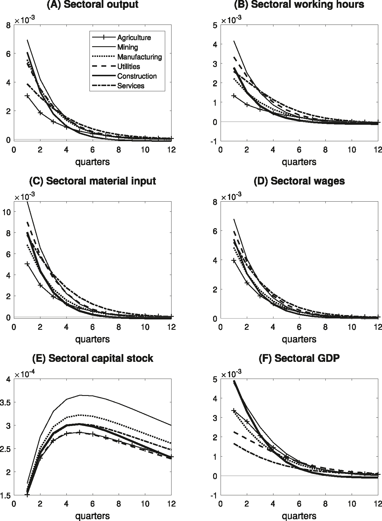
Impulse responses to a monetary policy shock. Notes: The figures illustrate the dynamic responses of sectoral outputs, hours worked, material input, wages, capital stock, and GDP in response to a loosening of monetary policy shock of 50 basis points per annum. The X-axis represents the number of quarters following the monetary policy shock. The Y-axis denotes the magnitude of responses to the monetary policy shock in log points.
Panels (G) and (H) in Figure 2 show sectoral relative prices and consumption responses, respectively. The decline in the relative price of Services arises because its nominal price is the most rigid among the six production sectors. The increase in nominal service prices is smaller than those in other sectors, and thus, its relative price declines. In contrast, the relative prices of other sectors, whose nominal prices are relatively flexible, rise. The differences in sectoral consumption responses are due to changes in relative prices, which arise from the differences in price rigidities. The responses show that household consumption expands least for goods whose relative prices increase the most. The consumption of the agricultural products even contracts for the first two quarters after the shock. In this sense, the change in the consumption basket composition mainly reflects intra-temporal substitution by households.
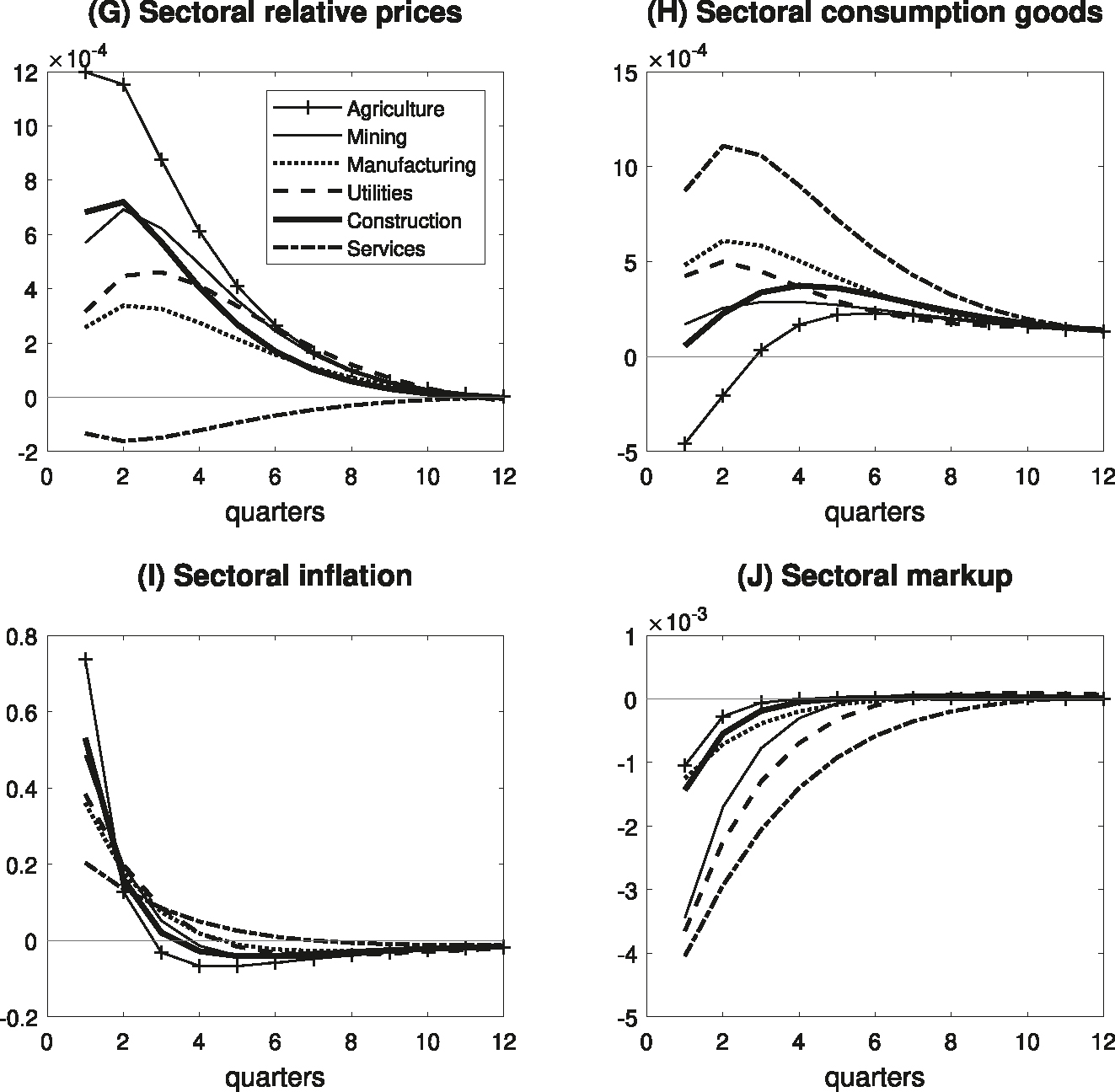
Impulse responses to a monetary policy shock (continued). Notes: The figures illustrate the dynamic responses of sectoral relative prices, consumption goods production, inflation, and markup in response to a loosening of monetary policy shock of 50 basis points per annum. The X-axis represents the number of quarters following the monetary policy shock. The Y-axis denotes the magnitude of responses to the monetary policy shock in log points, except for the inflation whose deviations are expressed in percentage points per annum.
Panel (I) plots the responses of inflation rates to the monetary policy shock. The inflation rates of all sectors increase after the monetary shock, but the increase is more evident in sectors with flexible price settings. In contrast, Services inflation rises less, but it is most persistent. The responses of markups are plotted in Panel (J), which shows that the sectors with relatively rigid prices, such as Services, Utilities, and Mining, record larger declines. This reflects that the markups decrease to a greater extent in sectors with rigid prices as retailers find it difficult to pass through wholesale price increases on to retail prices.
The responses of the interest rates and aggregate inflation rate are plotted in Panel (K) in Figure 3. The response of the nominal interest rate is reduced as a result of the monetary policy easing shock. Since then, the nominal policy rate has gradually returned to the initial level, reflecting the positive inflation gap and GDP gap. As the nominal interest rate falls and the inflation rate rises, the real interest rate decreases, which brings about an expansionary effect on the economy. Panel (L) shows the responses of aggregate output, hours worked, and material input. The capital stock, which is presented in Panel (M), shows slow-moving adjustment, peaking at most five quarters after the shock. Panel (N) plots aggregate GDP and its expenditure components, consumption and investment. The relative deviations of the GDP and its components are consistent with stylized facts regarding business cycles.
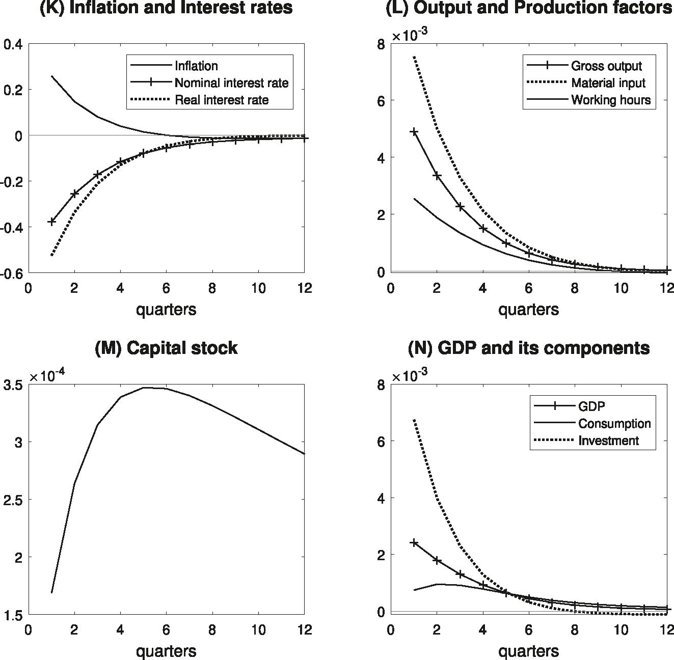
Impulse responses to a monetary policy shock (continued). Notes: The figures illustrate the dynamic responses of aggregate inflation, interest rates, output, capital stock, and aggregate GDP and its components in response to a loosening of monetary policy shock of 50 basis points per annum. The X-axis represents the number of quarters following the monetary policy shock. The Y-axis denotes the magnitude of responses to the monetary policy shock in log points, except for the inflation and interest rates whose deviations are expressed in percentage points per annum.
4.2 The Sources of the Asymmetric Transmission
The expansionary monetary policy shock generates a rise in aggregate demand, which in turn expands aggregate output. This increase is not evenly spread across sectors mainly due to the following reasons. First, the difference in price rigidities across sectors affects the extent to which each industry accommodates the expanded demand by increasing its production. It is expected that the sectors with stickier price-setting would increase their output to a larger extent compared to those with relatively flexible price-setting. Second, sectoral products are demanded, either for building up capital stock or using them as material inputs in their own or other sectors' production as determined by the Input–Output structure of the economy. This implies that production would increase further for the sectors whose outputs are extensively used as material inputs or investment goods in the production processes. These two factors are the sources of the asymmetric transmission of monetary policy as shown in the baseline output response (Panel (A) in Figure 1).
To investigate the operation of the two channels, I simulate the model with one of the two channels deactivated. First, I assume that all industries have the same degree of price stickiness, and therefore, any asymmetric output response stems from the differences in inter-industry linkages and production technologies across sectors. The results are presented in Figure 4. I find that the responses on impact are closely related to the use of produced goods of each industry. To be specific, the larger the portion of produced goods used in production process as material inputs or investment goods, the greater the impact on output due to the expanded demand stemming from the Input–Output linkage effect. The responses on impact are roughly proportional to the share of output used as material and investment goods. For example, relatively large output responses in Mining and Construction reflect that almost all final goods in those sectors are consumed as material inputs and investment goods, respectively.
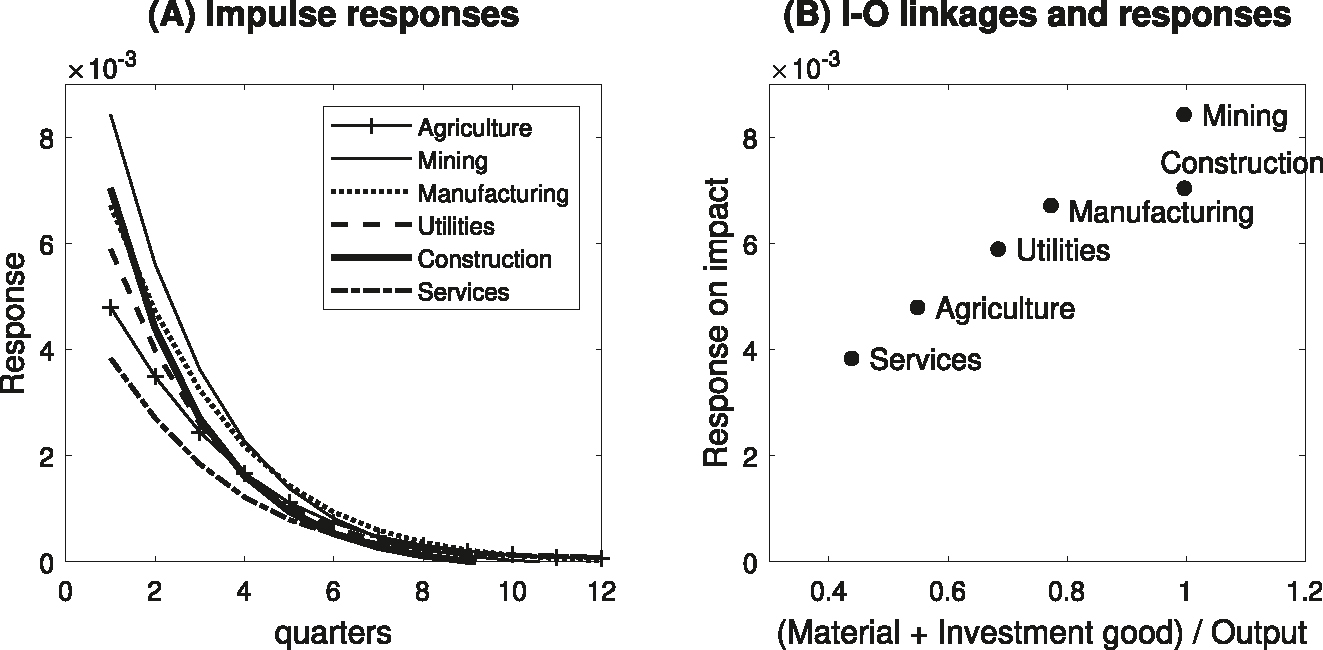
Conditional responses: Homogeneous price stickiness. Notes: The figures are simulation results from a model where all six sectors have the same value for the price stickiness parameter, that is, ϑ h = 0.731 for all h, reflecting an average price duration of 3.71 quarters. Panel (A) presents the dynamic responses of sectoral output in response to a loosening of monetary policy shock of 50 basis points per annum. The X-axis represents the number of quarters following the monetary policy shock. The Y-axis denotes the magnitude of responses to the monetary policy shock in log points. Panel (B) shows the relationship between the ratio of output in each sector used as material input or investment goods and the sectoral output response on impact.
Figure 5 presents the simulation results from the model in which inter-industry linkages and production technologies are restricted to be symmetric across sectors. The matrices determining Input–Output relations are set as identity matrices, which means that each production sector does not rely on goods produced in other sectors in its production process. For the factor intensity coefficients in the production functions, the estimates for the entire economy are used in all sectors. It is also assumed that the portion of each industry’s output in the household’s consumption basket is 1/6. Because of the symmetry in the production technologies and inter-industry linkages, any differences in output responses would reflect those in sectoral price stickiness. I find that the magnitude of the responses on impact is determined by the sectoral price stickiness. For example, Services, which has the stickiest price-setting, shows the largest output response.
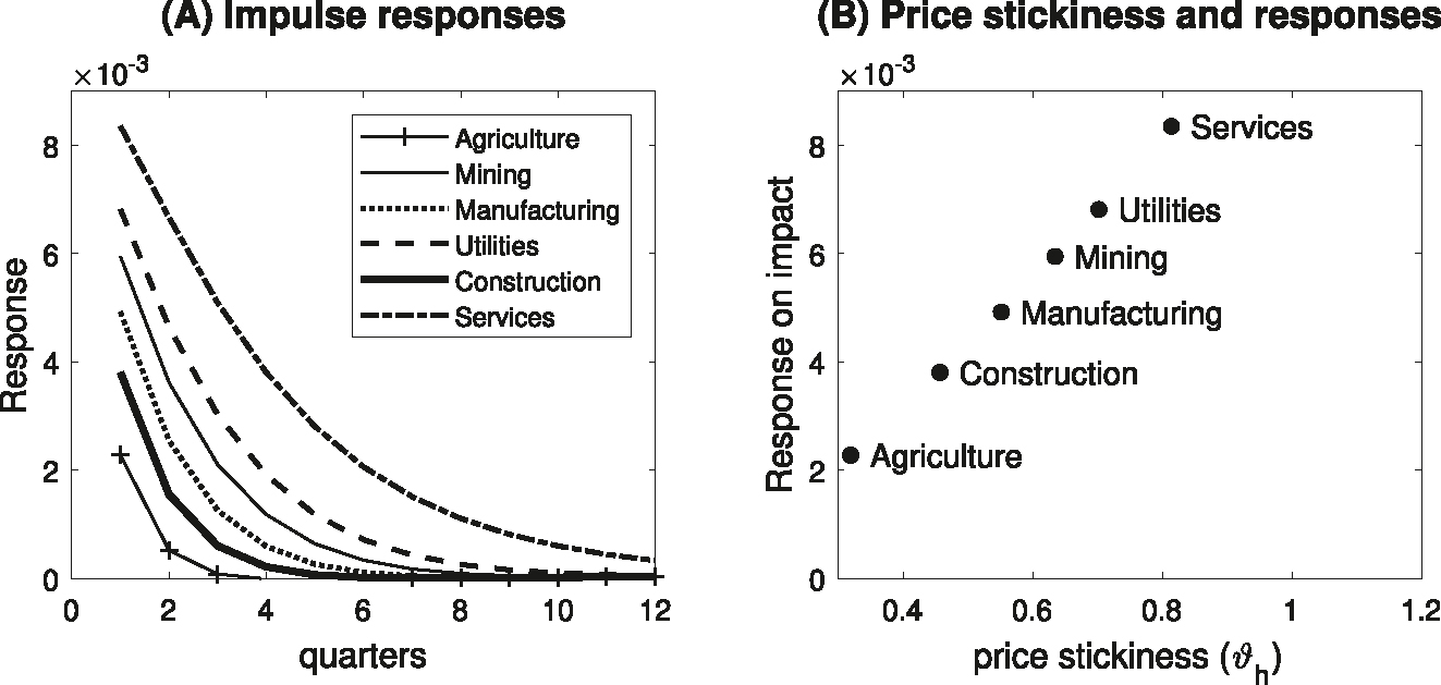
Conditional responses: Homogeneous production sectors and Input-Output linkages off. Notes: The figures are simulation results from a model where all six sectors have the same production technology and Input-Output linkages across sectors are shut off. The matrices determining Input–Output relations are set as identity matrices, implying that each production sector does not rely on goods from other sectors in its production process. Panel (A) presents the dynamic responses of sectoral output in response to a loosening of monetary policy shock of 50 basis points per annum. The X-axis represents the number of quarters following the monetary policy shock. The Y-axis denotes the magnitude of responses to the monetary policy shock in log points. Panel (B) shows the relationship between sectoral price stickiness and the sectoral output response on impact.
I can infer which of these two sources primarily works for each sector. The relatively large output responses in Mining and Construction stem from the fact that their final products are used mainly as material inputs or investment goods, respectively. In the cases of Manufacturing and Utilities, the responses reflect relatively higher proportions of final products being demanded as production factors. Despite the most rigid price-setting behavior, Services shows relatively subdued responses because a substantial portion of its products are used for final consumption. As prices in Agriculture are most flexible and its final products are not substantially used in the production processes compared to other sectors, its output expansion is smallest.
When sectors are ranked by output response magnitudes, the order in our study is Mining-Construction-Manufacturing-Utilities-Services-Agriculture. In contrast, the order in the U.S. case is Services-Construction-Nondurable Manufacturing-Durable Manufacturing-Agriculture-Mining (Bouakez et al. 2009). A notable feature is that while Services exhibit the largest response in the U.S., they belong to the group with relatively smaller responses in our study. In the U.S., the degree of price rigidity in the service sector significantly exceeds that of other sectors, resulting in the largest response despite services being used primarily as consumption goods. In Korea, the difference in price rigidity between services and other sectors is smaller, so the effect of the industrial linkage outweighs the price rigidity effect, resulting in a relatively smaller output response of services.
4.3 Comparison to a Single Sector Model
For comparison purposes, I construct a standard sticky-price DSGE model that features a single producing sector. The production factors in this model include labor and capital stock, but not material input. The factor intensities for labor and capital stock are derived from the estimates for the entire economy (as reported in Table 3) and are adjusted proportionally to sum to one. The adjusted factor coefficients are 0.581 for labor and 0.419 for capital stock. For price stickiness, the value for the entire economy, which is the average price durations of the six production sectors, is used. To be specific, the price stickiness parameter is 0.731, which means that prices remain unchanged for 3.71 quarters on average (See Section 3.3).
Figure 6 compares the responses of aggregate production and inflation from the multisector model and the single-sector model. In the single-sector model, output and GDP are indistinguishable because no material input is used in the production process. In comparison with the baseline multisector version, GDP shows a slightly larger initial response but it is less persistent. In terms of gross output, the response from the single-sector model is roughly half that from multisector model. The inflation response is nearly double that of the multisector model. This implies that ignoring the Input–Output linkages and differences in price stickiness lead to a downward bias in output response and an upward bias in inflation response.
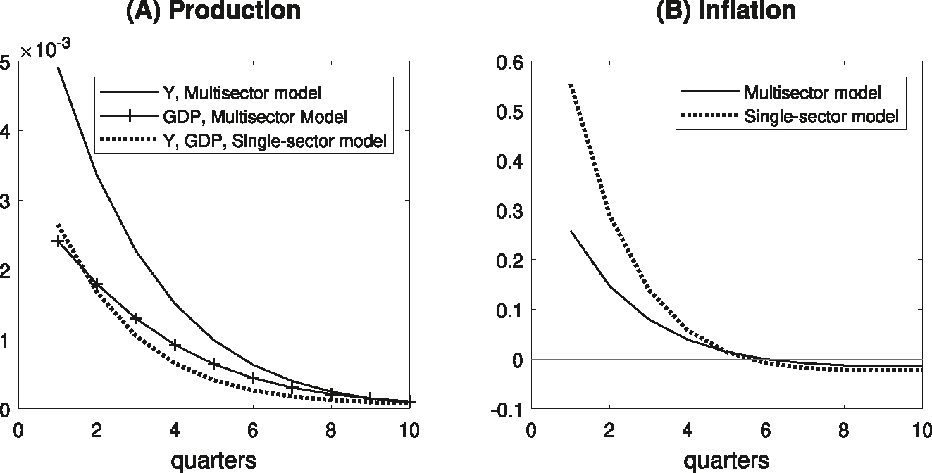
Multisector model versus single-sector model. Notes: The figures illustrate the dynamic responses of aggregate production and inflation in response to a loosening of monetary policy shock of 50 basis points per annum in the multisector model (baseline results) and a counterfactual single-sector model. The X-axis represents the number of quarters following the monetary policy shock. The Y-axis denotes the magnitude of responses to the monetary policy shock in log points for production and percentage points per annum for inflation.
5 Conclusions
The primary objective of monetary authorities is to stabilize aggregate inflation and output rather than to target the dynamics of corresponding sectoral variables. However, it is still crucial for central bankers to understand the transmission of monetary policy across different production sectors in order to obtain precise estimates of how monetary actions affect the entire economy that they are aiming to stabilize. The dynamics of aggregate output and inflation responses to monetary policy could vary as interactions across heterogeneous industry sectors take place. It is also important to predict the consequences of monetary policy on sectoral production and employment, particularly when business cycles in some sectors diverge from those of other sectors or from the broader economy, or when industry-specific economic problems emerge. In this study, I examined the role of sectoral heterogeneities in terms of price rigidity and inter-industry production linkages across the six industry sectors in Korea by using a multisector production NK-DSGE model. The findings in this paper show that substantial sectoral differences exist in terms of price rigidities and inter-industry production linkage effects, and these two aspects were found to be important sources that generate an asymmetric impact of monetary policy decisions. The results imply that policymakers should bear in mind that quantitative estimates of monetary policy impacts could be distorted if they rely on single production sector models that do not consider the sectoral heterogeneities and production linkage effects.
Funding source: National Research Foundation of Korea (NRF)
Award Identifier / Grant number: No. 2023S1A5A807737211
Acknowledgments
I am grateful to the journal editor, Arpad Jeno Abraham, and two anonymous referees for their helpful comments and suggestions.
-
Research funding: This work was supported by the National Research Foundation of Korea (NRF) grant funded by the Korean government (No. 2023S1A5A807737211).
Appendix A: Data Sources
Input–Output structure: Input–Output Tables (IOTs) 2021 edition, OECD; Capital Formation by Activity ISIC rev4, 2019 archive, OECD, Estimation of Production Function Parameters: Gross Value Added and Factor Income by Economic Activities (current prices, annual), National Accounts, The Bank of Korea; Productive Capital Stock by Economic Activities (current prices, year-end), National Balance Sheets, The Bank of Korea, Bayesian Estimation: Monetary policy rate: Call Rate, overnight, intermediated transactions, The Bank of Korea; Consumer Price Index (CPI), Statistics Korea; Sectoral inflation: Producer Price Index (PPI), The Bank of Korea; Wages: Survey on Labor Force at Establishments, Ministry of Employment and Labor; Aggregate Gross Domestic Product (GDP) and Household Consumption: Real GDP (chained 2015 prices), National Accounts, The Bank of Korea; Population: Projected Population by Age, Statistics Korea.
References
Acemoglu, Daron, Ufuk Akcigit, and William Kerr. 2016. “Networks and the Macroeconomy: An Empirical Exploration.” NBER Macroeconomics Annual 30: 273–335. https://doi.org/10.1086/685961.Suche in Google Scholar
Acemoglu, Daron, Vasco M. Carvalho, Asuman Ozdaglar, and Alireza Tahbaz-Salehi. 2012. “The Network Origins of Aggregate Fluctuations.” Econometrica 80 (5): 1977–2016.10.3982/ECTA9623Suche in Google Scholar
Barth, III, J. Marvin, and Valerie A. Ramey. 2001. “The Cost Channel of Monetary Transmission.” NBER Macroeconomics Annual 16: 199–240. https://doi.org/10.1086/654443.Suche in Google Scholar
Bernanke, Ben S., Mark Gertler, and Simon Gilchrist. 1999. “The Financial Accelerator in a Quantitative Business Cycle Framework.” In Handbook of Macroeconomics, Vol. 1: 1341–93. Amsterdam: Elsevier Science Publishers B.V.10.3386/w6455Suche in Google Scholar
Bils, Mark, and Peter J. Klenow. 2004. “Some Evidence on the Importance of Sticky Prices.” Journal of Political Economy 112 (5): 947–85, https://doi.org/10.1086/422559.Suche in Google Scholar
Bouakez, Hafedh, Emanuela Cardia, and Francisco J. Ruge-Murcia. 2009. “The Transmission of Monetary Policy in a Multisector Economy.” International Economic Review 50 (4): 1243–66, https://doi.org/10.1111/j.1468-2354.2009.00567.x.Suche in Google Scholar
Bouakez, Hafedh, Emanuela Cardia, and Francisco J. Ruge-Murcia. 2011. “Durable Goods, Inter-sectoral Linkages and Monetary Policy.” Journal of Economic Dynamics and Control 35 (5): 730–45, https://doi.org/10.1016/j.jedc.2010.12.013.Suche in Google Scholar
Bouakez, Hafedh, Emanuela Cardia, and Francisco Ruge-Murcia. 2014. “Sectoral Price Rigidity and Aggregate Dynamics.” European Economic Review 65: 1–22. https://doi.org/10.1016/j.euroecorev.2013.09.009.Suche in Google Scholar
Calvo, Guillermo A. 1983. “Staggered Prices in a Utility-Maximizing Framework.” Journal of Monetary Economics 12 (3): 383–98, https://doi.org/10.1016/0304-3932(83)90060-0.Suche in Google Scholar
Carvalho, Carlos. 2006. “Heterogeneity in Price Stickiness and the Real Effects of Monetary Shocks.” Frontiers of Macroeconomics 2 (1). https://doi.org/10.2202/1534-6021.1320.Suche in Google Scholar
Christiano, Lawrence J., Martin Eichenbaum, and Charles L. Evans. 2005. “Nominal Rigidities and the Dynamic Effects of a Shock to Monetary Policy.” Journal of Political Economy 113 (1): 1–45, https://doi.org/10.1086/426038.Suche in Google Scholar
Dedola, Luca, and Francesco Lippi. 2005. “The Monetary Transmission Mechanism: Evidence from the Industries of Five OECD Countries.” European Economic Review 49 (6): 1543–69, https://doi.org/10.1016/j.euroecorev.2003.11.006.Suche in Google Scholar
Ferrante, Francesco, Sebastian Graves, and Matteo Iacoviello. 2023. “The Inflationary Effects of Sectoral Reallocation.” Journal of Monetary Economics 140: s64–s81.10.1016/j.jmoneco.2023.03.003Suche in Google Scholar
Ghassibe, Mishel. 2021. “Monetary Policy and Production Networks: An Empirical Investigation.” Journal of Monetary Economics 119: 21–339.10.1016/j.jmoneco.2021.02.002Suche in Google Scholar
Horvath, Michael. 1998. “Cyclicality and Sectoral Linkages: Aggregate Fluctuations from Independent Sectoral Shocks.” Review of Economic Dynamics 1 (4): 781–808, https://doi.org/10.1006/redy.1998.0028.Suche in Google Scholar
Horvath, Michael. 2000. “Sectoral Shocks and Aggregate Fluctuations.” Journal of Monetary Economics 45 (1): 69–106, https://doi.org/10.1016/s0304-3932(99)00044-6.Suche in Google Scholar
La’O, Jennifer and Alireza, Tahbaz-Salehi. 2022. “Optimal Monetary Policy in Production Networks.” Econometrica 90: 1295–1336.10.3982/ECTA18627Suche in Google Scholar
Lee, Seungyoon, and Jongwook Park. 2022. “Identifying Monetary Policy Shocks Using Economic Forecasts in Korea.” Economic Modelling 111: 105803. https://doi.org/10.1016/j.econmod.2022.105803.Suche in Google Scholar
Lee, Seungyoon, and Jongwook Park. 2025. “Business Cycles, Monetary Policy Stance, and Monetary Policy Transmission in Korea.” The B.E. Journal of Macroeconomics. https://doi.org/10.1515/bejm-2024-0127.Suche in Google Scholar
Nakamura, Emi, and Jón Steinsson. 2008. “Five Facts About Prices: A Reevaluation of Menu Cost Models.” Quarterly Journal of Economics 123 (4): 1415–64, https://doi.org/10.1162/qjec.2008.123.4.1415.Suche in Google Scholar
Nakamura, Emi, and Jon Steinsson. 2010. “Monetary Non-neutrality in a Multisector Menu Cost Model.” Quarterly Journal of Economics 125 (3): 961–1013, https://doi.org/10.1162/qjec.2010.125.3.961.Suche in Google Scholar
Pasten, Ernesto, Raphael Schoenle, and Michael Weber. 2020. “The Propagation of Monetary Policy Shocks in a Heterogeneous Production Economy.” Journal of Monetary Economics 116: 1–22. https://doi.org/10.1016/j.jmoneco.2019.10.001.Suche in Google Scholar
Peersman, Gert, and Frank Smets. 2005. “The Industry Effects of Monetary Policy in the Euro Area.” The Economic Journal 115 (503): 319–42, https://doi.org/10.1111/j.1468-0297.2005.00991.x.Suche in Google Scholar
Petrella, Ivan, Raffaele Rossi, and Emiliano Santoro. 2019. “Monetary Policy with Sectoral Trade-Offs.” The Scandinavian Journal of Economics 121 (1): 55–88, https://doi.org/10.1111/sjoe.12266.Suche in Google Scholar
Smets, Frank, and Rafael Wouters. 2007. “Shocks and Frictions in US Business Cycles: A Bayesian DSGE Approach.” The American Economic Review 97 (3): 586–606, https://doi.org/10.1257/aer.97.3.586.Suche in Google Scholar
The Bank of Korea. 2017. Monetary Policy in Korea. https://www.bok.or.kr/eng/bbs/E0000742/view.do?nttId=234109&searchCnd=1&searchKwd=&depth2=400066&depth=400066&pageUnit=10&pageIndex=1&programType=newsDataEng&menuNo=400224&oldMenuNo=400066.Suche in Google Scholar
© 2025 the author(s), published by De Gruyter, Berlin/Boston
This work is licensed under the Creative Commons Attribution 4.0 International License.
Artikel in diesem Heft
- Frontmatter
- Advances
- Real Wage Cyclicality and Monetary Policy
- Green Transition, Skills Heterogeneity, and Inequality
- Workforce Aging, Growth and Productivity
- Monetary Policy Shocks: Data or Methods?
- Contributions
- Monetary Policy and Labor Market Friction in a HANK Model
- Capital Market Liberalization and Bank Credit Decisions: A Quasi-Natural Experiment Based on the “Mainland-Hong Kong Stock Connect”
- Automation, Skill Premium, and Labor Share
- Business Cycles, Monetary Policy Stance, and Monetary Policy Transmission in Korea
- Forecasting Revisions to U.S. Jobs Report Data
- Loan Loss Provision, Unsecured-Collateralized Loan Choice and Macro-Stability in China
- Price Stickiness, Input–Output Linkages, and Monetary Policy Transmission in Korea
- Oil Price-Driven Inflation and the Channels of Pass-Through
- Firm Dynamics, Informality, and Monetary Policy