Business Cycles, Monetary Policy Stance, and Monetary Policy Transmission in Korea
-
Seungyoon Lee
 und
Jongwook Park
und
Jongwook Park


Abstract
This paper investigates the asymmetric transmission of monetary policy across business cycles in Korea during the period following the global financial crisis. Utilizing a smooth transition-local projection regression method, we explore the asymmetric responses of output and prices to monetary policy shocks during economic booms and recessions. Monetary policy innovations are identified by orthogonalizing changes in the policy rate with respect to economic forecast information that policymakers consider in their decision-making processes. Our findings reveal that the impact of monetary policy on output and prices is substantial during recessions, whereas it is minimal and statistically insignificant during booms. By examining asymmetries arising from both business conditions and monetary policy stance, we show that the pronounced transmission effects during recessions are primarily driven by tightening monetary policy, while expansionary measures during recessions have limited effectiveness. These results suggest the need to reevaluate previous empirical findings which do not simultaneously consider the possibility of asymmetric transmission stemming from both business cycles and monetary policy stance.
1 Introduction
Since the global financial crisis, the effectiveness of monetary policy has become a central issue for macroeconomists and policy makers. Despite unprecedented large-scale monetary easing, economic recovery has been delayed, and inflation rates have remained below target for an extended period, raising concerns about the efficacy of monetary policy as a stabilization tool. Addressing this issue requires considering the possibility that monetary policy transmission depends on economic conditions, as many studies have reported that business cycles matter in the transmission. This study goes beyond merely considering business cycles to analyze whether the effects of monetary policy varies with its stance – whether monetary policy is tightening or loosening – across different phases of business cycles. The significance of this research lies in incorporating both business cycles and monetary policy stance into the empirical analysis of policy transmission effects, questioning the conventional expectation that expansionary monetary policy is implemented during recessions and contractionary policy during expansions.
We first examine whether the effects of monetary policy vary across business cycles in Korea after the global financial crisis. Korea is chosen for analysis due to the applicability of our method for identifying monetary policy shocks, considering data availability and the overall framework of monetary policy implementation. Previous reports indicate that monetary policy transmission in Korea has been effective in the post-crisis period based on a conventional linear regression model, making it suitable for investigating asymmetric transmission across business cycles.[1] To examine the responses of output and prices to monetary policy shocks across business cycles, we use a smooth transition-local projection regression, incorporating a state variable representing each phase of business cycles into an autoregressive distributed lag model. This approach enables us to measure the responses of output and prices to monetary policy innovations in both booms and recessions within a unified framework. The standardized series of the cyclical component of coincident composite index, representing overall business conditions, is used as the state variable. Monetary policy innovations are identified by orthogonalizing changes in the policy rate with respect to economic forecasts considered by policymakers (Romer and Romer 2004; Cloyne and Hürtgen 2016; Lee and Park 2022).
In our experiments, the effects of monetary policy on output and prices were substantial and significant in recessions but small and insignificant in booms. During booms, the responses of industrial production and the consumer price index were unclear or contrary to expectations. In contrast, the responses in recessions were quantitatively substantial and statistically significant. These results suggest that the evident transmission of monetary policy in Korea previously documented in a linear model has been primarily driven by that implemented in recessions, with monetary policy remaining ineffective in booms. These findings remain consistent when adopting alternative specifications for identifying monetary policy shocks and business cycle indicators as well as alternative sample periods. Our results are not explained by the theory of a convex aggregate supply curve that is a conventional explanation predicting greater output responses in recessions and greater price responses in booms.
We then investigate whether tightening shocks and loosening shocks have different effects on the economy across business cycle phases. Examining whether responses depend on the signs of monetary policy shocks, we find that in recessions, tightening monetary policy has a substantial impact, while loosening policy has little effect. In booms, expansionary policy has a significant impact, but the effectiveness of tightening policy is unclear or weak. These results imply that the notable monetary policy transmission observed in recessions is primarily due to contractionary policies rather than expansionary policies typically expected in downturns.
Finally, to understand the causes of asymmetric transmission, we examine how financial characteristics in manufacturing subsectors are related to production adjustments in response to monetary policy shocks. Specifically, we construct firm-level indicators representing financial conditions or balance sheet strength (e.g., leverage, operating profits over interest payments, short-term debt over total debt) to examine whether responses depend on these financial variables. We find that more leveraged industries experienced smaller contractions, suggesting that higher leverage ratios indicate greater borrowing capacity, facilitating external funding access. This relationship is apparent in booms, but not in recessions, indicating that high leverage ratios amplify asymmetric effects across business cycle phases.
Several studies on the state-dependent transmission across business cycles have documented greater transmission in recessions in the U.S. (Weise 1999; Garcia and Schaller 2002; Lo and Piger 2005) and the Euro area (Peersman and Smets 2001, 2005), while others find stronger effects in booms in the U.S. (Tenreyro and Thwaites 2016) and in advanced or emerging economies (Hang and Xue 2020; Alpanda et al. 2021). Previous studies also explore sign-dependent transmission, with findings documenting that contractionary policies impact output more than expansionary policies (De Long et al. 1988; Cover 1992; Morgan 1993; Karras 1996a,b; Karras and Stokes 1999; Barnichon, Matthes, and Timothy 2017; Angrist, Jordà, and Kuersteiner 2018; Barnichon and Matthes 2018; Debortoli et al. 2020; Jordà, Singh, and Taylor 2020). A few studies have not found asymmetric effects based on the sign of monetary policy innovations (Weise 1999; Ravn and Sola 2004; Lo and Piger 2005).
Our research is distinct in examining asymmetric transmission in terms of both business cycle phases and monetary policy stance. Existing studies focus on either business cycle phases or the sign of policy innovations, which may lead to incorrect judgments regarding the effectiveness of monetary policy. It is typically assumed a prior relationship between the direction of monetary policy and business conditions: expansionary policy during recessions and contractionary policy during booms. This conventional belief may lead to the conclusion that monetary policy is an effective stabilizing tool, based on the strong transmission observed during recessions. However, there is no clear correlation between the signs of identified monetary policy innovations and business cycle phases. In fact, positive innovations (contractionary shocks) are often observed in recessions and negative innovations (expansionary shocks) in booms. Monetary authorities might tolerate greater output and inflation volatility to achieve broader targets like financial stability and external balance. Central banks may implement tightening amid cost-push shocks and stagnation. Our findings that influential effects in recessions are mainly due to tightening policy necessitate considering both policy stance and business cycle phases simultaneously, justifying a re-examination of previous evidence on transmission.
The remainder of the paper is structured as follows: Section 2 describes the methodology for identifying monetary policy shocks and business cycle phase indicators. Section 3 presents evidence on state-dependent transmission across business cycles. Section 4 examines contractionary and expansionary transmission in booms and recessions. Section 5 investigates financial characteristics in manufacturing subsectors related to production adjustments. Section 6 concludes.
2 Measurement of Monetary Policy Shocks and Business Cycles
We describe the methodology for identifying monetary policy innovations in Section 2.1. We construct a smooth transition indicator for business cycles in Section 2.2.
2.1 Monetary Policy Shock Identification
We identify monetary policy shocks following Romer and Romer’s narrative approach, in which changes in the policy rate that are not systematically related to economic forecast information are regarded as monetary policy shocks (Romer and Romer 2004; Cloyne and Hürtgen 2016; Lee and Park 2022). To be specific, monetary policy shocks are identified by orthogonalizing changes in the policy rate with respect to economic forecast information on the latest developments of output and prices that policymakers have when they make monetary policy decisions. The regression specification for identifying monetary policy shocks is as follows:
where m represents the monetary policy decision meeting, and j refers to the horizon of the forecast: −1 is the previous quarter; 0 is the current quarter; and 1 and 2 are one and two quarters ahead, respectively. The dependent variable,
This identification methodology is appropriate for the Korean case as the monetary authority in Korea, the Bank of Korea, has implemented monetary policy under the so-called inflation targeting framework in our sample period, referring to forecast information in determining its policy rate. As is well known, economic growth and inflation forecasts constitute key information variables for preemptive monetary policy implementation. The Bank of Korea has publicly announced its forecast information immediately after its policy decision meetings, thus minimizing the informational gap between policymakers and private agents. As private agents can instantly refer to economic forecasts when interpreting monetary policy decisions, any change in the policy rate that cannot be systematically explained by forecast information constitutes a surprise monetary policy innovation.
The regression is implemented for a sample of 120 monetary policy decision-making meetings between January 2009 and December 2019. We gather forecasts and the latest real-time data by reading the historical archives of Main Economic Indicators and Economic Outlook. The former is the Bank of Korea’s internal report prepared for policy decision-making meetings, which includes the latest information on comprehensive macroeconomic variables such as GDP and its components, production, and prices. The latter is the Bank of Korea’s official economic forecast, which the bank’s internal staff produces four times a year. Table 1 shows the regression results.[2] The coefficient on the policy rate from the previous meeting (−0.068) is estimated to be negative, suggesting a mean-reverting pattern in policy decisions. The estimated coefficients on output growth (0.032) and inflation (0.080) indicate that it tends to raise the policy rate in response to expected increases in either variable.
Estimation results of monetary policy shock identification regression.
| j | Coefficient | s.e. | t-statistics | |
|---|---|---|---|---|
| Intercept | −0.062 | 0.047 | −1.315 | |
| Target from the last meeting
|
−0.068** | 0.030 | −2.268 | |
| Forecast output growth
|
−1 | −0.003 | 0.015 | −0.209 |
| 0 | −0.009 | 0.022 | −0.409 | |
| 1 | 0.035* | 0.019 | 1.798 | |
| 2 | −0.002 | 0.023 | −0.074 | |
| Total Effect | 0.021 | 0.019 | 1.113 | |
| Output revision
|
−1 | 0.047** | 0.023 | 2.085 |
| 0 | −0.004 | 0.035 | −0.126 | |
| 1 | 0.026 | 0.073 | 0.355 | |
| 2 | −0.058 | 0.060 | −0.971 | |
| Total Effect | 0.011 | 0.030 | 0.371 | |
| Output | Total Effect | 0.032 | 0.029 | 1.118 |
| Forecast inflation
|
−1 | −0.009 | 0.034 | −0.263 |
| 0 | 0.033 | 0.055 | 0.595 | |
| 1 | −0.015 | 0.037 | −0.408 | |
| 2 | 0.047 | 0.043 | 1.075 | |
| Total Effect | 0.055* | 0.029 | 1.910 | |
| Inflation revision
|
−1 | 0.085 | 0.049 | 1.725 |
| 0 | −0.091 | 0.104 | −0.875 | |
| 1 | 0.122 | 0.131 | 0.930 | |
| 2 | −0.091 | 0.110 | −0.827 | |
| Total Effect | 0.025 | 0.065 | 0.386 | |
| Inflation | Total Effect | 0.080 | 0.062 | 1.287 |
-
The table presents estimation results of the monetary policy shock identification regression. The complete regression specification for Equation (1) is as follows:
Panel (A) in Figure 1 plots the identified monetary policy shocks and changes in the policy rate. Overall, both series move in the same direction, and their correlation coefficient is quite high (0.854). However, the difference between them is not negligible in some cases. For example, the identified policy shock was quite small (0.035) in July 2010 when the policy rate was increased by 25 basis points. This implies that almost all of the interest rate hike was explained by economic forecast information, indicating the increase was not surprising to the public. In other words, this means that the adjustment in the policy rate at that time could be inferred from the historical relationship between changes in the policy rate and economic forecasts. On the other hand, when the identified monetary policy shock is close in magnitude to the corresponding change in the policy rate, for example, as in March 2015, it indicates that changes in the policy rate significantly deviated from their historical relationship with economic forecasts.
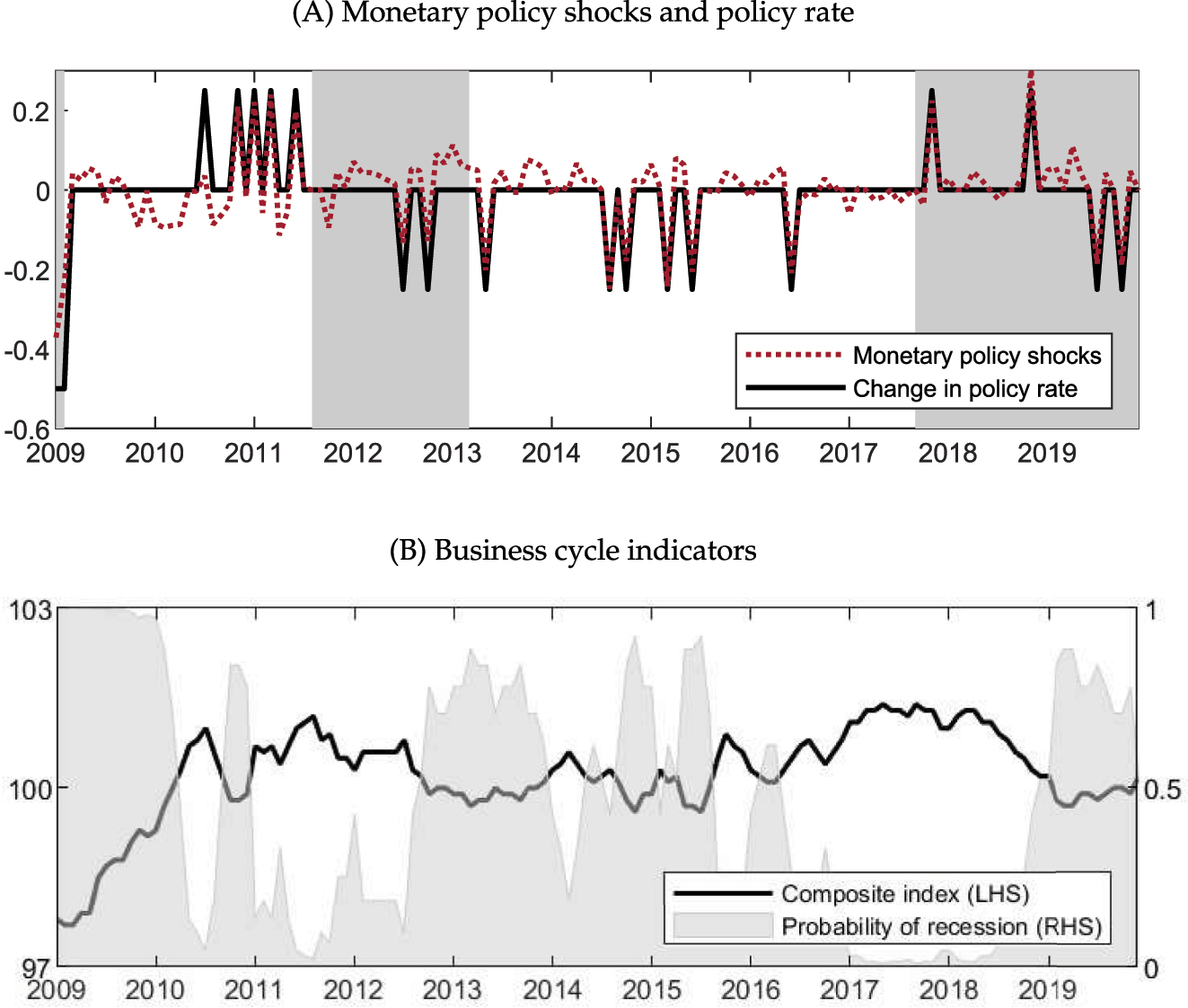
Monetary policy shocks and business cycle indicators. Notes: In Panel (A), the dotted line presents the identified monetary policy shocks. The solid line describes monthly changes of policy rate in Korea (Base Rate). The shaded areas represent official economic contraction in the 9th (Peak: January 2008, Trough: February 2009), 10th (Peak: August 2011, Trough: March 2013), and 11th (Peak: September 2017, Trough: May 2020) business cycle phases arranged by Statistics Korea. In Panel (B), the solid line presents the composite index from National Statistics Office. The shaded areas indicate the probability that the economy is in recessions, computed as 1 − F(z t ).
2.2 An Indicator of Business Cycle Phases
We construct a smooth transition indicator representing the phases of business cycles. Specifically, we transform an indicator of business conditions in the economy, z t , into a logistic function value, F(z t ), as shown below (Granger and Terasvirta 1993; Tenreyro and Thwaites 2016):
where F(z t ) ∈ (0, 1) denotes the probability that the economy is in a boom in time t, while 1 − F(z t ) refers to the probability that the economy is in a recession. c is a parameter that controls the proportion of the sample during which the economy spends in each state and σ z is the standard deviation of the state variable z t . The parameter θ determines how quickly the economy switches from a boom to a recession when z t changes and is set to 3 as in Tenreyro and Thwaites (2016). We use the cyclical component of coincident composite index as z t . The parameter c is set to 100.2, the average value of the cyclical component of composite index for the period of January 2009 to December 2019. The parameter σ z , representing a standard deviation of the cyclical component, is 0.76. Panel (B) in Figure 1 plots the cyclical component of coincident composite index and its transformed value F(z t ). The median and average of F(z t ) during the sample period are 0.57 and 0.53, respectively.
Figure 2 presents the distributions of the identified monetary policy shock series across business cycles. Notably, we do not find any clear-cut correlation between the business cycles and the directions of monetary policy shocks. If the business cycles and the directions of monetary policy shocks were correlated (i.e., loosening monetary policies are dominant in recessions, while tightening policies are dominant in booms), the asymmetric responses across the business cycles might reflect asymmetric transmission of tightening and loosening monetary policies rather than differences in monetary policy effects in economic booms and recessions. The distributional evidence relieves our concerns on this point.
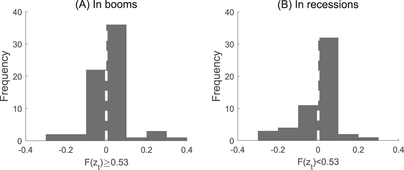
Distribution of monetary policy shocks. Notes: Panel (A) plots the distribution of monetary policy innovations in booms, defined as periods when the smooth logistic function value is greater than 0.53. Panel (B) plots the distribution of monetary policy innovations in recessions, defined as periods when the smooth logistic function value is smaller than 0.53.
3 Monetary Policy Transmission over Business Cycles
We introduce the estimation method in Section 3.1 and interpret the estimation results in Section 3.2. In Section 3.3, we implement a set of robustness tests.
3.1 Estimation Method
We measure the impact of monetary policy across business cycles by estimating the dynamic responses of output and prices to the identified monetary policy shocks. Specifically, we set up a smooth transition-local projection model that allows monetary policy to transmit differently across the business cycle phases (Tenreyro and Thwaites 2016) as follows:
for h = 0, 1, …, H, where y
t
denotes the log-difference of a monthly economic variable,
Note that the state-dependent local projection impulse response estimator may be biased when using an endogenous variable as the state variable, with the degree of bias increasing with the size of the shock (Gonçalves et al. 2024). In this regard, caution should be exercised when interpreting the results of the state-dependent local projection in terms of the absolute magnitude of the impact. In our study, however, the concern has been relieved for the following reasons. First, the purpose of this study is not to quantitatively measure the impacts of monetary policy across business cycles, but rather to compare the differences in them. Second, the state variable in this paper is the cyclical component of coincident composite index, which is not used as an endogenous variable. Third, given that the differences in asymmetric monetary policy transmission across phases are quantitatively significant, we think that this does not compromise the interpretation of our results.
3.2 Baseline Results
Figure 3 presents the estimated dynamic responses of industrial production (IP) and consumer price index (CPI) after a one-unit or 100 basis points of monetary policy shock. The first column shows estimation results from a linear regression model of Equation (2) in which we impose the restriction that monetary policy effects are symmetric across business cycle phases.[3] This is a standard regression model used to measure monetary policy transmission. The second and third columns present the estimation results for booms and recessions, respectively, from Equation (2). The fourth column illustrates the difference in responses between the two business cycle phases.
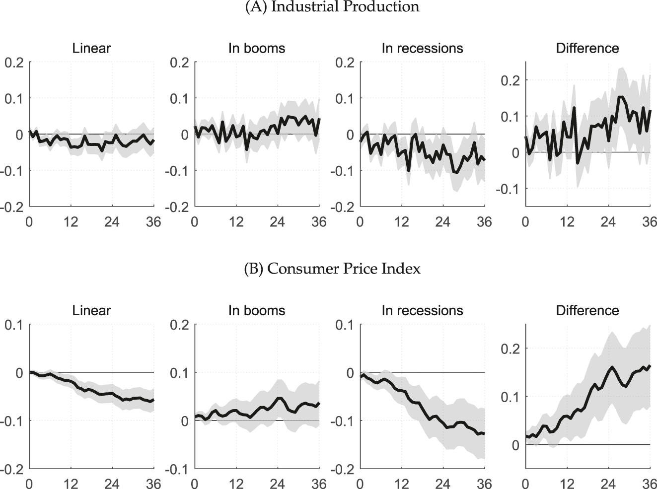
Responses to monetary policy shocks. Notes: The figure plots responses of the industrial production index and consumer price index to monetary policy shocks. The responses are generated by estimating Equation (2) using the local projection procedure. Solid lines represent the estimated responses to one unit of monetary policy shocks. X-axis denotes time horizons (months) and Y-axis denotes the magnitude of responses measured in log points. The responses at horizon h are cumulative responses which add up the responses from period 0 to h. Shaded bands represent one-standard confidence intervals generated from 1,000 times bootstrap replications.
Examining the responses of IP from the linear regression model, it reveals a 4.6 percent decline 21 months after a monetary policy shock. Puzzling increases in initial periods do not appear, and the response is overall significant for the first two years after the shock.[4] When the transmission is allowed to be asymmetric across business cycles, the decline in recessions is larger and statistically significant compared to that in booms. The maximum decline in recessions is 10.6 percent, which is observed 28 months after the shock, and overall, the responses are statistically significant. In contrast, a contraction was not obvious in booms. Except for a borderline significant response at 15 months after a shock, the responses are generally unclear in direction and statistically insignificant. The difference between the responses across business cycle phases is significant.
CPI declines by 6.1 percent after 35 months after a shock in the linear regression model. Puzzling increases in initial periods after a monetary policy shock do not appear, and the CPI continues declining gradually. The responses are substantial and highly significant. Looking at asymmetric transmission across business cycles, the maximum response in recessions is 12.8 percent, occurring 34 months after the shock, which is quantitatively large and statistically significant. In contrast, puzzling increases in the responses in booms exist, though they are not significant. The difference between the responses in booms and those in recessions is quite large and significant.[5]
A convex aggregate supply curve is a conventional explanation for different monetary policy effects in booms and in recessions.[6] With a convex short-run aggregate supply curve, output responses are expected to be larger in recession, while price responses would be smaller in recessions for the same magnitude of change in aggregate demand. In our results, both output and prices respond more significantly in recessions (see Figure 3), which implies that the asymmetric monetary policy transmission we observe cannot be explained by the convex aggregate supply curve theory.
3.3 Robustness Test
We implement a set of alternative regression specifications to check the robustness of our main results.[7] First, we additionally control for forecasts of the unemployment rate and current account in the process of monetary policy shock identification. These variables may include important information on the dynamics of labor market and external trade, which policymakers likely consider when determining the policy rate. Second, we include economic forecasts with a longer forecast horizon, up to three quarters ahead, in the monetary policy shock identification regression. Policymakers might refer to economic forecasts from as longer horizons as possible because monetary policy transmits into the economy in long and variable processes. We do not utilize economic forecasts beyond three quarters due to data availability constraint. Third, we adjust the probability of an economic boom considering uncertainty in business cycle divisions. To be specific, we apply alternative probabilities of a boom by adjusting the parameter, c, representing the average value of the cyclical component of coincident composite index. The average probability was 0.53 in the baseline experiment, and we now examine two alternative business cycle indicators, with the average values set as 0.43 and 0.63, respectively. Fourth, we remove lagged monetary policy shock variables in estimating responses of output and prices. In the baseline regression, lags of monetary policy shocks up to 6 months were included as the endogeneity might not be completely removed in our identification strategy. By removing the lagged variables, we expect to improve the degrees of freedom and the precision of the estimation. Fifth, we drop the sample in the year 2009 as any remaining effect of the crisis turmoil might affect the transmission of monetary policy in normal periods. One rationale for this exercise is that the revision of economic forecasts in 2009 is more volatile compared to those in the sample since 2010. Finally, we control for the impacts of exchange rates in measuring responses of output and prices to monetary policy shocks. Due to the high level of trade openness and a small open economy nature of Korea, changes in the currency value can significantly impact domestic production and price.
The results of these robustness tests are presented in the online Appendix. Our baseline results, showing substantial and significant effects of monetary policy in recessions but not in booms, remain intact.
4 Contractionary versus Expansionary Monetary Policy Transmission
We introduce a regression model that considers not only the business cycle phases but also monetary policy stance, that is, whether monetary policy shocks are contractionary or expansionary, in Section 4.1. We interpret the estimation results in Section 4.2. In Section 4.3, we discuss the policy implications of the results.
4.1 Estimation Method
As discussed earlier, existing studies on asymmetric monetary policy transmission often focus on either the phases of the business cycle or the direction (sign) of monetary policy innovations. However, analyzing only one of these dimensions may lead to incorrect conclusions about monetary policy transmission. For example, examining monetary policy transmission across business cycles without explicitly considering asymmetry due to sign-dependency (as we discussed in Section 3) may lead us to misinterpret the effects of monetary policy during booms and recessions as purely the effects of contractionary and expansionary policies, respectively. This misunderstanding arises because monetary policy is believed to be typically contractionary during booms and expansionary during recessions. However, as shown in Figure 2, there is no clear correlation between business cycle phases and the direction of monetary policy, meaning that it is not always the case. Similarly, focusing solely on the sign-dependence of monetary policy transmission can be misleading if we ignore asymmetric transmission across business cycles. For instance, if we observe a significant impact of tightening monetary policy, we might conclude that it is effective in cooling an overheated economy. This conclusion would be incorrect if, in reality, tightening is effective only during recessions and not during booms. Therefore, it is crucial to consider asymmetric monetary policy transmission from both business conditions and policy direction perspectives, often overlooked in previous studies.
Considering this point, we examine the transmission of contractionary and expansionary monetary policies in economic booms and recessions. To do this, we extend Equation (2) as follows:
We generate two additional monetary policy shock series based on the signs of the monetary policy innovations in each time period: a contractionary monetary policy shock
4.2 Estimation Results
Figure 4 plots the estimation results. The responses of industry production (IP) are shown in Panel (A). In booms, IP does not show clear responses to a contractionary monetary policy shock, but it records significant increases in the first 12 months after an expansionary shock. In recessions, the effect of an expansionary shock on IP is not obvious, while that of a contractionary shock is consistent with our prior expectations.
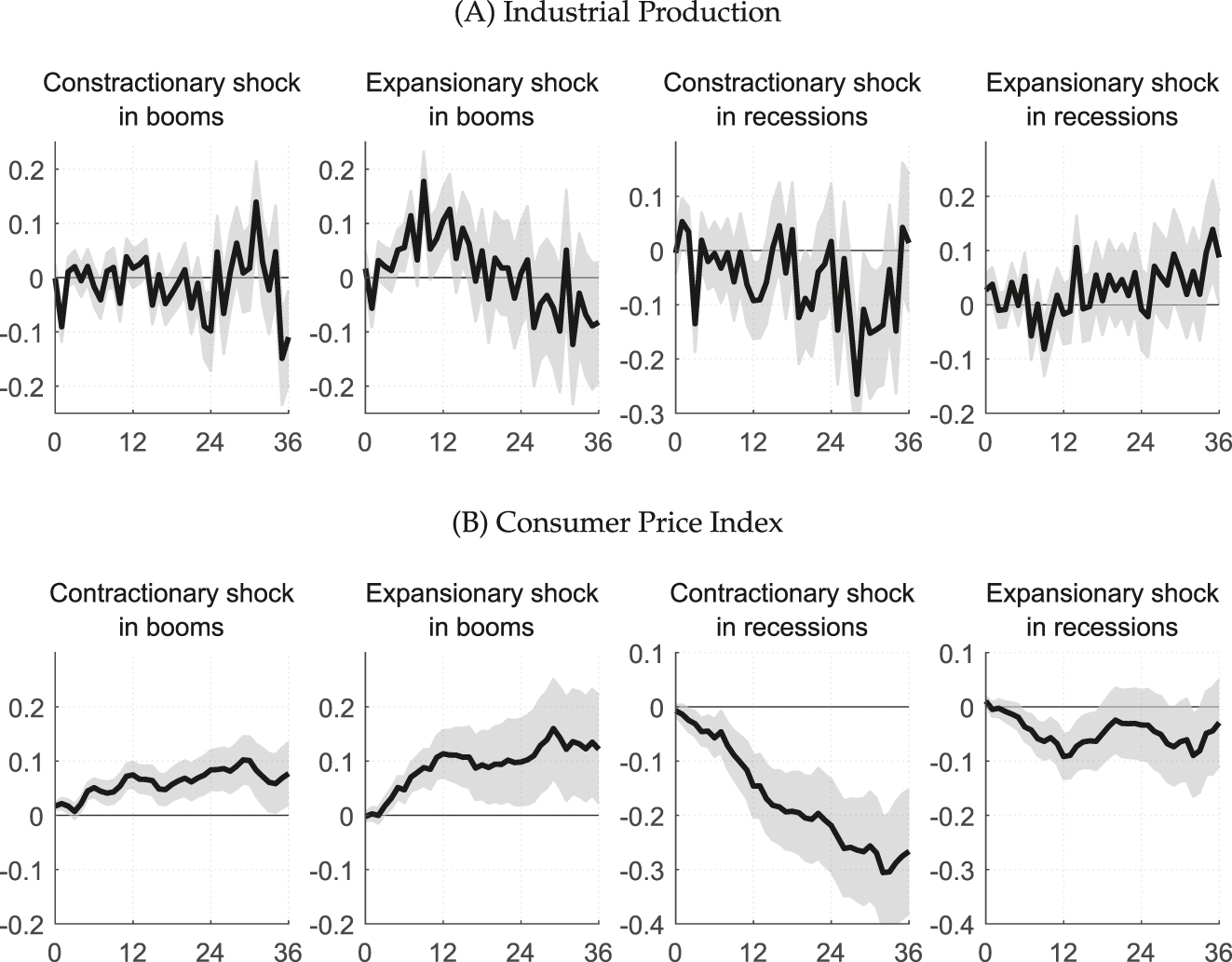
Responses to contractionary and expansionary monetary policy shocks. Notes: The figure plots responses of the industrial production index and consumer price index to monetary policy shocks. The responses are generated by estimating Equation (3) using the local projection procedure. Solid lines represent the estimated responses to one unit of monetary policy shocks. X-axis denotes time horizons (months) and Y-axis denotes the magnitude of responses measured in log points. The responses at horizon h are cumulative responses which add up the responses from period 0 to h. Shaded bands represent one-standard confidence intervals generated from 1,000 times bootstrap replications.
Panel (B) presents the responses of the consumer price index (CPI). The CPI shows responses that are statistically significant and consistent with prior expectations for an expansionary monetary policy shock in booms and a contractionary shock in recession. In contrast, the responses to a contractionary shock in booms and to an expansionary shock in recessions were opposite to our expectations, and these puzzling responses were statistically significant.
In sum, the results imply that the large and significant monetary policy transmission in recessions we observed in Section 3.2 is driven mainly by contractionary monetary policy shocks.[8]
4.3 Policy Implications
Our results prompt a re-evaluation of the conventional view on the effectiveness of monetary policy as a stabilization tool. Without considering the potentially different impacts of monetary easing and tightening, one might conclude that monetary policy effectively stabilizes the economy during recessions, based on the relatively larger responses to monetary policy shocks in recessions compared to booms. However, this conclusion could be misleading, as our results indicate that expansionary monetary policy, which is expected to boost the economy, does not increase output during recessions. Therefore, it is crucial to exercise caution when assessing the effectiveness of monetary policy based solely on empirical analyses that investigate asymmetric transmission across business cycles without considering the direction of monetary policy.
Several specific implications for monetary policy implementation can be drawn from our findings. First, monetary authorities should recognize that contractionary monetary policy implemented during economic recessions could lead to greater volatility in output and prices than previously anticipated. Since central banks are often required to achieve multiple objectives, including financial stability and external balance, alongside output and price stability, they must weigh the potential benefits and costs of pursuing broader targets at the expense of traditional goals. In contrast, monetary authorities could be relatively less concerned about unwanted output volatility stemming from monetary easing during economic booms. Second, in relation to the first point, the cost of tightening monetary policy to achieve disinflation – such as the output loss – amid adverse supply shocks could be greater than previously estimated in linear regression models. The sacrifice ratio should be re-estimated considering the direction of monetary policy rate changes. Third, the impact of judgment errors made by monetary authorities in assessing current economic conditions and forecasting near-future conditions may vary across business cycles. The costs of such misjudgments, measured in terms of output and inflation volatility, could be more substantial when central banks misperceive recessions as booms compared to when they mistakenly assess booms as recessions.
5 Financial Characteristics and Monetary Policy Transmission
We describe how the credit channel of monetary policy might operate differently across business cycles and give rise to asymmetric transmission of monetary policy in Section 5.1. We measure the output responses in manufacturing to the monetary policy in Section 5.2. We construct several financial characteristics indicators in Section 5.3. In Section 5.4, we examine how output responses in manufacturing are related to financial characteristics in booms and recessions.
5.1 Credit Channel of Monetary Policy
Asymmetric information between borrowers and lenders on the creditworthiness of borrowers generates an external finance premium. In such circumstances, net worth or overall financial conditions, which proxy for firms’ creditworthiness, are used to determine borrowing costs. In the presence of credit market imperfections, the credit channel of monetary policy transmission predicts that monetary policy affects the external finance premium and funding costs by altering borrowers' net worth, thereby influencing their economic activities (Bernanke and Gertler 1995). The operation of the credit channel is expected to be stronger in recessions when firms’ balance sheets are typically weak. If firms with weak balance sheets experience a more severe contraction in production in response to monetary policy in recessions, it would contribute to the asymmetric transmission of monetary policy (Ravn and Sola 2004; Lo and Piger 2005; Peersman and Smets 2005). In this regard, we conjecture that if the credit channel exists, then responses of a firm’s production activity to monetary policy would depend on its financial status. To investigate this conjecture, we examine how firms’ financial indicators, which proxy for firms’ financial strength or weakness, are related to their output responses to monetary policy across business cycle phases in the rest of Section 5.
5.2 Responses of Subsectors in Manufacturing
We measure the industrial production (IP) responses of 24 industries in manufacturing across business cycle phases by estimating Equation (2). Figure 5 illustrates the distribution of the three-year average responses in each subsector. In booms, 10 out of 24 industries show negative responses, with the average response across all industries being 5.8 percent. In recessions, 20 industries exhibit negative responses, with the average response of all industries being −13.4 percent. This implies that the effects of monetary policy are more pronounced in recessions, which is consistent with the previous results obtained from using the aggregate IP from all manufacturing industries.
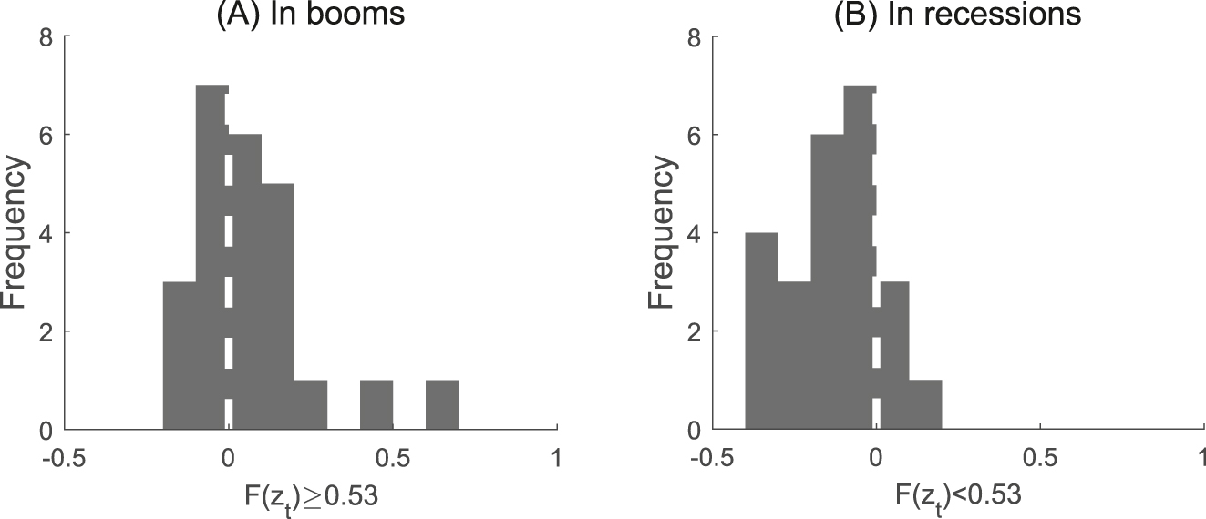
Distribution of output impulse responses. Notes: The histogram in Panel (A) shows the distributions of average responses of industrial productions of 24 manufacturing industries to monetary policy innovations in booms, defined as periods when the smooth logistic function value is greater than 0.53. The histogram in Panel (B) depicts the distributions of average responses of industrial productions of 24 manufacturing industries to monetary policy innovations in recessions, defined as periods when the smooth logistic function value is smaller than 0.53. The responses are cumulated cumulative responses for 36 months after a monetary policy shock.
5.3 Financial Characteristics Indicators
We construct three indicators representing industries’ financial characteristics following Peersman and Smets (2005). The first indicator is the leverage ratio (LEVERAGE), defined as total debt over total assets. The ex-ante relationship between this indicator and balance sheet strength, or the cost of financing external funds, is ambiguous (Dedola and Lippi 2005; Peersman and Smets 2005). A high leverage ratio typically signals a weak balance sheet, as highly leveraged firms face greater repayment pressure. In this case, the external finance premium is expected to increase more in highly leveraged industries in response to monetary policy, leading to a greater contraction in production. However, a high leverage ratio may also indicate a strong ability to repay debt and better access to external financing. If this is the case, highly leveraged firms would be less affected by monetary policy. In this sense, it is necessary to be cautious when interpreting the relationship between this indicator and output responses to monetary policy. The second indicator is the coverage ratio (COVERAGE), defined as operating profits over interest payments. As is the case for the leverage ratio, it is ambiguous whether a higher level of coverage ratio indicates financial strength or weakness. A high coverage ratio could signal a sound cash flow sufficient to cover interest costs, but it might reflect low interest payments indicating weak borrowing capacity. Thus, the relationship between this indicator and output responses to monetary policy is ambiguous, too (Peersman and Smets 2005). The third indicator is the ratio of short-term debt (less than one year) to total debt (STDEBT). A high level of the ratio is a signal of weak balance sheet since it implies that large amounts of debt are nearing repayment or/and the access to long-term funding is restricted. Therefore, sectors with higher short-term debt relative to total debt are expected to exhibit larger declines in production in response to monetary policy.
Panel (A) in Table 2 displays the three financial indicators for 24 manufacturing industries. The figures are derived from firm-level balance sheet information for each industry, covering the period from January 2009 to December 2019. Panel (B) in Table 2 presents the cross-correlations among the indicators. There is a significant negative correlation between the leverage ratio (LEVERAGE) and the coverage ratio (COVERAGE). In contrast, the relationships of the ratio of short-term to total debt (STDEBT) with the other two indicators are not significant.
Indicators of financial conditions in manufacturing industries.
| Panel (A) Financial features by sub-sectors | LEVERAGE | COVERAGE | STDEBT |
|---|---|---|---|
| Industries | |||
| Food products | 0.46 | 5.45 | 0.68 |
| Beverages | 0.46 | 7.37 | 0.62 |
| Tobacco products | 0.25 | 119.80 | 0.89 |
| Textiles, except apparel | 0.49 | 1.93 | 0.70 |
| Wearing apparel, clothing accessories and fur articles | 0.48 | 5.28 | 0.79 |
| Tanning and dressing of leather, luggage and footwear | 0.43 | 9.16 | 0.82 |
| Wood products of wood and cork; except furniture | 0.51 | 2.30 | 0.69 |
| Pulp, paper and paper products | 0.49 | 3.46 | 0.65 |
| Printing and reproduction of recorded media | 0.54 | 2.62 | 0.68 |
| Coke, hard-coal and lignite fuel briquettes and refined petroleum products | 0.55 | 6.65 | 0.64 |
| Chemicals and chemical products | 0.42 | 9.27 | 0.65 |
| Pharmaceuticals, medicinal chemicals and botanical products | 0.37 | 7.05 | 0.68 |
| Rubber and plastic products | 0.49 | 4.49 | 0.69 |
| Other non-metallic mineral products | 0.44 | 5.35 | 0.62 |
| Basic metal products | 0.41 | 4.45 | 0.60 |
| Fabricated metal products, except machinery and furniture | 0.54 | 2.72 | 0.72 |
| Electronic components, computer, and communication equipment | 0.34 | 15.74 | 0.74 |
| Medical, precision and optical instruments, watches and clocks | 0.45 | 6.19 | 0.75 |
| Electrical equipment | 0.48 | 3.42 | 0.72 |
| Other machinery and equipment | 0.55 | 3.67 | 0.72 |
| Motor vehicles, trailers and semitrailers | 0.44 | 6.77 | 0.71 |
| Other transport equipment | 0.67 | 0.75 | 0.74 |
| Furniture | 0.46 | 6.87 | 0.81 |
| Other manufacturing | 0.47 | 4.67 | 0.77 |
| average | 0.47 | 10.23 | 0.71 |
| average (excluding Tobacco products) | 0.47 | 5.46 | 0.70 |
| Panel (B) Correlations | |||
| LEVERAGE (total debt / total assets) | 1 | ||
| (–) | |||
| COVERAGE (operating profits / interest payments) | −0.732*** | 1 | |
| (0.000) | (–) | ||
| STDEBT (short-term debt / total debt) | 0.063 | 0.131 | 1 |
| (0.775) | (0.551) | (–) |
-
Panel (A) presents financial characteristics of 24 manufacturing industries. Industry classification follows the KSIC (Korean standard industrial classification, 9th revision). Panel (B) presents cross-correlation across the indicators of industry characteristics. Tobacco products are excluded from the calculation. P-values are in parentheses. ***: significant at the 1 percent level, **: significant at the 5 percent level, *: significant at the 10 percent level.
5.4 Financial Characteristics and Monetary Policy Effect
In order to examine whether the asymmetric effects of monetary policy across business cycles are related to the financial characteristics, we estimate the simultaneous equation system as follows:
where the subscript i denotes the manufacturing industry, and the superscripts r and b indicate economic recessions and booms, respectively. The dependent variables,
Table 3 shows the results from the estimation of the equation system (4). For comparison, we first estimate a symmetric version of the system as a benchmark case, followed by an estimation that allows for a possible asymmetric impact of financial conditions across business cycles.[9] The coefficient for the leverage ratio (LEVERAGE) is estimated as 0.413 and significant at the 10 percent level under the assumption of symmetric transmission. Although the predicted sign was ambiguous ex-ante, our empirical results show a positive coefficient. This indicates that output decreases to a lesser degree in industries with higher leverage ratios following a monetary policy shock suggesting that highly leveraged firms could be less sensitive to monetary policy on average. This could mean that a high leverage ratio reflects greater borrowing capacity, indicating stronger balance sheet conditions. This effect is more evident in booms rather than in recessions. In booms, the coefficient is estimated as 1.168 and significant at the 5 percent level. In contrast, the coefficient in recessions is estimated statistically insignificant. The difference across business cycles is estimated at 1.512 and significant at the 5 percent level. This result implies that higher leverage, which indicates relatively strong financial conditions, amplifies the asymmetric effects of monetary policy across business cycle phases, which is consistent with previous findings in the literature (Peersman and Smets 2005).
Industry financial characteristics and output impulse responses.
| Linear | Asymmetric responses | |||
|---|---|---|---|---|
| Boom | Recession | Difference | ||
|
|
|
|
||
| LEVERAGE | 0.413* | 1.168** | −0.343 | 1.512** |
| (Total debt / total assets) | (0.090) | (0.014) | (0.351) | (0.027) |
| STDEBT | 0.045 | 0.243 | 0.056 | 0.187 |
| (Short-term debt / total debt) | (0.875) | (0.679) | (0.896) | (0.822) |
| COVERAGE | −0.001 | −0.001 | 0.001 | −0.002 |
| (Operating profits / interest payments) | (0.529) | (0.436) | (0.645) | (0.431) |
-
The figures present the estimation results of Equation (4). P-values are in parentheses. ***: significant at the 1 percent level, **: significant at the 5 percent level, *: significant at the 10 percent level. The estimation results remain effectively the same when Tobacco products are excluded.
For the other two financial indicators, the coverage ratio (COVERAGE) and the short-term debt relative to total debt (STDEBT), we do not find any significant relationship between financial characteristics and the average output responses across business cycle phases.
6 Conclusions
In this paper, we provide empirical evidence demonstrating that the stance of monetary policy – whether tightening or loosening – plays a critical role in its transmission across business cycles, with a focus on Korea in the period following the global financial crisis. The finding that monetary policy exerts a greater influence on output and prices during recessions is not novel, as several prior studies have reported similar outcomes. The traditional interpretation of such findings suggests that monetary policy is an effective instrument for revitalizing a struggling economy, assuming that monetary authorities adopt expansionary policies during recessions.
Our study diverges from previous research by examining the asymmetric effects of monetary policy that may arise not only from economic conditions but also from the stance of the policy itself. We find that contractionary monetary policy significantly impacts a contracting economy, whereas expansionary monetary policy has minimal influence on an expanding economy. The results from our extended experiments are crucial as they suggest the need to reinterpret prior empirical evidence. Specifically, the evidence that monetary policy significantly impacts the economy during downturns does not inherently imply its efficacy as a stabilization tool. In this context, it is essential to reevaluate earlier studies that did not concurrently consider both economic conditions and policy stance as potential sources of asymmetric monetary policy transmission. Monetary authorities should be aware that the effects of their policy implementations across business cycles might manifest differently than previously believed.
Acknowledgment
We are grateful to the journal Editor, Arpad Jeno Abraham, Associate Editor, Anna Rogantini Picco, and two anonymous referees for their helpful comments and suggestions.
Appendices
A Data Sources
Real-time data and economic forecasts: Real-time data and economic forecasts used in the regression for the monetary policy shock identification are collected from the Bank of Korea’s reports, Main Economic Indicators and Economic Outlook. Main Economic Indicators is the bank’s internal report that is prepared for the Monetary Policy Board at policy decision meetings. The report includes information on the real-time data on comprehensive macroeconomic variables, such as GDP and its sub-components, production, prices, and so on. Economic Outlook is the BOK’s official economic forecasts produced and released four times a year. The outlook contains the bank’s quantitative forecasts on economic growth, inflation, the number of employed and unemployment rate, and current accounts in biannual window as well as its qualitative assessment on overall economic conditions. See Lee and Park (2022) for further information on these sources. Macroeconomic variables: Macroeconomic variables used in the estimation are Composite index (Statistics Korea); Industrial Production index (Statistics Korea); Producer Price index (Bank of Korea); Consumer price index (Statistics Korea). Firm-level financial variables in manufacturing industries: KISVALUE (NICE Information Service).
B Results for IP Manufacturing and PPI
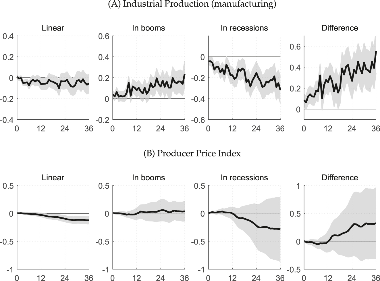
Responses to monetary policy shocks. Notes: The figure plots responses of the industrial production index for manufacturing and producer price index to monetary policy shocks. The responses are generated by estimating Equation (2) using the local projection procedure. Solid lines represent the estimated responses to one unit of monetary policy shocks. X-axis denotes time horizons (months) and Y-axis denotes the magnitude of responses measured in log points. The responses at horizon h are cumulative responses which add up the responses from period 0 to h. Shaded bands represent one-standard confidence intervals generated from 1,000 times bootstrap replications.
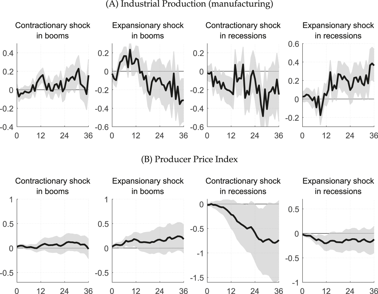
Responses to contractionary and expansionary monetary policy shocks. Notes: The figure plots responses of industrial production index for manufacturing and producer price index to monetary policy shocks. The responses are generated by estimating Equation (3) using the local projection procedure. Solid lines represent the estimated responses to one unit of monetary policy shocks. X-axis denotes time horizons (months) and Y-axis denotes the magnitude of responses measured in log points. The responses at horizon h are cumulative responses which add up the responses from period 0 to h. Shaded bands represent one-standard confidence intervals generated from 1,000 times bootstrap replications
References
Alpanda, Sami, Eleonora Granziera, and Sarah Zubairy. 2021. “State Dependence of Monetary Policy Across Business, Credit and Interest Rate Cycles.” European Economic Review 140: 103936. https://doi.org/10.1016/j.euroecorev.2021.103936.Suche in Google Scholar
Angrist, Joshua D., Òscar Jordà, and Guido M. Kuersteiner. 2018. “Semiparametric Estimates of Monetary Policy Effects: String Theory Revisited.” Journal of Business & Economic Statistics 36 (3): 371–87. https://doi.org/10.1080/07350015.2016.1204919.Suche in Google Scholar
Barnichon, Régis, and Christian Matthes. 2018. “Functional Approximation of Impulse Responses.” Journal of Monetary Economics 99: 41–55. https://doi.org/10.1016/j.jmoneco.2018.04.013.Suche in Google Scholar
Barnichon, Régis, Christian Matthes, and Sablik Timothy. 2017. “Are the Effects of Monetary Policy Asymmetric?” Economic Brief 17 (3).Suche in Google Scholar
Bernanke, Ben S., and Mark Gertler. 1995. “Inside the Black Box: The Credit Channel of Monetary Policy Transmission.” Journal of Economic Perspectives 9 (4): 27–48. https://doi.org/10.1257/jep.9.4.27.Suche in Google Scholar
Cloyne, James, and Patrick Hürtgen. 2016. “The Macroeconomic Effects of Monetary Policy: A New Measure for the United Kingdom.” American Economic Journal: Macroeconomics 8 (4): 75–102. https://doi.org/10.1257/mac.20150093.Suche in Google Scholar
Cover, James Peery. 1992. “Asymmetric Effects of Positive and Negative Money-Supply Shocks.” The Quarterly Journal of Economics 107 (4): 1261–82. https://doi.org/10.2307/2118388.Suche in Google Scholar
De Long, J. Bradford, Lawrence H. Summers, N. Gregory Mankiw, and Christina D. Romer. 1988. “How Does Macroeconomic Policy Affect Output?” Brookings Papers on Economic Activity 1988 (2): 433–94. https://doi.org/10.2307/2534535.Suche in Google Scholar
Debortoli, Davide, Mario Forni, Luca Gambetti, and Luca Sala. 2020. “Asymmetric Effects of Monetary Policy Easing and Tightening.” CEPR Discussion Paper No. DP15005.Suche in Google Scholar
Dedola, Luca, and Francesco Lippi. 2005. “The Monetary Transmission Mechanism: Evidence from the Industries of Five OECD Countries.” European Economic Review 49 (6): 1543–69. https://doi.org/10.1016/j.euroecorev.2003.11.006.Suche in Google Scholar
Garcia, René, and Huntley Schaller. 2002. “Are the Effects of Monetary Policy Asymmetric?” Economic Inquiry 40 (1): 102–19. https://doi.org/10.1093/ei/40.1.102.Suche in Google Scholar
Gonçalves, Sílvia, Ana María Herrera, Lutz Kilian, and Elena Pesavento. 2024. “State-dependent Local Projections.” Journal of Econometrics 244 (2): 105702, https://doi.org/10.1016/j.jeconom.2024.105702.Suche in Google Scholar
Granger, Clive W. J., and Timo Terasvirta. 1993. Modelling Non-Linear Economic Relationships. Oxford University Press.Suche in Google Scholar
Hang, Yin, and Wenjun Xue. 2020. “The Asymmetric Effects of Monetary Policy on the Business Cycle: Evidence from the Panel Smoothed Quantile Regression Model.” Economics Letters 195 (C): 109450, https://doi.org/10.1016/j.econlet.2020.109450.Suche in Google Scholar
Jordà, Òscar. 2005. “Estimation and Inference of Impulse Responses by Local Projections.” American Economic Review 95 (1): 161–82. https://doi.org/10.1257/0002828053828518.Suche in Google Scholar
Jordà, Òscar, Sanjay R. Singh, and Alan M. Taylor. 2020. The Long-Run Effects of Monetary Policy. Working Paper Series 2020-01. Federal Reserve Bank of San Francisco.10.24148/wp2020-01Suche in Google Scholar
Karras, Georgios. 1996a. “Are the Output Effects of Monetary Policy Asymmetric? Evidence from a Sample of European Countries.” Oxford Bulletin of Economics and Statistics 58 (2): 267–78. https://doi.org/10.1111/j.1468-0084.1996.mp58002004.x.Suche in Google Scholar
Karras, Georgios. 1996b. “Why Are the Effects of Money-Supply Shocks Asymmetric? Convex Aggregate Supply or “Pushing on a String”?” Journal of Macroeconomics 18 (4): 605–19. https://doi.org/10.1016/s0164-0704(96)80054-1.Suche in Google Scholar
Karras, Georgios, and Houston H. Stokes. 1999. “Why Are the Effects of Money-Supply Shocks Asymmetric? Evidence from Prices, Consumption, and Investment.” Journal of Macroeconomics 21 (4): 713–27. https://doi.org/10.1016/s0164-0704(99)80003-2.Suche in Google Scholar
Lee, Seungyoon, and Jongwook Park. 2022. “Identifying Monetary Policy Shocks Using Economic Forecasts in Korea.” Economic Modelling 111: 1–11. https://doi.org/10.1016/j.econmod.2022.105803.Suche in Google Scholar
Lo, Ming Chien, and Jeremy Piger. 2005. “Is the Response of Output to Monetary Policy Asymmetric? Evidence from a Regime-Switching Coefficients Model.” Journal of Money, Credit, and Banking 37 (5): 865–86. https://doi.org/10.1353/mcb.2005.0054.Suche in Google Scholar
Morgan, Donald P. 1993. “Asymmetric Effects of Monetary Policy.” Economic Review (Q II): 21–33.Suche in Google Scholar
Peersman, Gert, and Frank Smets. 2001. “Are the Effects of Monetary Policy in the Euro Area Greater in Recessions Than in Booms?” European Central Bank Working Paper 52: 65–89.10.2139/ssrn.356041Suche in Google Scholar
Peersman, Gert, and Frank Smets. 2005. “The Industry Effects of Monetary Policy in the Euro Area.” The Economic Journal 115 (503): 319–42. https://doi.org/10.1111/j.1468-0297.2005.00991.x.Suche in Google Scholar
Ravn, Morten O., and Martin Sola. 2004. “Asymmetric Effects of Monetary Policy in the United States.” Federal Reserve Bank of St. Louis Review 86: 41–60. https://doi.org/10.20955/r.86.41.Suche in Google Scholar
Romer, Christina D., and David H. Romer. 2004. “A New Measure of Monetary Shocks: Derivation and Implications.” American Economic Review 94 (4): 1055–84. https://doi.org/10.1257/0002828042002651.Suche in Google Scholar
Tenreyro, Silvana, and Gregory Thwaites. 2016. “Pushing on a String: US Monetary Policy Is Less Powerful in Recessions.” American Economic Journal: Macroeconomics 8 (4): 43–74. https://doi.org/10.1257/mac.20150016.Suche in Google Scholar
Weise, Charles L. 1999. “The Asymmetric Effects of Monetary Policy: A Nonlinear Vector Autoregression Approach.” Journal of Money, Credit, and Banking 31 (1): 85–108. https://doi.org/10.2307/2601141.Suche in Google Scholar
Supplementary Material
This article contains supplementary material (https://doi.org/10.1515/bejm-2024-0127).
© 2025 the author(s), published by De Gruyter, Berlin/Boston
This work is licensed under the Creative Commons Attribution 4.0 International License.
Artikel in diesem Heft
- Frontmatter
- Advances
- Real Wage Cyclicality and Monetary Policy
- Green Transition, Skills Heterogeneity, and Inequality
- Workforce Aging, Growth and Productivity
- Monetary Policy Shocks: Data or Methods?
- Contributions
- Monetary Policy and Labor Market Friction in a HANK Model
- Capital Market Liberalization and Bank Credit Decisions: A Quasi-Natural Experiment Based on the “Mainland-Hong Kong Stock Connect”
- Automation, Skill Premium, and Labor Share
- Business Cycles, Monetary Policy Stance, and Monetary Policy Transmission in Korea
- Forecasting Revisions to U.S. Jobs Report Data
- Loan Loss Provision, Unsecured-Collateralized Loan Choice and Macro-Stability in China
- Price Stickiness, Input–Output Linkages, and Monetary Policy Transmission in Korea
- Oil Price-Driven Inflation and the Channels of Pass-Through
- Firm Dynamics, Informality, and Monetary Policy