
Green Transition, Skills Heterogeneity, and Inequality
-
Marina Albanese


Abstract
This study investigates the labor market dynamics and distributional consequences of the transition to a net-zero economy, with a particular focus on heterogeneity across worker types differentiated by skill level and sectoral employment. We employ a Dynamic Stochastic General Equilibrium (DSGE) model with search-and-matching (SAM) frictions in the labor market, incorporating three dimensions of heterogeneity: (i) differentiation between low-skilled and high-skilled workers; (ii) distinctions among employed, unemployed, and inactive individuals; and (iii) employment distributions across green and dirty sectors. Our main findings are threefold. First, in the short term, the adjustment to higher carbon taxes leads to a reduction in employment and a decline in skill wage premiums. Second, the green transition intensifies inequality in the long run by favoring high-skilled workers, assuming the share of low-skilled labor in the green sector remains persistently limited. Third, we assess the effectiveness of different carbon revenue recycling schemes, including progressive and uniform labor tax cuts and unemployment benefits. We find that aggregate welfare gains are higher when revenues are used to cut labor income taxes for low-skilled workers, and that unemployment benefits generate greater welfare gains than a uniform labor tax cut in the medium to long run.
1 Introduction
The issue of climate change and the transition to a net zero economy is currently one of the most pressing policy concerns. The next decade is poised to witness a rapid escalation of the green transition, which will catalyze notable structural transformations within the labor market (Vandeplas et al. 2022). Hence, to fully understand the implications of green growth on the labor market, a thorough understanding of qualitative changes in the organization and content of workforce is necessary (Consoli et al. 2016). Inevitably, the transition towards a zero-emission economy will result in significant distributional effects (OECD 2023; Ranieri 2013). The question of whether the green transition will drive more job polarization and increase inequalities remains unanswered (OECD 2023). Addressing these issues requires a comprehensive general equilibrium analysis that can incorporate the complexities of search-and-matching frictions in both dirty and green sectors (Hagedorn et al. 2016; Hafstead and Williams 2018). However, existing dynamic general equilibrium models predominantly focus on the short-term effects of environmental regulation (see, e.g., Fischer and Springborn 2011; Heutel 2012; Annicchiarico and Di Dio 2015), with a limited examination of long-term consequences (Ferrari and Nispi Landi 2023; Diluiso et al. 2021; Benmir and Roman 2020).
We contribute to this literature by investigating the following research questions: (i) What are the quantitative impacts of the transition towards a net-zero economy on labor markets and skill requirements? (ii) What are the distributional consequences of transitioning to a net-zero economy? (iii) How can carbon revenue recycling policies be effectively utilized to address the inequalities that may emerge from the green transition? We extend the model to account for heterogeneity along three key dimensions. First, in contrast to existing studies, we differentiate among three types of households: entrepreneurs, high-skilled workers, and low-skilled workers. Second, we distinguish between employed and unemployed statuses within the labor market. Third, we differentiate employment between the green and polluting sectors. Our model includes two perfectly competitive intermediate goods firms, classified as green and polluting, which produce a homogeneous output. These firms rent capital from entrepreneurs and employ both high-skilled and low-skilled labor, with hiring and firing subject to SAM frictions and wages determined through Nash bargaining. By explicitly considering these important market features, our framework allows for a more comprehensive assessment of the labor market and macroeconomic effects of carbon taxes and relative distributional implications.
Our paper makes four significant contributions to this literature. First, to the best of our knowledge, we are the first to examine a dynamic transition toward a net-zero economy considering skill heterogeneity and search-and-matching frictions in a two-sector model accounting for both green and dirty firms. These model characteristics enable a detailed analysis of the implications of a gradual increase in a carbon tax on the labor market and allow for non-perfect substitution of heterogeneous labor between polluting and non-polluting sectors. Second, the presence of heterogeneity allows us to analyze the distributional effects of a green transition in terms of welfare, skill-wage premiums, and consumption inequalities. Third, our analysis considers alternative carbon revenue recycling scheme scenarios aimed at reducing inequalities during the transition toward a net-zero economy. The examination of alternative applications of climate policy revenues enables us to enhance the discourse surrounding the distributional impacts of climate policies. Finally, unlike prior research in this area (e.g., CEDEFOP 2021; OECD 2023), this study investigates the impact of structural changes in productive technology within the green sector. Specifically, it analyzes the macroeconomic implications associated with an increase in the proportion of low-skilled workers within this sector during the green transition.
The main results of our model, calibrated to the Euro Area (EA), can be summarized as follows. At the aggregate level, the gradual implementation of a carbon tax generates a temporary contraction in key macroeconomic indicators, including output, consumption, and investment. Employment initially declines but recovers over time, ultimately increasing by approximately 1.5 % relative to its pre-transition level. The transition induces a structural reallocation of production from the polluting to the green sector. Accounting for skill heterogeneity attenuates the negative impact on aggregate unemployment and output and expedites the shift toward green production. The coexistence of workers with different skill levels and bargaining power enhances labor market adaptability, facilitating sectoral reallocation and reducing adjustment costs. These differences also yield heterogeneous labor market outcomes: in the short run, the green sector absorbs more low-skilled workers, owing to their lower vacancy posting costs. Over time, however, the expansion of green job opportunities becomes increasingly skewed toward high-skilled positions. Although unemployment falls during the initial stages of the transition, participation rates temporarily decline, largely reflecting sharp employment losses in the polluting sector. In the long run, participation recovers, offsetting the adverse income effects of the transition. The transition to a net-zero economy has important distributional implications. While the skill wage premium falls initially, it rises in the long run, widening the consumption gap and reinforcing labor market inequalities. These effects critically depend on the assumption that the green sector maintains a persistently low share of low-skilled labor.
Moreover, we compare three fiscal recycling strategies for carbon tax revenues: progressive labor tax cuts for low-skilled workers, uniform tax cuts for all workers, and unemployment benefits. Progressive tax cuts most effectively reduce wage and consumption inequalities. Unemployment benefits moderately curb consumption inequality and are especially effective in containing the skill premium in the short to medium term. In terms of welfare, targeted tax cuts yield the highest aggregate gains, while unemployment benefits outperform uniform cuts over the medium run. Further analysis of the model stresses the role of structural transformations within the green sector by simulating an increase in the share of low-skilled workers in productive activities. The removal of asymmetries between sectors and workers helps lower transition costs for low-skilled workers, who are disproportionately affected by the shift to a net-zero economy our results suggest that these adjustments in workforce composition can contribute to a fairer transition by mitigating the increase in skill wage premiums and reducing consumption inequality.
The remainder of the paper is organized as follows. Section 2 provides a review of the literature of empirical findings related to environmental policies and the labor market, as well as environmental DSGE models with a focus on the labor market. Section 3 describes the model. Section 4 details the calibration procedure. Section 5 presents the main findings of the research and provides a comprehensive discussion of the fiscal policy implications and structural change in the green sector. Section 6 conducts a welfare analysis. Section 7 provides a sensitivity analysis. Section 8 concludes by summarizing the significant contributions of the study and highlighting avenues for future research.
2 Background
2.1 Green Transition and the Labor Market
The aggregate impact of environmental policies, particularly carbon taxes, on labor demand remains a contentious and largely unresolved empirical issue. The literature reveals mixed findings, especially when differentiating between high-cost polluting industries and broader macroeconomic perspectives. Several studies focusing on high-pollution industries generally report negative employment impacts due to stringent environmental regulations. For instance, Greenstone (2002), Kahn and Mansur (2013), Walker (2011) document adverse employment effects in these sectors. In contrast, the broader macroeconomic literature often finds positive correlations between green innovation policies and employment. Horbach and Rennings (2013) and Gagliardi et al. (2016) suggest that policies promoting green technologies tend to enhance employment. Despite ongoing policy debates on green jobs and skills, empirical studies on the skill bias of environmental policies remain scant and predominantly US-centric (Marin and Vona 2019). Notably, Elliott and Lindley (2017) found that plants producing green goods and services employ fewer production workers, based on the US Green Goods and Services Survey for 2010 and 2011. Similarly, Consoli et al. (2016) and Bowen et al. (2018) found modest skill differences between green and non-green jobs but noted a bias towards higher skills for green jobs. Vona et al. (2018) tested the effect of amendments to the Clean Air Act on skill demand in US regions from 2006 to 2014, finding significant skill gaps, especially in engineering and technical skills.
Based on these findings, climate policies are anticipated to drive long-term skill upgrade, particularly in engineering and technical fields. Chen et al. (2020) and Vona (2023) emphasize addressing the skill mismatch between green job requirements and the existing workforce’s capabilities. Studies consistently show that green jobs demand a diverse range of skills at various proficiency levels, from medium to high (Marin and Vona 2019; Saussay et al. 2022; Vona 2023), and underscore the importance of on-the-job training (Consoli et al. 2016; Popp et al. 2020, 2022; Vona 2023). Effective training programs are crucial for facilitating workers’ transition to green jobs and mitigating economic displacement. Given that skills can depreciate during job transitions (Gathmann and Schönberg 2010), the associated costs and wage differentials depend significantly on how easily workers can be retrained for green skills, underscoring their specificity (Vona 2023).
Recent research indicates that the skills sets required for green jobs are more aligned with those needed in carbon-intensive sectors compared to other occupations, suggesting that workers displaced from these sectors can be effectively reemployed in green jobs (Popp et al. 2022; Saussay et al. 2022; Vona et al. 2018). Nevertheless, the OECD (2023) notes a potential shift toward medium- and low-skilled occupations in future green jobs, implying a reduction in job polarization. Employment growth is projected to be higher in skilled manual and elementary occupations than in high-skilled ones. The demand for high-level skills due to ICT adoption has decelerated over the past decade, possibly due to the technology’s maturation (Vona et al. 2015). Furthermore, unemployed workers are more likely to transition to green jobs than high-polluting ones, especially in countries with high overall job-finding rates (OECD 2023).
2.2 E-DSGE and the Labor Market
The impact of the green transition on the labor market has received limited attention in the DSGE literature. Few papers simultaneously analyze environmental regulations and the labor market. Among others, Hafstead and Williams (2018) examine the effects of environmental policy on employment and unemployment using a new general equilibrium two-sector search model. They include search-and-matching frictions in dirty and green sectors but do not consider skill heterogeneity. Similarly, Aubert and Chiroleu-Assouline (2019) construct a general equilibrium model incorporating heterogeneous workers, imperfect labor markets (search and match), and externalities of pollution consumption. However, their model considers both high-skilled and low-skilled workers, with unemployment only applying to low-skilled workers. Moreover, the model does not explicitly distinguish between clean and dirty sectors. Castellanos and Heutel (2019) develop a static computable general equilibrium model of the US economy to examine the unemployment effects of climate policy and the significance of cross-industry labor mobility. Shapiro and Metcalf (2023) explore the impact of endogenous labor force participation on labor markets in a model that examines firm creation and the adoption of green production technologies. Gibson and Heutel (2023) explore the relationship between unemployment and the business cycle in the presence of environmental regulation. Nevertheless, current dynamic general equilibrium models fall short of incorporating skill heterogeneity in the transition toward a net zero economy.
These findings underscore the critical importance of accounting for skills heterogeneity when analyzing the inequality implications of a green transition. Ignoring these characteristics of the labor market could lead to misguided policy recommendations. Consequently, the next section introduces a novel E-DSGE model, designed to examine the distributional effects of environmental policies across various types of workers.
3 The Model
The model presented in this section is a New Keynesian E-DSGE model that incorporates search-and-matching (SAM) frictions in the labor market as in Mortensen and Pissarides (1994) and Monacelli et al. (2010). Our model extends this framework to capture population heterogeneity in three dimensions. First, following Dolado et al. (2021), we consider three distinct households: entrepreneurs, and high-skilled and low-skilled workers. Second, we distinguish between two labor market statuses: employed and unemployed. Third, we differentiate the employment status within the labor market, specifically between the green and dirty sectors. The green sector generates output without carbon emissions, while the dirty sector produces output through a polluting process. However, firms in the dirty sector decide on their abatement spending to limit emissions and thereby reduce carbon tax expenses. Both green and brown outputs serve as inputs for a continuum of intermediate firms operating in monopolistic competition. A final-good firm then combines these differentiated intermediate goods to produce a final product. These firms rent capital from entrepreneurs and employ high- and low-skilled labor from workers. Hiring and firing are subject to SAM frictions, and wages are set by Nash bargaining.
3.1 Labor Market and Matching Process
The model presents three different types of households: high-skilled workers, low-skilled workers, and entrepreneurs, each with a constant mass indicated by φ
s
, where s ∈ {H, L, E}.[1] Similarly, we define j ∈ {D, G} as the sector type, where G represents the green sector and D represents the dirty sector. At any given time, an individual, irrespective of their type, can be in one of three distinct labor market statuses: employed in a green firm
The number of newly employed workers
where
These assumptions imply that the probability for a vacancy to be filled is the following:
where
denotes labor market tightness for s type of households and the j sector.
Similarly, the probability of finding a job is given by:
The timing is as follows. In a given period t, firm j starts with an employment level of
The model takes into account two major channels in which labor market conditions interact endogenously with other macroeconomic sectors. One is the participation choice of the household through
In detail, each worker chooses their participation in the labor force and decides whether to start searching for a job. However, this process is constrained by search and matching frictions. As a result, each household can only determine their employment status for the next period within the limitations imposed by these frictions. Consequently, employment in each sector and for each type of worker becomes a state variable, predetermined by previous labor market conditions. Notably, due to the time endowment constraint, once employment and unemployment are accounted for, leisure becomes merely a residual variable. Thus, the participation margin today can only be adjusted by opting for unemployment. The choice of
3.2 Households
The model incorporates three categories of households: high-skilled workers, low-skilled workers, and entrepreneurs.
3.2.1 Entrepreneurs Households
In line with Dolado et al. (2021), entrepreneurs do not participate in the labor market. However, entrepreneurs invest in physical capital in both sectors (k
j,t
), in a risk-free bond
subject to:
where
The first-order conditions with respect to consumption, the risk-free bond, investment and capital in the dirty and green sectors are as follows:
where
3.2.2 High and Low Skilled Workers
In order to model the workers’ choices, we use the model setup proposed by Dolado et al. (2021). Workers of each type maximize their utility, subject to both the budget constraint and employment flow constraints due to search and matching (SAM) frictions. The optimization problem for workers of type s ∈ {H, L} can be formulated as follows:
subject to a single period-by-period budget constraint, as in the following:
and the law of motion of employment in the green and dirty sectors:
where ψ
s
represents the elasticity of labor supply, and ϕ
s
is the weight of leisure for each type of household, and h
s
is the consumption habits parameter. Both households can invest in a risk-free bond
The first-order conditions with respect to consumption, the risk-free bond, unemployment and green and dirty employment are as follows:
where
3.3 Production Sector
3.3.1 Final Good Firms
The representative final good firm uses the following CES bundle to produce the total production
3.3.2 Intermediate-Good Firms
There is a continuum of firms indexed by i, producing a differentiated input and using the following production function:
where
where ξ defines the elasticity of substitution between dirty and green goods. Firms operate in monopolistic competition and set prices subject to the demand of the final-good firm. Firms pay quadratic adjustment costs à la Rotemberg
where
The intermediate firm i solves an intratemporal problem to choose the optimal input combination and an intertemporal problem to set the price. The intratemporal problem, i.e., minimizing costs subject to a given level of production, yields the following demand functions for the green and dirty input:
where p G,t and p D,t are the prices of green and dirty production, respectively, expressed relative to the CPI; p I,t represents the real marginal cost of the firm:
Formally, the firm sets the price p
I,t
by maximizing the present discounted value of profits subject to the demand constraint
where λ t represents the aggregate marginal utility of consumption. Equation (28) links inflation to real marginal costs. If γ p > 0, changing prices is costly, and the classical dichotomy between nominal and real variables does not hold.
3.4 Green and Dirty Firms
The economy comprises two distinct sectors: the “Green” sector and the “Dirty” sector. Within each sector, intermediate firms generate output utilizing two different technological approaches. Firms in the green sector adopt sustainable production processes, predominantly relying on renewable resources and emitting minimal carbon dioxide. Conversely, firms in the Dirty sector employ pollutant technologies, such as fossil fuels, resulting in high carbon emissions. These firms are referred to as Carbon-Intensive firms. Following Giovanardi et al. (2021) and Ferrari and Nispi Landi (2023), we incorporate the complementarity between capital and energy. Specifically, we assume that green capital is complementary to renewable energy, whereas dirty capital is complementary to fossil fuel energy.
3.4.1 Dirty Firms
Intermediate dirty firms produce output by employing capital, skilled labor, and unskilled labor according to the following technology function.
Following the approach of Sun et al. (2023), we employ a Cobb-Douglas production function characterized by the following parameters: α
D
representing the capital share,
The production activities in the so-called “dirty sector” generate pollutants emissions. Empirical observations suggest that emissions at the level of dirty firms, denoted by em t , exhibit a proportional relationship with the level of output generated by the same firms. Furthermore, it is possible for such firms to mitigate their emissions by investing in abatement activities pertaining to clean technology. The emission function reads as follows:
where φ determines the emission intensity and μ t is the abatement effort. Nevertheless, the abatement activity is costly. Following Nordhaus (2008) and Ferrari and Nispi Landi (2023), we assume a convex abatement-cost function:
where φ 1 and φ 2 are technological parameters. The stock of atmospheric carbon m t accumulates following this law of motion:
where δ m represents the emission decay rate. Following the methodology proposed by Annicchiarico and Di Dio (2015).
The dirty firms maximize the following profit function with respect to capital, employment, vacancies for both types of households, and abatement effort:
where
The first order conditions for dirty firms with respect to capital, high-skilled employment, low-skilled employment, high-skilled vacancies, low-skilled vacancies and abatement effort are:
where
3.4.2 Green Firms
The intermediate green firms produce output by employing capital, skilled labor, and unskilled labor according to the following technology function:
where α
G
is the share of capital in the production process,
Green firms maximize the following profit function with respect to capital, employment, and vacancies for both types of households:
where
where
3.5 Wage Setting
The wage is determined through a Nash bargaining process in each sector and for each type of worker, where
where
The solution of this maximization problem provides the real wage determination for low- and high-skilled workers across both the dirty and green sectors:
3.6 Government
Government revenue is represented by carbon tax revenues. Fiscal policy involves public spending, unemployment benefits and labor income taxes. The government runs a balanced budget in every period:
Public spending in the government (g t ) is fixed as a constant proportion of total output.
The Nominal Interest rate follows a Taylor rule:
where y t is the aggregate output and y ss and π ss , denote the deterministic steady-state of the nominal interest rate inflation rate and aggregate output; ι r is the monetary policy inertia parameter; ι π is the coefficient on inflation in the feedback rule and ι y is the coefficient on output.
3.7 Market Clearing and Aggregations
Combining the budget constraints of the households and the government and using the bonds market clearing condition we obtain the following market clearing condition in the good sector:
where c
t
is the aggregate consumption and is equal to the sum of consumption for each type of family weighted by their share:
3.8 Inequality Measures
To conduct a specific analysis of inequality along the green transition, we consider the following measures of inequality across households:
Equation (58) represents the aggregate wage premium for high-skilled workers over low-skilled workers (aggregate skill premium). Equations (59) and (60) define the skill premium in the green and dirty sectors, respectively. In addition, we employ three measures of inequality based on consumption. Equation (61) denotes the consumption inequality between high-skilled and low-skilled workers. Equations (62) and (63) define the consumption inequality between entrepreneurs and low-skilled workers and between entrepreneurs and high-skilled workers, respectively.
4 Calibration
The model is calibrated for the euro area at a quarterly frequency to ensure comparability with existing theoretical models on green transition. See Table 1 for the complete description of model calibration. Parameters are selected to capture the principal structural characteristics of the euro area and chosen based on standard values found in the literature. These parameters are calibrated to align with targets concerning steady-state unemployment rate values, distinguished between high- and low-skill labor markets. Specifically, these targets correspond to the participation and unemployment rates for both categories of workers, as described below.
4.1 Labor Market and Demographics
Labor market parameters are calibrated to reflect the participation and unemployment rates for high-skilled and low-skilled workers within the Euro area. The skill-specific unemployment rates are set based on the average values observed during the sample period of 2021–2024. Following Eurostat data, these rates are 4.3 % for high-skilled workers and 12 % for low-skilled workers.[3] The labor force participation rate in the Euro area, for the same sample period, is 65 % for high-skilled workers and 63 % for low-skilled workers.[4] The share of entrepreneur (φ E ) is set equal to 0.10 according to Abbritti and Consolo (2022). The relative mass of the high-skilled household is set to match the share of the employed population with tertiary education as reported in Eurostat.[5] In the Euro Area, the population aged 15–64 the average share of high-skilled individuals (those with tertiary education) is 31 %, while the average share of low-skilled individuals (those with less than primary, primary, lower secondary, upper secondary, and post-secondary non-tertiary education) is 69 %.[6] Following this classification, in our model, 28 per cent of households are set as high-skilled workers (φ H ) and 62 per cent as low-skilled workers (φ L ).
According to Dolado et al. (2021), the matching efficiency parameter is set differently between workers, with a higher value of 0.72 for high-skilled workers
Furthermore, since there are unequal shares of different skill types in the population, in addition to our skill-specific steady-state targets for employment variables, this results in further asymmetries for calibration parameters. Taking into account the lower participation rate of low-skilled workers, leisure (inactivity) will be a greater contribution to the utility function (ϕ
L
> ϕ
H
). To calibrate bargaining power parameters, we follow the same approach as Gibson and Heutel (2023), by setting these values to match labor market-specific features. Some other studies simply assume symmetric bargaining (
4.2 Households
The benchmark for households parameters have been set in accordance with the existing literature. The discount factor (β
s
) has been assigned a value of 0.99; the elasticity of the labor supply
4.3 Production
The calibration of key parameters for the production sector has been carried out relying on the New Area-Wide Model (NAWM-II) of Coenen et al. (2018) and Ferrari and Nispi Landi (2023). Among these, the elasticity of substitution between differentiated goods (ɛ) has been fixed at 3.85; the share of capital in production (α j ) has been assigned a value of 0.33; and the quarterly depreciation rate of capital has been set to 2.5 %. The allocation of high-skilled and low-skilled workers in the production function is determined based on OECD (2023) data regarding the proportion of green-task versus nongreen-task jobs by the educational attainment of workers. Consequently, we assign 55.5 % of workers in the green sector as high-skilled and 46.6 % in the dirty sector. The investment adjustment costs have been determined to be equal to 10.78.
In order to set the weight of the dirty output and the elasticity of substitution between the green and the dirty outputs, we follow Giovanardi et al. (2021), Carattini et al. (2021), and Ferrari and Nispi Landi (2023). In particular, we consider these two productive sectors different in the energy sources, with a relatively high elasticity of substitution. According to Carattini et al. (2021), a value of 2 is assigned to the substitutability parameter between dirty and green goods (ξ). However, Giovanardi et al. (2021) provide a weight of 0.8 for the dirty good, based on the share of renewable energy in Europe in 2018. The specific technologies in both the green and dirty sectors are calibrated to match the aforementioned parameters. Consequently, the technology available in the dirty sector is found to be more efficient than that in the green sector, such that A G < A D .
4.4 Environmental Sector
In terms of environmental parameters, we adopt the calibration approach presented by Gibson and Heutel (2023). Specifically, we set the pollution decay rate, denoted δ m , at 0.0035 (which implies a yearly depreciation rate of 1.5 %). The convexity parameter, denoted as φ 2, in the abatement function is calibrated at 1.6. The coefficient in the abatement function, φ 1, is established as 0.1924, as reported in Ferrari and Nispi Landi (2023). The coefficient in the emission function, denoted φ, is set at 0.45, following the results reported by Annicchiarico and Di Dio (2015).
4.5 Policies
The Taylor rule parameters are calibrated based on the specifications of the NAWM-II model as follows: ι
π
= 2.74, ι
y
= 0, and ι
r
= 0.93. Public spending as a fraction of GDP is set at 0.21, following Ferrari and Nispi Landi (2023). To focus on the implications of the green transition on the labor market, in the baseline calibration, we exclude the recycling of carbon tax revenues and set
Parameters and selected steady-state values.
| Calibrated parameters | |||||
| Efficiency of matching, H |
|
0.72 | Elas. of subst. dirty-green good | ξ | 2.00 |
| Efficiency of matching, L |
|
0.46 | Elas. of subst. differentiated goods | ɛ | 3.58 |
| Elasticity of matches, H |
|
0.60 | Green sector size | γ | 0.20 |
| Elasticity of matches, L |
|
0.40 | Capital share in the production function | α j | 0.33 |
| Separation rate, high-skilled |
|
0.03 | High-skilled share production function, G |
|
0.36 |
| Separation rate, low-skilled |
|
0.06 | High-skilled share production function, D |
|
0.23 |
| Share of entrepreneur | φ E | 0.10 | Vacancy posting costs |
|
0.13 |
| Share of high-skilled | φ H | 0.28 | Adjustment costs on investments |
|
10.47 |
| Share of low-skilled | φ L | 0.62 | Emission by product from dirty output | φ | 0.45 |
| Risk aversion | σ s | 2.00 | Abatement cost parameter | φ 1 | 0.19 |
| Discount factor | β s | 0.99 | Abatement cost parameter | φ 2 | 1.60 |
| Labor supply elasticity | ψ s | 1.00 | Decay rate of carbon emissions | δ m | 0.0035 |
| Targeted steady states | Parameters targeting steady state | ||||
| Participation rate, H | par H | 0.65 | Utility weight of leisure, H | ϕ H | 1.92 |
| Participation rate, L | par L | 0.63 | Utility weight of leisure, L | ϕ L | 6.21 |
| Unemployment rate, H | un H | 0.04 | Bargaining power dirty sector, H |
|
0.03 |
| Unemployment rate, L | un L | 0.12 | Bargaining power dirty sector, L |
|
0.03 |
| Non targeted steady states | Bargaining power green sector, H |
|
0.86 | ||
| Job-finding rate, H | f H | 0.48 | Bargaining power green sector, L |
|
0.73 |
| Job-finding rate, L | f L | 0.22 | Total factor productivity dirty |
|
1.72 |
| Total factor productivity green |
|
0.75 | |||
| Inequality measures | |||||
| Wage premium | 2.51 | Inequality, HL | 2.83 | ||
| Wage premium, green sector | 2.51 | Inequality, EL | 11.69 | ||
| Wage premium, dirty sector | 2.51 | Inequality, EH | 4.13 | ||
5 Results
The European Union aims to achieve climate neutrality by 2050, striving for an economy with net-zero greenhouse gas emissions (European Commission 2019). To explore this transition, we simulate a pathway toward a net-zero economy. Our analysis begins in period 0, corresponding to the fourth quarter of 2019, with the introduction of a government emissions tax that increases linearly over 30 years, targeting zero emissions by 2050. Starting from a baseline calibration without environmental policy (τ = 0), we investigate the effects of an incremental increase in τ, designed to reduce long-term emissions by 100 % over 30 years (120 quarters). We solve the model under the assumption of perfect foresight.[7]
5.1 Transitional Dynamics to a Green Economy
In this section, we examine the transitional dynamics of key macroeconomic variables and measures of inequality. Figure 1 shows the dynamics of the carbon tax and carbon emissions (solid black line). Period 0 corresponds to the fourth quarter of 2019, when the government introduces an emissions tax that increases linearly over 120 quarters, leading to complete reduction in emissions by 2050.[8]
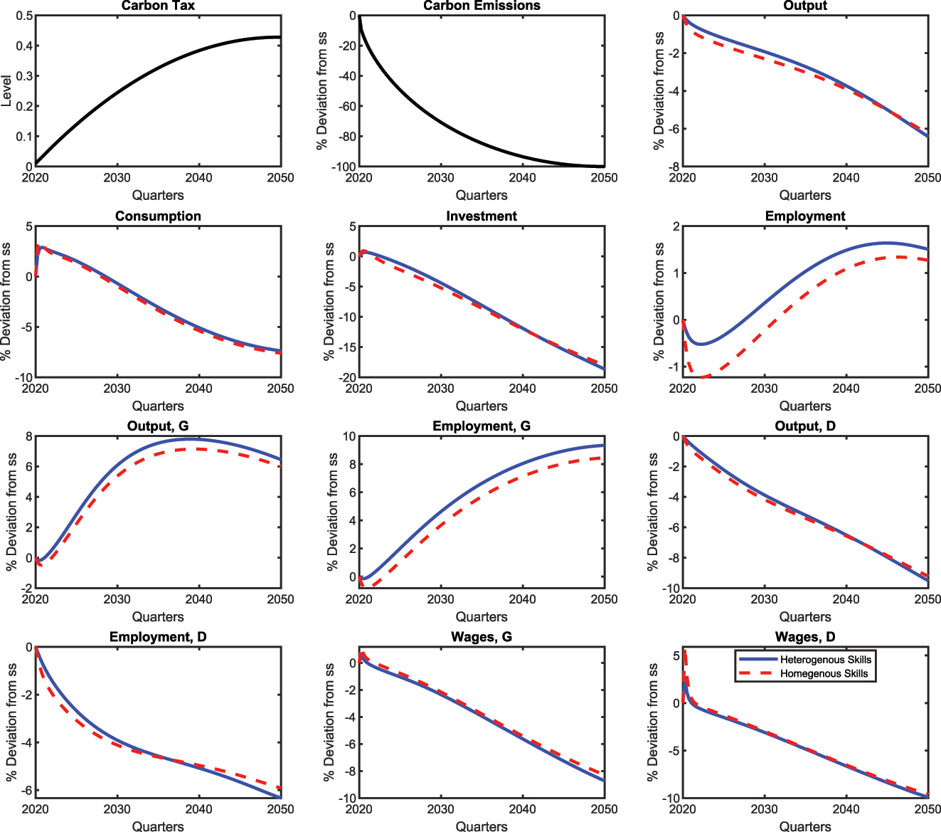
Transition to a net-zero economy: Policy and aggregate variables. Note: The blue line represents the SAM model with worker heterogeneity (i.e., low- and high-skilled workers), while the dotted red line represents the model without household heterogeneity. The black line represents the trajectory of policy and emissions dynamics.
To highlight the relevance of our findings we compare our results to those of a simpler DSGE model that abstracts from skills heterogeneity. Figure 1 presents the transition of the selected variables in response to the gradual increase in carbon taxes by considering (i) a SAM model with low and high-skilled workers (solid blue line) and (ii) a SAM model that does not account for worker heterogeneity (dotted red line).[9] Figure 2 illustrates the transition in the labor market for heterogeneous households. Figure 3 displays the inequality implications of a green transition.
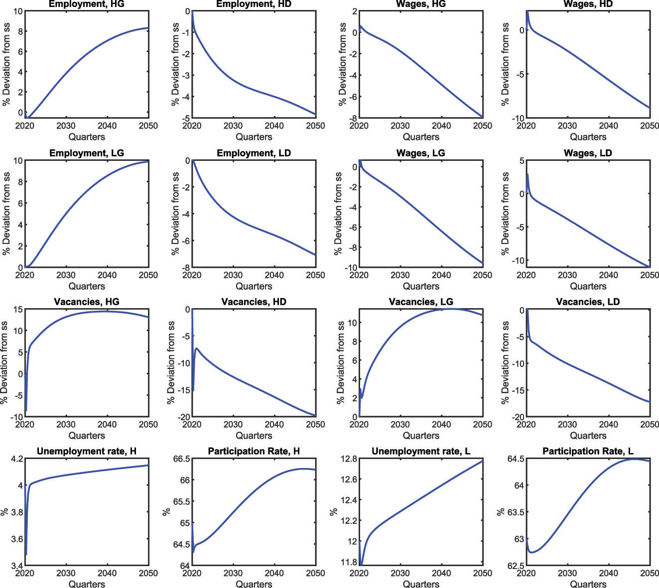
Transition to a net zero economy: labor market variables.
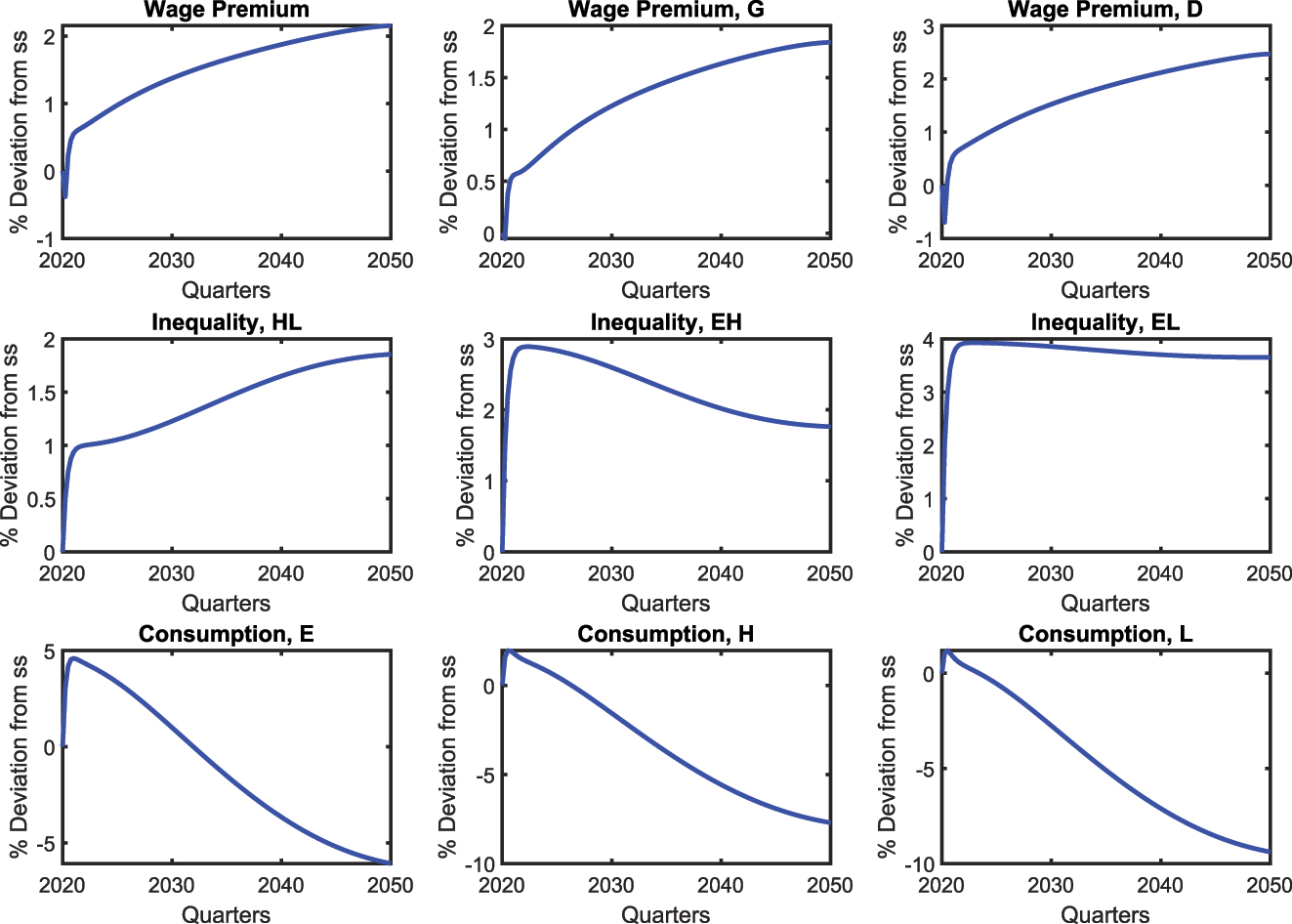
Transition to a net zero economy: inequality measures.
We first discuss the transition path of the baseline DSGE model with household heterogeneity.[10] The mechanism primarily impacts the dirty sector: as the tax on emissions gradually increases, firms in this sector respond by allocating more resources to abatement efforts. Both the carbon tax and the additional resources devoted to abatement reduce dirty firms’ marginal benefit of employing labor and accumulating capital by increasing their marginal costs. Consequently, dirty firms reduce their capital usage and post fewer vacancies leading to a decrease in dirty employment (−6 %) and production (−10 %). Given the presence of labor market frictions, the reallocation of employment from dirty to green firms is accompanied by a gradual but limited decrease in the aggregate employment rate. This mechanism negatively affects green output in the early stages of the transition. In the long run, green output and employment increase, reaching a peak of 8 % and 9 %, respectively. Consumption increases in the first quarters of the transition for all households. For workers, the increase is driven by a modest increase in wages in both sectors. Entrepreneurs increase their consumption due to a reduction in investment in the dirty sector and increased investment in the green sector.
Compared to the model without skills heterogeneity, the model presented in this paper shows a less significant negative impact on aggregate unemployment and output. In our model, employment in the green sector increases more substantially, while employment in the dirty sector experiences a sharper decline during the early stages of the transition. Nonetheless, by the end of the transition, employment in the dirty sector is reduced more significantly in the model without heterogeneity in the labor market. Additionally, while dirty production and employment decline more rapidly in the short term, their long-term decrease is less pronounced. In contrast, the model with worker heterogeneity predicts a greater increase in green production and employment, alongside a slower decline in wages.
These differences are closely related to the presence of heterogeneity among workers, particularly in terms of varying unemployment rates, asymmetry in the matching process, and differences in bargaining power.[11] SAM frictions imply that the transition to a new steady state may take time and can be associated with short-term costs in terms of employment, consumption, and production. Nonetheless, the presence of workers with diverse skills and bargaining powers facilitates a more flexible adjustment between sectors and labor market states, mitigating these costs. Additionally, the decline in consumption reduces the utility derived by workers from leisure, thereby explaining the observed increase in aggregate employment during the transition period.
As shown in Figure 2, our model captures the different structures of the labor market for high- and low-skilled workers. Although labor market frictions make the reallocation of employment from dirty to green firms more complex, the relatively large proportion of low-skilled workers available and their lower bargaining power compared to high-skilled workers facilitate green firms’ ability to increase the opening of vacancies for low-skilled workers from the early stages of the transition, in both sectors. After two quarters, green firms also begin to create new opportunities for high-skilled workers. Furthermore, vacancies in the dirty sector decline more rapidly for highly skilled workers than for low-skilled workers. These findings align with empirical literature, which finds that the skill requirements of green jobs are more similar to those of brown jobs than those of other sectors. Consequently, displaced workers in carbon-intensive industries can be successfully reemployed in emerging green jobs (Vona et al. 2023; Popp et al. 2022). These dynamics align with projections of the OECD (2023), which indicate that the initial phases of the transition to green jobs will predominantly involve a shift towards medium- and low-skilled occupations.
The combined increase in employment rates in the green sector captures differences in aggregate employment rise. At the end of the transition, the employment of skilled and unskilled workers increases by (8 %) and (10 %), respectively. Moreover, both dirty and green sector wages experience initial increments due to shifts in labor market equilibrium and reallocation dynamics. Wages in the dirty sector are chiefly influenced by household labor supply variables (
The wage premiums between high- and low-skilled workers experience a slight decline during the early stages of the transition, with this effect being more pronounced in the dirty sector. This is primarily due to the reallocation of low-skilled workers to the green sector. Nonetheless, in the long run, the transition toward a net-zero economy leads to an increase in wage premiums across all sectors and at the aggregate level. In terms of consumption, Figure 3 shows how the green transition increases the inequality between low-skilled workers and high-skilled workers and entrepreneurs. Moreover, disparities between entrepreneurs and high-skilled workers become more pronounced over time, further highlighting the widening inequality brought about by the transition.
5.2 Green Transition and Revenue Recycling Schemes
The baseline simulation assumes a transition toward a net zero economy without implementing carbon tax rebates. In this section, we examine three distinct carbon revenue recycling mechanisms:[12] (i) a uniform income tax cut, (ii) a progressive income tax cut, and (iii) unemployment benefits for both households. In the first and second mechanisms, carbon tax revenues are allocated to reduce labor income taxes. The first approach involves a uniform reduction in labor income taxes, applying the same rate of reduction across all worker groups. This is formalized as
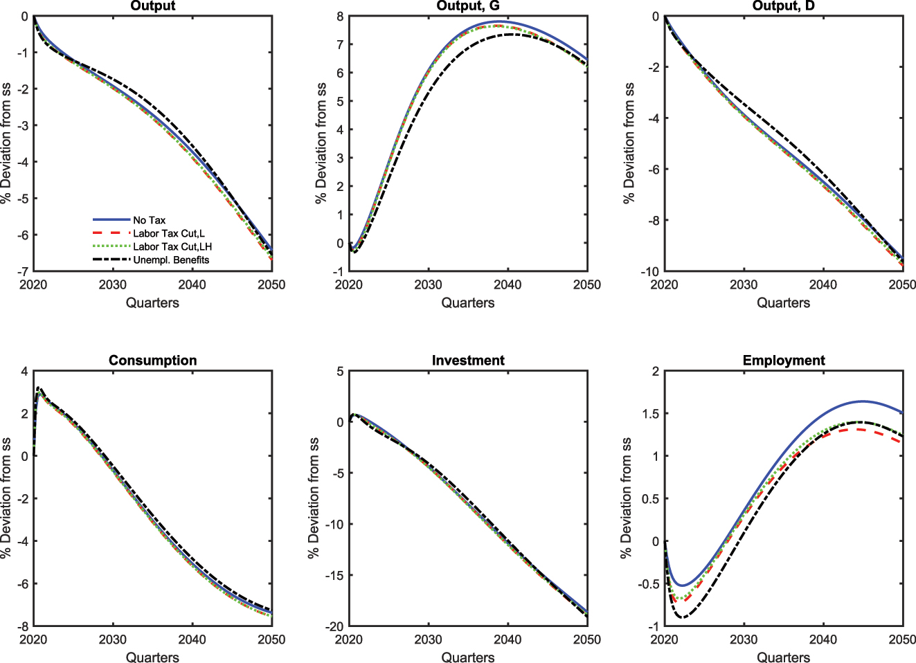
Figure 4 illustrates the labor market dynamics during the transition to a net-zero economy under various carbon revenue recycling schemes. The differing sensitivities of high- and low-skilled workers to these policies are evident in Figure 4: employment and wages for high-skilled workers exhibit smaller fluctuations compared to those of low-skilled workers across all policy scenarios. This disparity stems from the income effect, which has a more pronounced impact on low-skilled workers, which diminishes their propensity to supply labor.
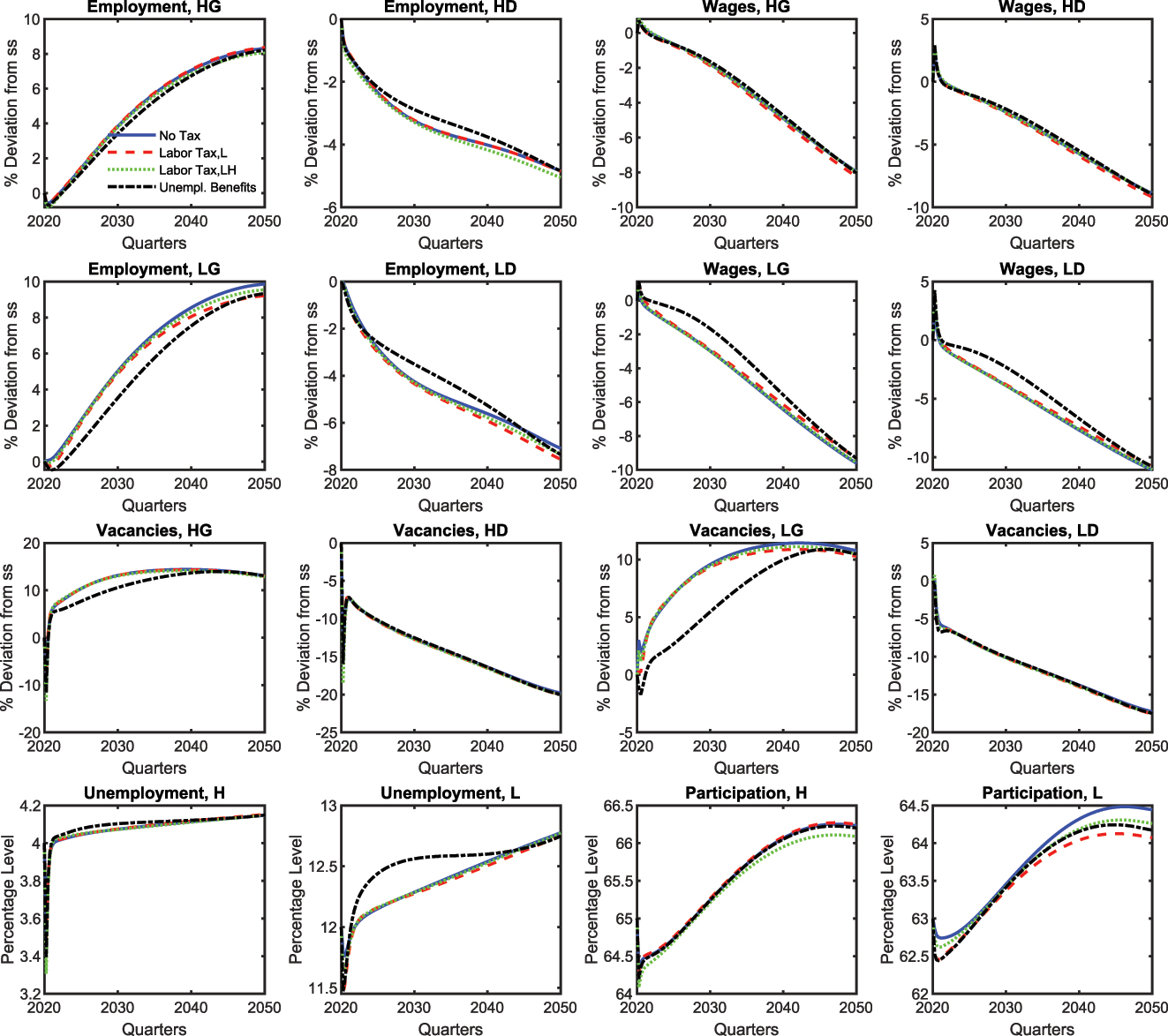
Transition to a net-zero economy and carbon recycling schemes: labor market variables. Note: The solid blue line (“No Tax”) represents the baseline simulation conducted without carbon revenue recycling policies. The red dashed line (“Labor Tax, L”) illustrates the effects of a progressive income tax reduction. The green dotted line (“Labor Tax, LH”) depicts a uniform income tax reduction that favors low-skilled workers. The black dashed-dotted line (“Unemp. Benefits”) indicates the provision of unemployment benefits to households.
Among the policies analyzed, unemployment benefits and the progressive labor income tax cut have the most significant short-term effects, particularly in reducing participation rates and vacancies in the green sector for low-skilled workers. The introduction of unemployment benefits leads to a decline in labor market participation during the early stages of the transition. This outcome is largely driven by the income effect, as financial support from unemployment benefits encourages individuals to substitute work with leisure. Similarly, the progressive labor income tax cut reduces incentives for low-skilled workers to participate in the labor market. This is due to the redistribution effect of such policies, which lowers the marginal utility of labor income relative to leisure, further reducing the drive to participate.
In the long term, unemployment benefits prove more effective than the progressive labor income tax cut in boosting labor market participation and employment among low-skilled workers. Employment in the green sector experiences faster growth under the unemployment benefits policy, particularly after the initial adjustment period. This dynamic is largely due to the role of unemployment benefits in facilitating smoother transitions for displaced workers from the dirty to the green sectors. By providing a safety net, unemployment benefits allow low-skilled workers to retrain or search for new opportunities in green sectors, which becomes particularly beneficial as green sector employment opportunities expand during the later stages of the transition.
The progressive labor income tax cut, on the other hand, introduces disincentives for low-skilled workers to participate in the labor market, particularly during the early stages of its implementation. Participation rates remain lower compared to unemployment benefits during the first phase of the transition. The reduced participation stems from the redistribution effect, which provides financial relief but lowers the marginal returns to labor for low-skilled workers. Consequently, while this policy drives positive outcomes, such as increased disposable income for low-skilled households, it falls short in addressing the structural challenges of reallocating labor to green sectors.
Nonetheless, the progressive labor income tax cut contributes, in the medium term, to higher employment in green sectors and a corresponding reduction in employment in dirty sector. This effect becomes prominent when revenues from the carbon tax (and consequently
In terms of job vacancies, these policies have a significant influence on openings for low-skilled workers in the green sector. Under unemployment benefits, the rate of vacancy creation in the green sector is notably slower compared to other policies. This slower growth in job openings reflects the immediate income support provided by unemployment benefits, which reduces the urgency for low-skilled workers to re-enter the labor market or transition to green sector jobs. Consequently, the slower vacancy growth moderates the supply-demand dynamics in the labor market, contributing to a more gradual decline in wages within the green sector.
A similar trend is observed in the dirty sector, where unemployment benefits lead to a smaller reduction in both production and employment levels for low-skilled and high-skilled workers. This occurs because unemployment benefits enable displaced workers from the dirty sector to temporarily remain out of the labor force rather than accepting lower wages in either green or dirty sector jobs. This dynamic eases immediate pressure on wages and production in the dirty sector, delaying the transition but also mitigating short-term economic disruptions.
Figure 5 illustrates the evolution of aggregate variables and sectoral output under various carbon revenue recycling strategies during the green transition. Sectoral dynamics play a crucial role in shaping the overall evolution of total employment, which experiences a sharper reduction at the beginning of the transition. This initial reduction is largely driven by policies that reduce incentives for labor market participation due to higher costs and the income effect. Over the course of the transition, as revenues increase, this gap is partially closed. However, a reduction in labor taxes for low-skilled workers results in a more pronounced reduction in total employment by 2050 compared to other policies. From a sectoral perspective, it is notable that unemployment benefits slow the expansion of the green sector while also decelerating the reduction in dirty sector production. Nevertheless, in terms of aggregate output, the labor tax cut for low-skilled workers entails a higher cost during the green transition.
Transition to a net zero economy and carbon recycling schemes: aggregate variables. Note: The solid blue line (“No Tax”) represents the baseline simulation conducted without carbon revenue recycling policies. The red dashed line (“Labor Tax, L”) illustrates the effects of a progressive income tax reduction. The green dotted line (“Labor Tax, LH”) depicts a uniform income tax reduction that favors low-skilled workers. The black dashed-dotted line (“Unemp. Benefits”) indicates the provision of unemployment benefits to households.
Figure 6 highlights the role of carbon revenue recycling schemes in reducing worker inequality throughout the green transition, while also showcasing their effects on aggregate variables and sectoral output under varying policy scenarios. The policies that strongly impact inequality during the green transition are labor tax cuts for low-skilled workers and unemployment benefits. The dynamics of the wage premium in both sectors are non-linear. Unemployment benefits help reduce wage inequality primarily in the medium term, while the progressive labor tax cut has an impact both in the early quarters of the transition and in the later stages. Additionally, the progressive labor tax cut allows for a permanent reduction in consumption-based inequality, providing a lasting improvement in equity throughout the transition.
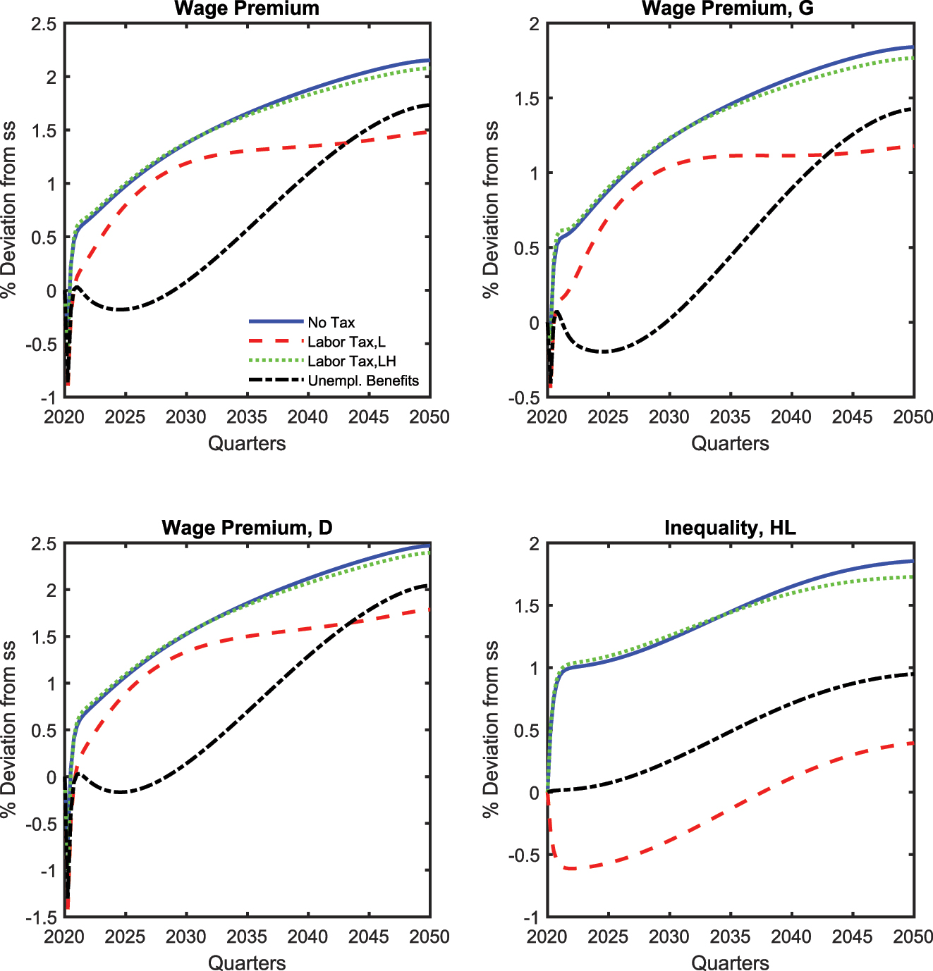
Transition to a net zero economy and carbon recycling schemes: inequality measures. Note: The solid blue line (“No Tax”) represents the baseline simulation conducted without carbon revenue recycling policies. The red dashed line (“Labor Tax, L”) illustrates the effects of a progressive income tax reduction. The green dotted line (“Labor Tax, LH”) depicts a uniform income tax reduction that favors low-skilled workers. The black dashed-dotted line (“Unemp. Benefits”) indicates the provision of unemployment benefits to households.
In summary, the figures indicate that both unemployment benefits and labor income tax cuts for low-skilled workers can significantly reduce the wage premium during the transition. In addition, labor income tax cuts for low-skilled workers also permanently reduce inequality in terms of consumption. However, both measures introduce distortions in the labor market by decreasing employment incentives for low-skilled workers. Aggregate output, consumption, and investment decrease in all scenarios. This decline is more pronounced when labor income tax cuts are implemented for low-skilled workers, indicating that the disincentive effects on labor participation outweigh any positive substitution effects. The choice of policy mix for recycling carbon tax revenues is crucial in shaping the dynamics of the green transition and its long-term distributional outcomes. To achieve a balance between equity and efficiency, these policies must be carefully designed and implemented.
5.3 Green Transition and Structural Change in the Green Sector
The results presented in the previous section are based on the assumption that the share of low-skilled workers in the green sector remains constant throughout the reference period. In this section, we examine the macroeconomic implications of a scenario in which the demand for low-skilled labor increases over time, consistent with projections from CEDEFOP (2021) and OECD (2023).[14]
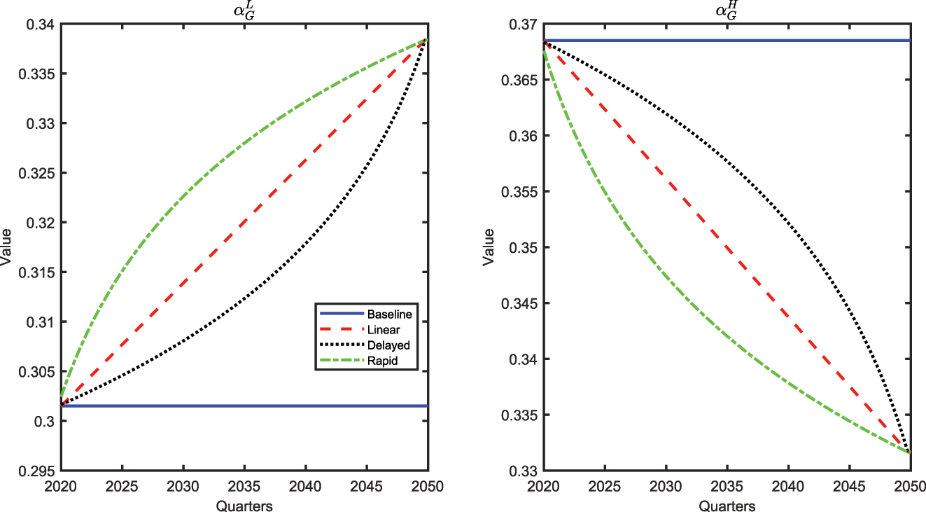
To address these questions, we assume a moderate increase of 10 % in the share of low-skilled workers
Figure 7 illustrates the labor market implications of the green transition under three scenarios involving an increase in the parameter
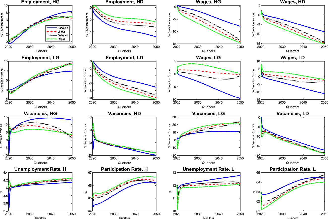
Transition to a net-zero economy under alternative adjustment paths for
In the dirty sector, the dynamics differ: vacancies for low-skilled workers decline more significantly, while in the initial quarters of the transition, more vacancies are opened for high-skilled workers, even in the dirty sector. These shifts in vacancy openings influence employment and wages across sectors and skill types. Employment of high-skilled workers in the green sector experiences greater growth during the early stages of the green transition and declines less significantly in the dirty sector. In contrast, low-skilled workers in the green sector exhibit an opposite trend, with slower growth in employment during the initial stages. In the dirty sector, employment for low-skilled workers decreases substantially.
The “rapid sectoral adjustment” scenario results in the most significant reduction in low-skilled employment within the dirty sector. While it promotes greater growth in green-sector employment, the employment rate by the end of the transition remains lower than in other scenarios, though still higher than the baseline case Participation rates decrease significantly and persistently for low-skilled workers. Only under the “delayed sectoral adjustment” scenario do low-skilled workers achieve a participation rate higher than the baseline case. The opposite occurs for highly skilled workers. For highly skilled workers, an increase in participation rates leads to a rise in unemployment, suggesting that higher participation does not necessarily translate into greater employment opportunities in the labor market. Conversely, for low-skilled workers, unemployment rates decrease during the early stages of the green transition, driven by a reduction in participation rates.
On the other hand, as the transition progresses, the unemployment rates remain close to the initial levels and lower than those observed in the baseline case. The greater availability of job openings for high-skilled workers, coupled with increased employment, leads to a reduction in wages for high-skilled workers in both sectors across the three scenarios considered, particularly under the “rapid sectoral adjustment” scenario. In contrast, the reduced presence of low-skilled workers in both sectors during the early stages of the transition allows wages for low-skilled workers to rise, remaining higher than in the baseline case throughout the transition. Among the scenarios considered, the “rapid sectoral adjustment” scenario provides the greatest wage benefits for low-skilled workers.
Figure 8 illustrates the macroeconomic dynamics of the green transition, showcasing the evolution of selected aggregate variables in response to a gradual increase in the share of low-skilled labor within the green sector. This structural adjustment plays a pivotal role in influencing labor allocation and reshaping the sectoral composition of the workforce, driving the dynamics of key aggregate variables throughout the transition. In the early stages, the shift in green production causes a slight decline in employment within the green sector. However, by approximately 2030, employment growth in the green sector accelerates, by exceeding the levels observed in the baseline model.
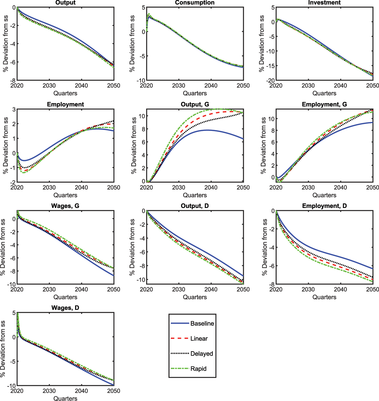
Transition to a net-zero economy under alternative adjustment paths for
In contrast, employment in the dirty sector decreases at a faster rate than in the baseline model. At the aggregate level, employment experiences a more pronounced reduction during the early stages of the transition. It is only in the final quarters of the transition that aggregate employment surpasses the levels observed in the baseline scenario. These labor market shifts lead to significant changes in productivity in both sectors. The green sector benefits from the structural shift, enabling a more efficient utilization of the workforce and resulting in enhanced production. Conversely, the dirty sector experiences a faster decline in output. In general, a smaller reduction in wages is observed in both sectors. These dynamics contribute to a more pronounced decrease in aggregate output. Nevertheless, the effects on aggregate investment and consumption remain negligible.
Figure 9 illustrates the implications of structural changes in the green sector for inequality throughout the green transition. The structural change in the workforce composition of the green sector allows low-skilled workers to benefit from wage improvements relative to high-skilled workers, thus permanently reducing the wage premium in both sectors. Moreover, this contributes to a reduction in consumption inequalities between workers. Specifically, a “rapid sectoral adjustment” increase in the share of low-skilled workers within the green sector leads to significant improvements in wage and consumption disparities, favoring low-skilled workers.
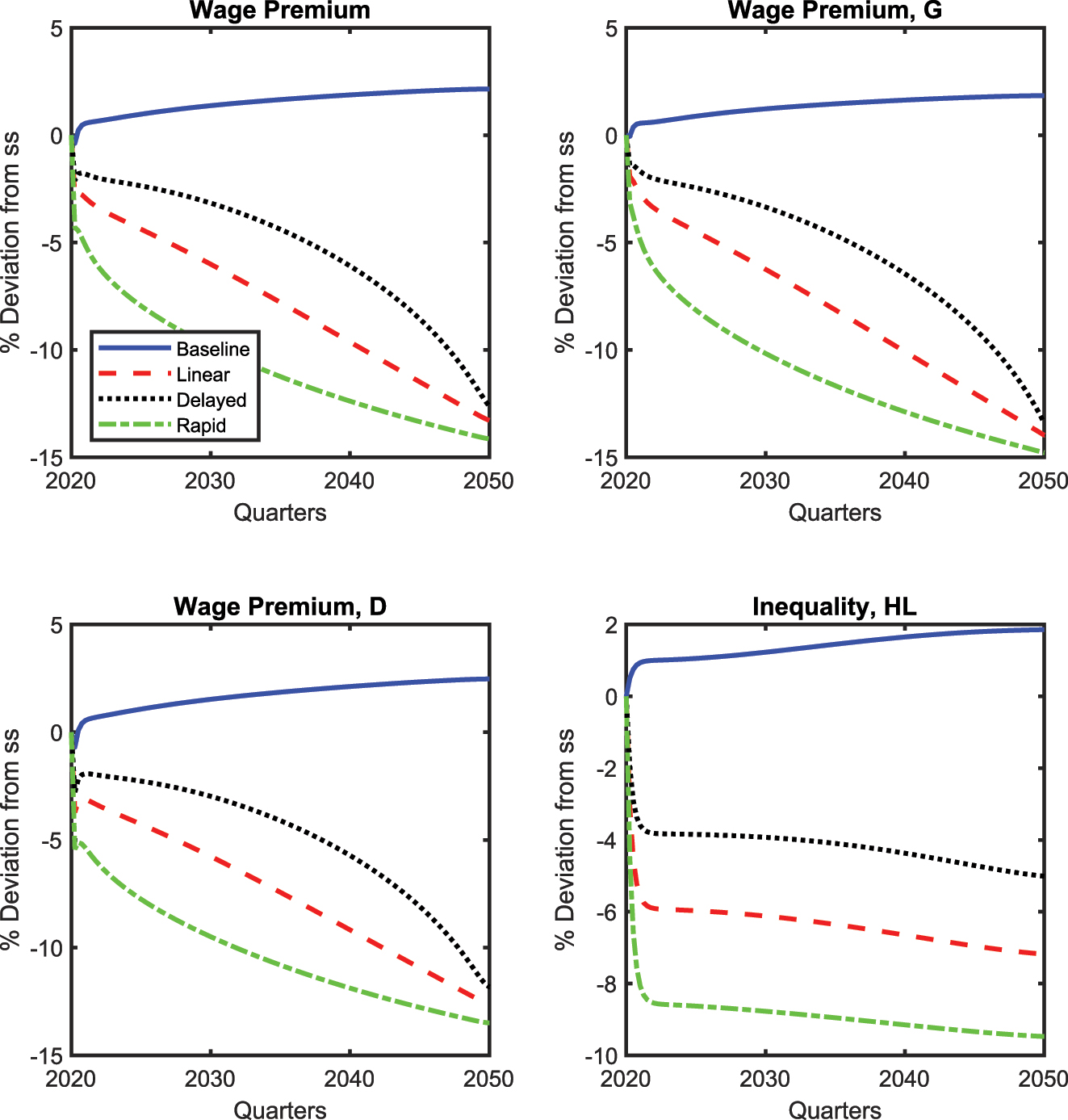
Transition to a net-zero economy under alternative adjustment paths for
In summary, the “rapid sectoral adjustment” scenario proves to be the most effective in reducing wage and consumption inequalities. It delivers early wage improvements for low-skilled workers, narrows the wage premium, and fosters more equitable outcomes. This scenario also results in the largest wage gains for low-skilled workers. In contrast, the “delayed sectoral adjustment” scenario, while boosting low-skilled employment rates by the end of the transition, postpones their integration into the green sector, thereby prolonging inequalities during the early stages of the transition. The gradual linear scenario offers greater stability throughout the transition but lacks the dynamic benefits and inequality reduction achieved under the “rapid sectoral adjustment” scenario.
6 Welfare Analysis
This section analyses the welfare implications of transitioning to a net-zero economy for both high-skilled and low-skilled workers. The welfare measure used is the unconditional expectation of the household’s lifetime utility function, defined as:
We perform a welfare analysis over various time horizons, examining the fiscal policy implications and their impacts on different worker groups. In addition, we assess the welfare costs associated with the transition to a net-zero economy and the role of labor market structure.[15]
Table 2 presents the welfare costs for high-skilled workers (ΔW H ), low-skilled workers (ΔW L ) and aggregate welfare (ΔW T ) across various carbon revenue recycling schemes and time horizons. It displays both the welfare changes relative to a steady state without carbon taxation and the percentage deviations from the baseline model for each group.
Welfare dynamics during the green transition under different carbon recycling schemes.
| Scenario | ΔW H | ΔW L | ΔW T |
|---|---|---|---|
| 2 years | |||
| Baseline | −4.872 | −6.528 | −5.413 |
| Progressive income tax cut | 1.383 | 2.000 | 1.628 |
| % Deviation from baseline | (+5.96 %) | (+8.01 %) | (+6.64 %) |
| Uniform income tax cut | 2.199 | 1.183 | 1.348 |
| % Deviation from baseline | (+6.74 %) | (+7.24 %) | (+6.38 %) |
| Unemployment benefits | 1.497 | 1.485 | 1.339 |
| % Deviation from baseline | (+6.07 %) | (+7.52 %) | (+6.36 %) |
| 10 years | |||
| Baseline | −6.791 | −8.657 | −7.266 |
| Progressive income tax cut | −1.603 | −1.208 | −1.197 |
| % Deviation from baseline | (+4.86 %) | (+6.86 %) | (+5.61 %) |
| Uniform income tax cut | −0.760 | −2.041 | −1.480 |
| % Deviation from baseline | (+5.65 %) | (+6.09 %) | (+5.36 %) |
| Unemployment benefits | −1.363 | −1.622 | −1.388 |
| % Deviation from baseline | (+5.08 %) | (+6.47 %) | (+5.43 %) |
| 30 years | |||
| Baseline | −8.839 | −10.922 | −9.246 |
| Progressive income tax cut | −8.652 | −9.103 | −8.067 |
| % Deviation from baseline | (+0.17 %) | (+1.64 %) | (+1.07 %) |
| Uniform income tax cut | −7.958 | −9.872 | −8.347 |
| % Deviation from baseline | (+0.81 %) | (+0.95 %) | (+0.82 %) |
| Unemployment benefits | −8.359 | −9.420 | −8.180 |
| % Deviation from baseline | (+0.44 %) | (+1.35 %) | (+0.96 %) |
-
Note: The table reports welfare changes (ΔW H ) for high-skilled workers, (ΔW L ) for low-skilled workers, and ΔW T as the weighted sum: (φ H ΔW H + φ L ΔW L ) for 2, 10, and 30 years. Values represent absolute welfare changes compared to the initial level for each group, while the % deviation from baseline indicates the percentage improvement relative to the baseline scenario with no fiscal intervention.
In the baseline scenario, which assumes no fiscal policy intervention, both high-skilled and low-skilled workers experience progressively increasing welfare losses over time. For high-skilled workers, the welfare decreases by −4.87 after two years, −6.79 after 10 years, and −8.84 after 30 years. Conversely, the impact on low-skilled workers is even more severe, with welfare losses amounting to −6.53, −8.66, and −10.92 over the same periods. These findings highlight the substantial costs associated with the transition, particularly in the absence of fiscal policies designed to mitigate its effects. These higher welfare losses of low-skilled workers point not only to a heterogeneous cost distribution but also, importantly, to structural difficulties of an equitable transition. Unless certain policy interventions-from income support and retraining programs to fiscal policies to redistribute costs-the current burden of transition falls increasingly on low-skilled workers, adding to ongoing inequalities within both the labor and wider economy.
The progressive income tax cut significantly mitigates short-term and long-term welfare losses for low-skilled workers, leading to an 8.01 % improvement in their welfare relative to the baseline after two years. Although the benefits persist over longer horizons, they diminish in magnitude, with deviations of 6.86 % after 10 years and 1.64 % after 30 years. High-skilled workers also experience welfare gains under this policy, albeit more modest ones. Their welfare increases by 1.38 after two years (5.96 % deviation from the scenario without carbon recycling schemes) but shows smaller long-term gains, with deviations of 4.86 % and 0.17 % after 10 and 30 years, respectively. These results suggest that progressive tax cuts prioritize redistribution toward the most vulnerable workers while still offering significant aggregate welfare improvements.
By contrast, the uniform income tax cut distributes benefits more evenly between skill groups but with less pronounced support for low-skilled workers. High-skilled workers see welfare improvements of 2.20 after 2 years (6.74 % deviation), followed by −0.76 after 10 years (5.65 % deviation) and −7.96 after 30 years (0.81 % deviation). Low-skilled workers also benefit from the uniform tax cut, but the improvements are more moderate compared to the progressive approach. The initial welfare improvements are notable (7.24 % for low-skilled workers after 2 years), yet over the long term, the policy does not provide the same level of targeted support. The diminishing effects suggest that, while the uniform tax cut reduces transition costs equitably, it is less effective in addressing structural disadvantages faced by low-skilled workers, as indicated by their relatively higher long-term welfare losses.
Unemployment benefits emerge as an effective short-term buffer for low skilled workers, with welfare increases of 7.52 % after two years, slightly surpassing the uniform tax cut’s impact. These short-run gains can be attributed to the fact that unemployment benefits provide financial support for workers during the immediate economic disruptions of the transition, such as job loss and income loss. However, this measure consistently under-performs compared to the other policy options for high-skilled workers.
In terms of aggregate welfare, the most effective strategy for mitigating the economic costs of the green transition is the progressive income tax cut, which provides the highest overall welfare gains. It offers targeted support to low-skilled workers, who are most vulnerable to labor market disruptions, while also delivering measurable benefits to high-skilled workers. Despite this, a more balanced approach emerges when considering medium- and long-term dynamics. Shifting revenue recycling toward unemployment subsidies proves more effective than a uniform income tax cut, as it better addresses labor market dislocations and fosters greater structural adaptability, ensuring higher resilience to long-term transition costs.
These findings underscore the importance of designing carbon tax revenue recycling strategies that effectively balance short-term mitigation of distributional impacts with long-term economic adaptability. Such a design is essential to ensure that both equity and efficiency considerations are adequately addressed in the transition toward net-zero emissions.
7 Sensitivity Analysis
This section provides a sensitivity analysis on critical parameters
7.1 The Role of Asymmetry in the Labor Market
This section explores alternative baseline calibrations of the benchmark model, assuming:(1) symmetry in the matching elasticity
7.2 Welfare and Labor Market Asymmetry
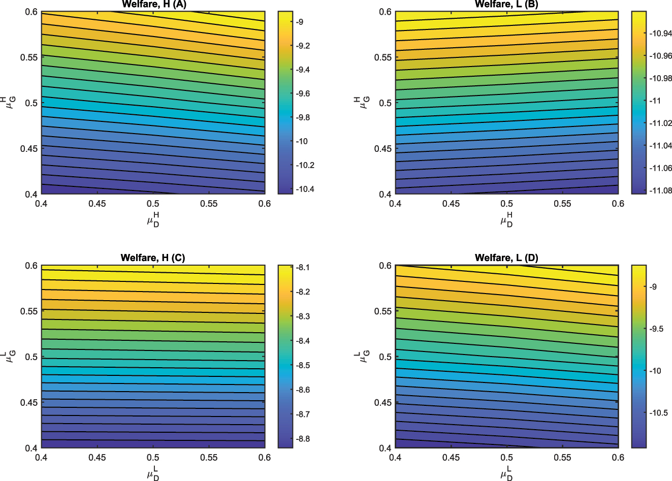
In the baseline calibration, we account for the asymmetry between workers while maintaining the symmetry between sectors regarding the labour market structure. In this section, we evaluate the critical characteristics of the sectoral labor market that influence welfare costs during the transition. To achieve this, we examine the welfare of high- and low-skilled households by conducting a sensitivity analysis of key structural parameters. Figure B.3 illustrates the sensitivity of welfare to the elasticity of unemployment in the matching function
7.3 Alternative Calibration: Services and Manufacturing Sectors
In the baseline calibration, we differentiate between green and dirty goods based on the energy sources used in production, following Carattini et al. (2021) and Giovanardi et al. (2021). However, according to Ferrari and Nispi Landi (2023), in this section, we reinterpret the green sector as the service sector and the brown sector as the manufacturing sector. We set the share of green production to 0.65 and apply an elasticity of substitution of 0.5 for the euro area, as in Ferrari and Nispi Landi (2023). Figures B.8–B.10 illustrate the transition for aggregate variables, the labor market, and inequality under this alternative calibration. Although this calibration yields results that are consistent with the baseline, it reveals notable differences in the dynamics of the transition. The limited substitutability between green and non-green products, along with the share of polluting sectors, plays a crucial role in shaping the green transition. Under this alternative calibration, the decline in aggregate output and dirty sector variables is less pronounced. In the initial phase of the transition, job vacancies in the green sector open at a faster rate, leading to a gradual rise in unemployment within these sectors. At the same time, participation rates increase, which subsequently increases the overall unemployment rate. Finally, although inequality trends remain consistent with the baseline results, their impact is less pronounced in this context.
8 Conclusions
This paper examines the long-term quantitative impact of a carbon tax on labor market dynamics and distributional implications within a model that incorporates worker heterogeneity and unemployment. We examine the transition toward a net-zero economy from the first quarter of 2019–2050, with a gradual increase in the carbon tax.
The relevant conclusions of this paper for policy-makers are that market forces alone will not ensure a just transition to net zero emissions. Without policy intervention, a green transition could prove socially regressive and disproportionately burden low-skilled workers. Therefore, it requires a proactive policy approach to ensure that environmental sustainability is achieved in a socially inclusive manner. In this regard, our results show that no single measure will be sufficient to address the economic and social challenges posed by the green transition. A progressive labor income tax cut reduces the transition costs for low-skilled workers, who are the most affected by this shift. Nevertheless, at the same time, this policy creates a significant gap in the benefits received by the two types of workers. Moreover, these measures have different impacts on the skill wage premium and consumption inequality at various stages of the transition. Redistributive policies must, therefore, be combined to ensure that the transition is both economically viable and at the same time environmentally effective and socially fair. Without such measures, there is a continued risk that the benefits of a net-zero economy will not be distributed evenly and may actually widen existing inequalities rather than creating an inclusive, sustainable future. Other measures for addressing inequalities involve reducing asymmetry between workers and sectors in the labor market. In this sense, governments could actively support structural shifts within the green economy by providing targeted training, incentivizing employers to hire low-skilled workers in green-sector firms, and ensuring that fiscal policies are adjusted to promote workforce diversification.
This paper represent is an initial exploration of the interplay between skill differences, inequality, and the effectiveness of carbon revenue recycling policies during the green transition, using an E-DSGE framework. A key contribution of this study is its emphasis on the complex composition of the workforce, which could be further expanded to include a broader range of worker categories and sectors with distinct labor demands. Moreover, this study has focused on redistributive fiscal policies while excluding those aimed at supply-side promotion. Exploring these dimensions represents a valuable opportunity for future research.
Appendix A: Additional Figures
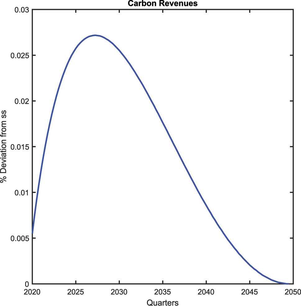
Transition to a net zero economy: carbon tax revenues.
Transition dynamic for
Appendix B: Sensitivity Analysis
B.1 The Role of Asymmetry in the Labor Market
Table B.1 presents the impact of the green transition on various inequality measures, comparing both the initial steady-state levels at time t = 1 and the relative changes observed in the long-run equilibrium at t = 120.
Sensitivity analysis on
| Scenario |
|
|
|
Ineq. H,L | Ineq. E,H | Ineq. E,L |
|---|---|---|---|---|---|---|
| Baseline model | ||||||
| Asymmetric (t = 1) | 2.51 | 2.51 | 2.51 | 2.83 | 4.13 | 11.69 |
| Asymmetric (t = 120) | 2.15 | 1.84 | 2.47 | 1.85 | 1.76 | 3.65 |
| Symmetric
|
−1.68 | −1.68 | −1.68 | −1.68 | 2.07 | 0.36 |
| Symmetric
|
−1.98 | −2.02 | −1.93 | −2.03 | 2.14 | 0.07 |
| Symmetric
|
−1.22 | −1.22 | −1.22 | −1.22 | 0.12 | −1.10 |
| Symmetric
|
−3.13 | −3.41 | −2.85 | −2.54 | 0.79 | −1.77 |
| Symmetric
|
−1.78 | −1.78 | −1.78 | −1.78 | 1.29 | −0.52 |
| Symmetric
|
−1.92 | −1.93 | −1.92 | −1.85 | 1.32 | −0.56 |
| Symmetric (t = 1) | −4.64 | −4.64 | −4.64 | −4.64 | 3.88 | −0.94 |
| Symmetric (t = 120) | −6.87 | −7.19 | −6.55 | −6.29 | 4.62 | −1.96 |
B.2 Welfare and Elasticity of Matching
Figure B.3 shows the welfare sensitivity to the elasticity of unemployment in the matching function
Sensitivity analysis of matching efficiency in the green and dirty sectors.
Panel (A) shows the welfare sensitivity for high-skilled households to the elasticity of unemployment in the matching function for high-skilled workers in the green sector relative to changes in the dirty sector. When
B.3 Welfare and Separation Rates
Figure B.4 graphically reports welfare in terms of contour plots. Panel (A) investigates the sensitivity of our results to the separation rate for high-skilled workers in the green and dirty sectors, varying both within the range [0.04, 0.06]. Increases in the separation rate in both sectors decrease welfare for high-skilled workers, but a higher separation rate in the green sector has a more pronounced negative impact on welfare. In contrast, panel (B) illustrates how increased separation rates in the dirty sector mitigate the welfare cost of the transition for low-skilled workers, whereas higher separation rates in the green sector reduce welfare. The limited range of welfare changes indicates a slight spillover effect between the two markets. Panel (C) demonstrates the sensitivity of high-skilled welfare to low-skilled separation rates in both sectors within the range [0.04, 0.06]. An increase in the green sector’s separation rate for low-skilled workers negatively impacts high-skilled welfare due to a spillover effect. The opposite effect is observed when the separation rate increases in the dirty sector. High-skilled workers exhibit greater sensitivity to changes in the low-skilled market compared to low-skilled workers. Panel (D) reveals that increased separation rates lead to decreased welfare for low-skilled families, with a more pronounced effect compared to high-skilled families. The above analysis shows that increases in separation rates decrease welfare for both high-skilled and low-skilled workers, with a more pronounced negative impact in the green sector for high-skilled workers. Low-skilled workers benefit more from increased separation rates in the dirty sector, while high-skilled workers are more sensitive to changes in the low-skilled market. In summary, the changes in the separation rate exhibit spillover effects between the green and dirty sectors.
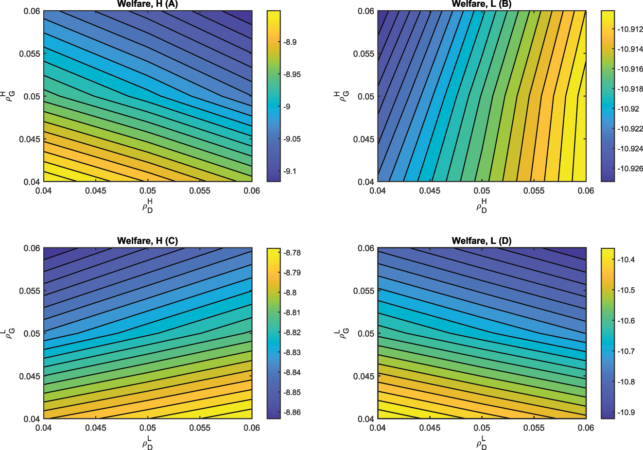
Sensitivity analysis on survival rate in the green and dirty sectors.
Figures B.5–B.7, below confirm that our main findings in the baseline model remain unchanged under alternative baseline calibrations for macroeconomic variables. In particular, we consider calibrations where: 1) symmetry in the matching elasticity
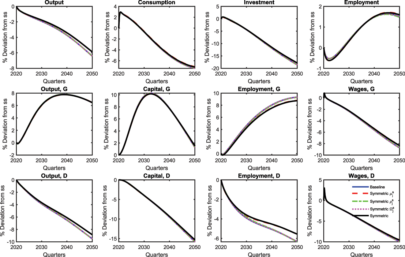
Robustness check on asymmetry in the labor market: aggregate variables.
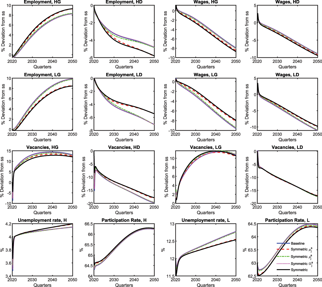
Robustness check on asymmetry in the labor market: labor market variables.
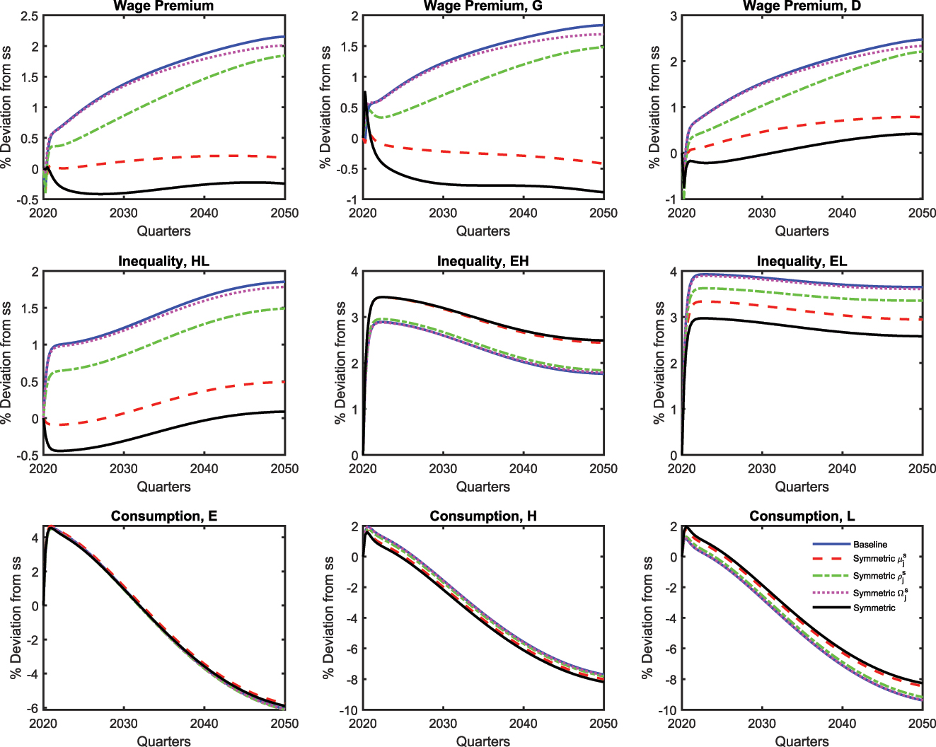
Robustness check on asymmetry in the labor market: inequality measures.
Figures B.8–B.10 illustrate the transition towards a net-zero economy, considering the green sectors as the service sector and the dirty sectors as the manufacturing sector (γ = 0.65, ξ = 0.5).
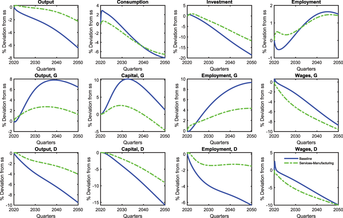
Alternative calibration – services and manufacturing: aggregate variables.
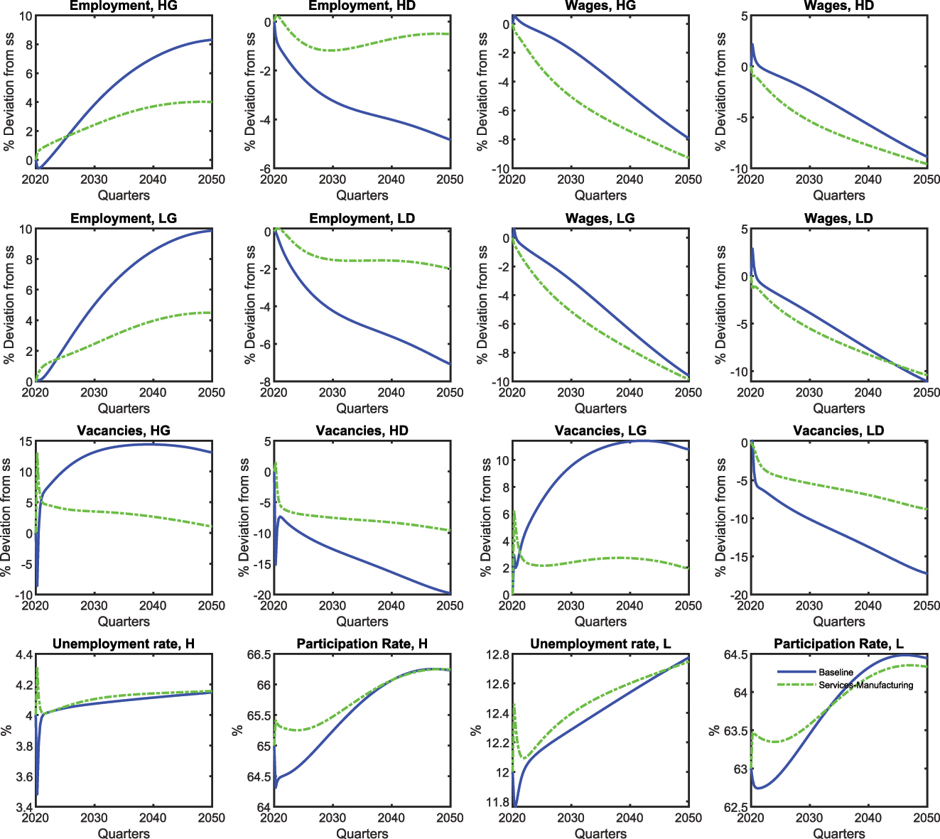
Alternative calibration – services and manufacturing: labor market variables.
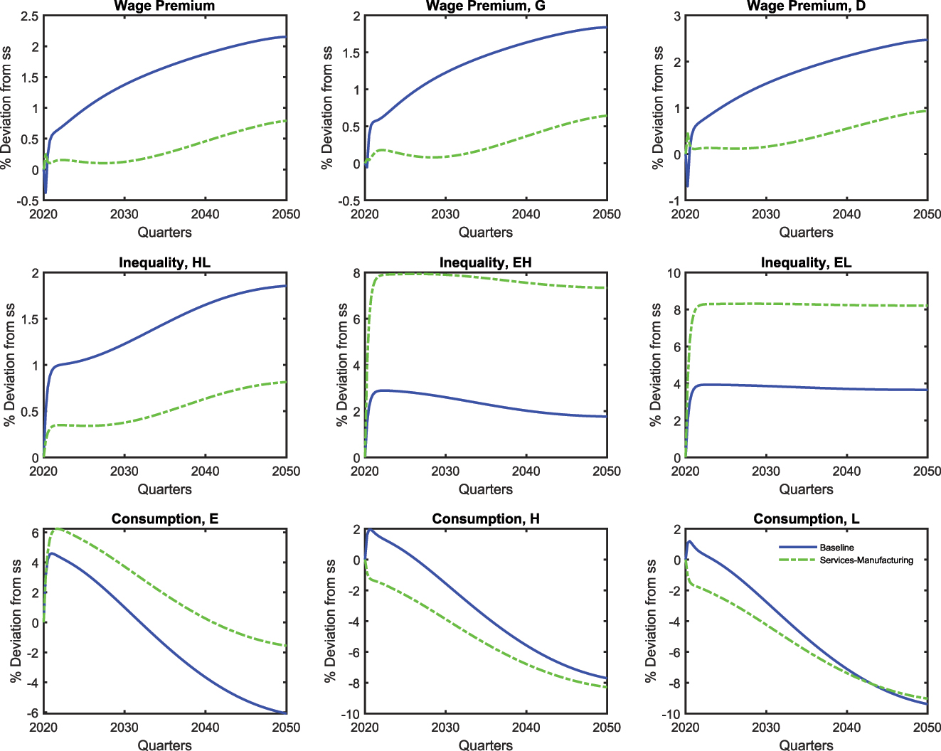
Alternative calibration – services and manufacturing: inequality measures.
References
Abbritti, M., and Consolo, A. 2022. Labour Market Skills, Endogenous Productivity and Business Cycles (ECB Working Paper No. 2651). Frankfurt am Main: European Central Bank.10.2139/ssrn.4046331Search in Google Scholar
Adjemian, S., H. Bastani, M. Juillard, F. Karame, F. Mihoubi, G. Perendia, J. Pfeifer, M. Ratto, and S. Villemot. 2011. Dynare: Reference manual (Version 4). CEPREMAP.Search in Google Scholar
Annicchiarico, B., and F. Di Dio. 2015. “Environmental Policy and Macroeconomic Dynamics in a New Keynesian Model.” Journal of Environmental Economics and Management 69: 1–21. https://doi.org/10.1016/j.jeem.2014.10.002.Search in Google Scholar
Aubert, D., and M. Chiroleu-Assouline. 2019. “Environmental Tax Reform and Income Distribution with Imperfect Heterogeneous Labour Markets.” European Economic Review 116: 60–82. https://doi.org/10.1016/j.euroecorev.2019.03.006.Search in Google Scholar
Benmir, G., and J. Roman. 2020. Policy Interactions and the Transition to Clean Technology. Grantham Research Institute on Climate Change and the Environment.Search in Google Scholar
Bowen, A., K. Kuralbayeva, and E. L. Tipoe. 2018. “Characterising Green Employment: The Impacts of ‘Greening’ on Workforce Composition.” Energy Economics 72: 263–75. https://doi.org/10.1016/j.eneco.2018.03.015.Search in Google Scholar
Carattini, S., Heutel, G., and Melkadze, G. 2021. “Climate Policy, Financial frictions, and Transition risk.” NBER Working Paper No. 28525. https://doi.org/10.3386/w28525.Search in Google Scholar
Castellanos, K. A., and G. Heutel. 2019. Unemployment, Labor Mobility, and Climate Policy (No. w25797). National Bureau of Economic Research. http://www.nber.org/papers/w25797.10.3386/w25797Search in Google Scholar
Chen, Z., G. Marin, D. Popp, and F. Vona. 2020. “Green Stimulus in a Post-Pandemic Recovery: The Role of Skills for a Resilient Recovery.” Environmental and Resource Economics 76: 901–11. https://doi.org/10.1007/s10640-020-00464-7.Search in Google Scholar
Coenen, G., P. Karadi, S. Schmidt, and A. Warne. 2018. “The New Area-Wide Model II: An Extended Version of the Ecb’s Micro-Founded Model for Forecasting and Policy Analysis with a Financial Sector.” ECB Working Paper No. 2200.10.2139/ssrn.3287647Search in Google Scholar
Consoli, D., G. Marin, A. Marzucchi, and F. Vona. 2016. “Do Green Jobs Differ from Non-Green Jobs in Terms of Skills and Human Capital?” Research Policy 45 (5): 1046–60. https://doi.org/10.1016/j.respol.2016.02.007.Search in Google Scholar
Diluiso, F., B. Annicchiarico, M. Kalkuhl, and J. C. Minx. 2021. “Climate Actions and Macro-Financial Stability: The Role of Central Banks.” Journal of Environmental Economics and Management 110: 102548. https://doi.org/10.1016/j.jeem.2021.102548.Search in Google Scholar
Dolado, J. J., G. Motyovszki, and E. Pappa. 2021. “Monetary Policy and Inequality Under Labor Market Frictions and Capital-Skill Complementarity.” American Economic Journal: Macroeconomics 13 (2): 292–332. https://doi.org/10.1257/mac.20180242.Search in Google Scholar
Eeckhout, J., and P. Kircher. 2018. “Assortative Matching with Large Firms.” Econometrica 86 (1): 85–132, https://doi.org/10.3982/ECTA14450.Search in Google Scholar
Elliott, R. J., and J. K. Lindley. 2017. “Environmental Jobs and Growth in the United States.” Ecological Economics 132: 232–44. https://doi.org/10.1016/j.ecolecon.2016.08.001.Search in Google Scholar
European Commission. 2019. The European Green Deal (COM(2019) 640 final). Brussels: European Commission.Search in Google Scholar
Ferrari, A., and V. Nispi Landi. 2023. “Toward a Green Economy: The Role of Central Bank’s Asset Purchases.” International Journal of Central Banking 19 (5): 287–340.10.2139/ssrn.4357535Search in Google Scholar
Fischer, C., and M. Springborn. 2011. “Emissions Targets and the Real Business Cycle: Intensity Targets Versus Caps or Taxes.” Journal of Environmental Economics and Management 62 (3): 352–66. https://doi.org/10.1016/j.jeem.2011.04.005.Search in Google Scholar
Gagliardi, L., G. Marin, and C. Miriello. 2016. “The Greener the Better? Job Creation Effects of Environmentally-Friendly Technological Change.” Industrial and Corporate Change 25 (5): 779–807. https://doi.org/10.1093/icc/dtv054.Search in Google Scholar
Gathmann, C., and U. Schönberg. 2010. “How General is Human Capital? A Task-Based Approach.” Journal of Labor Economics 28 (1): 1–49. https://doi.org/10.1086/649786.Search in Google Scholar
Gibson, M., and G. Heutel. 2023. “The Business Cycle and the Environment: The Role of Environmental Policy.” Review of Environmental Economics and Policy 17 (1): 92–109. https://doi.org/10.1093/reep/rez022.Search in Google Scholar
Giovanardi, F., M. Kaldorf, L. Radke, and F. Wicknig. 2021. “The Preferential Treatment of Green Bonds.” Mimeo, https://ssrn.com/abstract=3841616.10.2139/ssrn.3841616Search in Google Scholar
Greenstone, M. 2002. “The Impacts of Environmental Regulations on Industrial Activity: Evidence from the 1970 and 1977 Clean Air Act Amendments and the Census of Manufactures.” Journal of Political Economy 110 (6): 1175–219. https://doi.org/10.1086/342808.Search in Google Scholar
Hafstead, M. A. C., and R. C. WilliamsIII. 2018. “Unemployment and Environmental Regulation in General Equilibrium.” Journal of Public Economics 160: 50–65. https://doi.org/10.1016/j.jpubeco.2018.01.013.Search in Google Scholar
Hagedorn, M., I. Manovskii, and K. Mitman. 2016. “The Impact of Unemployment Benefit Extensions on Employment: The 2014 Employment Miracle?” The American Economic Review 106 (5): 366–70. https://doi.org/10.3386/w20884.Search in Google Scholar
Heutel, G. 2012. “How Should Environmental Policy Respond to Business Cycles? Optimal Policy Under Persistent Productivity Shocks.” Review of Economic Dynamics 15 (2): 244–64. https://doi.org/10.1016/j.red.2011.05.002.Search in Google Scholar
Horbach, J., and K. Rennings. 2013. “Environmental Innovation and Employment Dynamics in Different Technology Fields – An Analysis Based on the German Community Innovation Survey 2009.” Journal of Cleaner Production 57: 158–65. https://doi.org/10.1016/j.jclepro.2013.05.034.Search in Google Scholar
Jackman, M., and W. Moore. 2021. “Does it Pay to be Green? An Exploratory Analysis of Wage Differentials Between Green and Non-Green Industries.” Journal of Economics and Development 23 (3): 284–98. https://doi.org/10.1108/JED-08-2020-0099.Search in Google Scholar
Kahn, M. E., and E. T. Mansur. 2013. “Do Local Energy Prices and Regulation Affect the Geographic Concentration of Employment?” Journal of Public Economics 101: 105–14. https://doi.org/10.1016/j.jpubeco.2013.03.002.Search in Google Scholar
Kudlyak, M., and E. Wolcott. 2018. “Skill Mismatch Unemployment.” In Meeting Papers from Society for Economic Dynamics (No. 1408).Search in Google Scholar
Marin, G., and F. Vona. 2019. “Climate Policies and Skill-Biased Employment Dynamics: Evidence from EU Countries.” Journal of Environmental Economics and Management 98: 102253. https://doi.org/10.1016/j.jeem.2019.102253.Search in Google Scholar
Monacelli, T., R. Perotti, and A. Trigari. 2010. “Unemployment Fiscal Multipliers.” Journal of Monetary Economics 57 (5): 531–53.10.1016/j.jmoneco.2010.05.009Search in Google Scholar
Mortensen, D. T., and C. A. Pissarides. 1994. “Job Creation and Job Destruction in the Theory of Unemployment.” The Review of Economic Studies 61 (3): 397–415. https://doi.org/10.2307/2297896.Search in Google Scholar
Nordhaus, W. D. 2008. A Question of Balance: Weighing the Options on Global Warming Policies. New Haven, CT: Yale University Press.10.2307/j.ctt1npzkhSearch in Google Scholar
OECD. 2023. Job Creation and Local Economic Development 2023: Bridging the Great Green Divide. Paris: OECD Publishing.Search in Google Scholar
Oikonomou, M. 2023. Migration, Search and Skill Heterogeneity. International Monetary Fund.10.2139/ssrn.4378197Search in Google Scholar
Pissarides, C. A., and B. Petrongolo. 2001. “Looking into the Black Box: A Survey of the Matching Function.” Journal of Economic Literature 39 (2): 390–431, https://doi.org/10.1257/jel.39.2.390.Search in Google Scholar
Popp, D., F. Vona, G. Marin, and Z. Chen. 2020. The Employment Impact of Green Fiscal Push: Evidence from the American Recovery Act (No. w27321). National Bureau of Economic Research.10.3386/w27321Search in Google Scholar
Popp, D., F. Vona, G. Marin, and Z. Chen. 2022. “Green Transition and Workforce Skills: A Task-Based Perspective.” Journal of Environmental Economics and Management 110: 102545. https://doi.org/10.1016/j.jeem.2021.102545.Search in Google Scholar
Ranieri, A. 2013. “Skills for a Low-Carbon Europe: The Role of VET in a Sustainable Energy Scenario.” Synthesis Report. Research Paper No 34. Cedefop-European Centre for the Development of Vocational Training.Search in Google Scholar
Saussay, A., M. Sato, F. Vona, and L. O’Kane. 2022. “Who’s Fit for the Low-Carbon Transition? Emerging Skills and Wage Gaps in Job Ad Data.” In Nota di Lavoro 31.2022, Milano, Italy: Fondazione Eni Enrico Mattei.10.21203/rs.3.rs-1649850/v1Search in Google Scholar
Shapiro, A. F., and G. E. Metcalf. 2023. “The Macroeconomic Effects of a Carbon Tax to Meet the US Paris Agreement Target: The Role of Firm Creation and Technology Adoption.” Journal of Public Economics 218: 104800. https://doi.org/10.1016/j.jpubeco.2022.104800.Search in Google Scholar
Shimer, R. 2005. “The Cyclical Behavior of Equilibrium Unemployment and Vacancies.” The American Economic Review 95 (1): 25–49. https://doi.org/10.1257/0002828053828572.Search in Google Scholar
Sun, T., X. Bian, J. Liu, R. Wang, and S. Sriboonchitta. 2023. “The Economic and Social Effects of Skill Mismatch in China: A DSGE Model with Skill and Firm Heterogeneity.” Economic Modelling 125: 106345. https://doi.org/10.1016/j.econmod.2023.106345.Search in Google Scholar
The Green Employment and Skills Transformation: Insights from a European Green Deal Skills Forecast Scenario (Publication No. 4206). 2021. Luxembourg: Publications Office.Search in Google Scholar
Vandeplas, A., I. Vanyolos, M. Vigani, and L. Vogel. 2022. The Possible Implications of the Green Transition for the EU Labour Market. Publications Office of the European Union. https://ec.europa.eu/info/publications/economic-and-financial-affairs-publications_en.Search in Google Scholar
Vona, F. 2023. “Managing the Distributional Effects of Climate Policies: A Narrow Path to a Just Transition.” Ecological Economics 205: 107689. https://doi.org/10.1016/j.ecolecon.2022.107689.Search in Google Scholar
Vona, F., G. Marin, D. Consoli, and D. Popp. 2015. Green Skills (No. w21116). National Bureau of Economic Research.10.3386/w21116Search in Google Scholar
Vona, F., G. Marin, D. Consoli, and D. Popp. 2018. “Environmental Regulation and Green Skills: An Empirical Exploration.” Journal of the Association of Environmental and Resource Economists 5 (4): 713–53. https://doi.org/10.1086/698859.Search in Google Scholar
Walker, W. R. 2011. “Environmental Regulation and Labor Reallocation: Evidence from the Clean Air Act.” The American Economic Review 101 (3): 442–7. https://doi.org/10.1257/aer.101.3.442.Search in Google Scholar
© 2025 the author(s), published by De Gruyter, Berlin/Boston
This work is licensed under the Creative Commons Attribution 4.0 International License.
Articles in the same Issue
- Frontmatter
- Advances
- Real Wage Cyclicality and Monetary Policy
- Green Transition, Skills Heterogeneity, and Inequality
- Workforce Aging, Growth and Productivity
- Monetary Policy Shocks: Data or Methods?
- Contributions
- Monetary Policy and Labor Market Friction in a HANK Model
- Capital Market Liberalization and Bank Credit Decisions: A Quasi-Natural Experiment Based on the “Mainland-Hong Kong Stock Connect”
- Automation, Skill Premium, and Labor Share
- Business Cycles, Monetary Policy Stance, and Monetary Policy Transmission in Korea
- Forecasting Revisions to U.S. Jobs Report Data
- Loan Loss Provision, Unsecured-Collateralized Loan Choice and Macro-Stability in China
- Price Stickiness, Input–Output Linkages, and Monetary Policy Transmission in Korea
- Oil Price-Driven Inflation and the Channels of Pass-Through
- Firm Dynamics, Informality, and Monetary Policy