
Monetary Policy Shocks: Data or Methods?
-
Connor M. Brennan

 ,
Christian Matthes
,
Christian Matthes

Abstract
Different series of high-frequency monetary shocks can have a correlation coefficient as low as 0.3 and the same sign in only one half of observations. Both data and methods drive these differences, which are starkest when the federal funds rate is at its effective lower bound. After documenting differences in monetary shock series, we explore their consequences for inference in several specifications. We find that empirical estimates of monetary policy transmission have few qualitative differences. We caution that inference may not be entirely robust to all shock constructions because qualitative differences can emerge when data and methods are interchanged.
1 Introduction
Because monetary policy simultaneously affects and responds to economic conditions, identifying its exogenous variation is an ongoing challenge. Any instrument that estimates monetary shocks must be orthogonal to economic conditions and control for all available information to isolate unanticipated decisions from anticipated. Since at least Kuttner (2001), high-frequency environments have proven useful to fine-tune information sets to extract market surprises. Asset prices observed minutes before a monetary policy decision presumably contain all available information and hence control for any anticipated decision. Asset prices observed minutes after a monetary policy decision reflect the market reaction to the decision. Because only monetary news is released in the narrow time window surrounding a decision, researchers can presumably isolate monetary surprises from non-monetary news.
Given that various high-frequency monetary shock series are constructed from highly correlated changes in asset prices in similar narrow time windows around the same monetary policy announcements, one could expect the series to have similar magnitudes and signs even if underlying data or statistical methods differ. We find that differences emerge in practice, especially when the federal funds rate is at its effective lower bound (ELB). We ask if data or methods drive these differences in high-frequency monetary shock series for the United States. For researchers studying the transmission of monetary policy to either financial markets or the macroeconomy, differences in monetary shock series could be particularly troubling if they lead to differences in estimates of the effect of monetary policy. In practice, we find that differences in monetary shock series affect the magnitudes of point estimates but only affect the sign in certain specifications. This finding is only robust to commonly used monetary policy shock series, as constructions that interchange data and methods – i.e., take the data from one series and use it in the method of another – have different signs of their point estimates.
The first contribution of this paper is to construct and compare commonly used monetary shock series from high-frequency trades so that readers without access to the underlying intraday tick-by-tick data can better understand the differences. Although high-frequency constructs are widely used, limited data availability often precludes construction from scratch [see Nakamura and Steinsson (2018), Acosta (2023), Boehm and Kroner (2025) and Nunes et al. (2023) for notable exceptions]. Among all of the numerous high-frequency series, we focus on seven: four that are commonly used – Kuttner (2001), Gertler and Karadi (2015), Nakamura and Steinsson (2018), and Bu et al. (2021) – and three that interchange data and methods. Like Swanson (2023) and Bu et al. (2021), we find that asset prices with longer maturities can be a driver of differences, especially since central bank toolkits expanded beyond the main tool of targeting short-term interest rates in recent decades. In fact, shock series constructed from the shortest and longest maturities of data – Kuttner (2001) and Bu et al. (2021), respectively – are the most different with only a 0.3 correlation coefficient and the same sign for only one half of observations. In their comparison of the forward guidance components of high-frequency monetary policy shock series, Bundick and Smith (2020, Appendix A.4) similarly find low correlations and differences in signs.
The second contribution of this paper is to document that monetary shock series become even more different when the federal funds rate is at its effective lower bound (ELB) due to data. Monetary shock series calculated from asset prices with maturities of a year or less – those of Kuttner (2001), Gertler and Karadi (2015), and Nakamura and Steinsson (2018) – yield estimates that are relatively smaller in magnitude at the ELB. By contrast, estimates based on asset prices with longer maturities – those of Bu et al. (2021) – yield monetary shock series that have similar magnitudes in ELB and non-ELB periods. While the federal funds rate affects shorter rates more strongly, forward guidance and LSAPs specifically target longer rates. Therefore, high-frequency monetary shock series constructed from only short-term rates may be less equipped to capture the effects of these newer policy tools.
We note that data on long-term rates are not the only determinant of differences in monetary shock series: methods are also important for capturing the effects of the 21st-century monetary policy toolkit. We show that expanding the methods developed in the 2000s, when the federal funds rate was the primary policy tool, to simply include long-term rates targeted by newer policy tools may be ineffective at exploiting additional information. By contrast, we argue that the Fama-MacBeth regression used by Bu et al. (2021) is effective at exploiting additional information from long-term rates because it relies on the differential responsiveness of short- and long-term rates to monetary policy. Given that long-term rates are less responsive, on average, to monetary policy than short-term rates, methods like principal component analysis used by Nakamura and Steinsson (2018) are less equipped to extract information from long-term rates due to weighting by averages across the sample.
This paper’s third contribution is to analyze how differences in data and methods affect estimates of monetary policy transmission. We find that differences affect the signs of estimates of monetary policy transmission in specifications that rely on forecast revisions. By contrast, in some VARs and local projections, the signs are similar across shock series while the magnitudes may differ. We only find these similarities for commonly used shock series. Qualitative differences in estimates emerge when we interchange data and methods suggesting that some constructions may result in non-robust inference.
Because many commonly used monetary shock series have been shown to be predictable and hence not entirely exogenous, we carry out several predictability tests standard in the literature and find that only a subset of shock series constructed from short-term asset prices are predictable [see Karnaukh and Vokata (2022), Bauer and Swanson (2022, 2023), Caldara and Herbst (2019), Sastry (2021), Miranda-Agrippino and Ricco (2021)]. However, in our study of monetary policy transmission, we find that the predictable shock series do not have drastically different impulse responses than those that are unpredictable. While predictability is inherently undesirable, we find that its practical consequences for inference may depend on the specification.
Next, we estimate monetary transmission using the specification COMMENT>of Campbell et al. (2012) and Nakamura and Steinsson (2018) that predicts forecast revisions from monetary policy shock series. This specification yields transmission estimates with signs and magnitudes affected by the choice of monetary shock series. While the monetary shock series of Bu et al. (2021) is the most likely to deliver signs and magnitudes in line with theoretical predictions, the shock series of Kuttner (2001) is the next best. Of all of the shock series studied, these two are some of the simplest to construct in terms of both data and methods but the most different in terms of correlation coefficients and signs. A potential reason for the lack of an opposite-signed response found in the other series despite their differences may be that they are the least likely to contain central bank signals about the future state of the economy, i.e. the so-called “Fed information effect” or “Fed response to news” channel of Bauer and Swanson (2022).
Finally, we find that estimates of monetary transmission from local projections and vector autoregressions (VARs) are more similar across shock series than their counterparts estimated via forecast revisions. The daily local projections specification of Jacobson et al. (2025) controls for temporal aggregation by matching the frequency of shocks and response variables, and delivers impulse response functions with a negative sign predicted by theory in the four main shock series studied. Positive responses that contradict theoretical predictions are neither statistically significant nor long-lived. VAR specifications can yield similar findings: impulse response functions vary in magnitude across the four main shock series, but all have signs consistent with theoretical predictions. Accordingly, differences in shock series are less likely to affect transmission estimates in dynamic specifications like VARs relative to more static treatments. Therefore, whether or not differences in commonly used monetary shock series matter for estimates of monetary policy transmission depends on the specification used by the researcher. Qualitative differences in estimates of monetary transmission do emerge when using monetary policy shock series that interchange data and methods, as these tend to be quite different from the commonly used series. As such, we suggest that researchers proceed with caution when varying certain components of shock construction as it could lead to non-robust inference.
1.1 Connection to the Literature
While there are numerous approaches to identifying exogenous variation in monetary policy, we focus on four commonly used high-frequency series and three that interchange data and methods. All seven series rely on asset price data that are either at an intraday or a daily frequency and are constructed either directly from raw data or from simple statistical procedures. The data used in construction consist of short-term futures and the full term structure of Treasury yields. Although there are complementary non-high frequency approaches and add-on techniques that further purge high-frequency series from contamination, we focus on four core series to highlight their differences and similarities as simply as possible. In a similar appeal to simplicity, we follow Bauer and Swanson (2022) and focus on shock series that summarize monetary policy in a single series rather than multiple dimensions. As Bauer and Swanson (2022) explain, a single series can often be interpreted as a weighted average of multiple dimensions that parsimoniously captures certain aspects of the dimensions.
Complementing our study of the implications of differences within high-frequency monetary policy shock series are those that compare across types of shock series. Rudebusch (1998) compares monetary shock series estimated as a VAR residual [Christiano et al. (1996, 2005)] to high-frequency shock series and finds that these series are quite different. Similarly, Ettmeier and Kriwoluzky (2019) compare the performance of narrative identification achieved by parsing FOMC policy documents for intended changes in the federal funds rate [Romer and Romer (1989), Romer and Romer (2004), Wieland and Yang (2020), Aruoba and Drechsel (2025)] to high-frequency shocks and find differences in inference. Finally, Ramey (2016) also documents differences within and across types of shocks. McKay and Wolf (2023) appeal to Sims’s (1998) argument that monetary policy shocks need not necessarily be correlated across different types of identification as they could be capturing different sources of exogenous variation in monetary policy. However, within high-frequency monetary policy shocks series, one should expect more similarity given that they are constructed from highly correlated asset prices.
Because high-frequency identification explicitly relies on monetary policy announcements, most researchers are limited to starting their sample in 1994 when the Federal Reserve’s Federal Open Market Committee (FOMC) began regularly announcing its monetary policy decisions (exceptions include Bauer and Swanson (2022) and Bu et al. (2021)). Other approaches typically extract longer monetary shock series because they are not constrained to explicitly announced FOMC decisions. However, judgment plays a larger role in determining the time and date of a monetary shock in the absence of an explicit announcement. Therefore, relying on explicitly announced decisions may lend to greater reproducibility, as it is straightforward for researchers to look up the date and time of the announcement and calculate a fixed time window around that announcement. See Appendix D for details on FOMC announcement dates and times.
Researchers have focused on refining high-frequency monetary shock series with add-on techniques because estimates of monetary transmission often have signs that are opposite of what theory predicts.[1] By controlling for information mismatches between central banks and private agents, high-frequency monetary shock series and their associated monetary transmission estimates can be purged of this so-called “Fed information effect” [see Miranda-Agrippino and Ricco (2021), Bauer and Swanson (2023, 2022), Jarociński and Karadi (2020), Nunes et al. (2023), Zhu (2023), and others]. Because there are many solutions to control for potential endogeneity, we leave our monetary shock series in their simplest form without any additional refinements, permitting more straightforward and transparent comparisons across data and methods.
With today’s monetary policy featuring many tools in addition to the federal funds rate, researchers have often extracted multi-dimensional high-frequency monetary shock series [Acosta 2023; Gürkaynak et al. 2005; Jarociński 2024; Lewis 2025; Swanson 2021, 2023 and others]. We follow Bauer and Swanson (2022) and focus on single monetary shock series for easier comparisons, especially for exercises that interchange data and methods.[2] Furthermore, a single series allows us to parsimoniously identify the joint effects of monetary policy tools and may combine different dimensions of monetary policy that are not necessarily independent, like those identified by Jarociński (2024).
Although we focus on high-frequency monetary shock series for the United States, the data and methods described in this paper can be extended to other settings. Altavilla et al. (2019), Cieslak and Schrimpf (2019), Andrade and Ferroni (2021), Bu et al. (2021), and others construct shock series for Europe while Braun et al. (2025) and Cieslak and Schrimpf (2019) construct shock series for the United Kingdom. Like us, these researchers start from raw data to highlight the choices faced by researchers and how these choices affect estimates of monetary transmission.
2 Shock Construction
We focus on the commonly used high-frequency monetary shock series that rely on tick-level intraday or daily data of the federal funds rate futures, eurodollar futures, secured overnight financing rate (SOFR) futures, and Treasury yields. Some of these series are first differences of raw or scaled data while others rely on statistical procedures like principal component analysis or Fama-MacBeth regression. Careful assessment necessitates constructing these shock series by selecting suitable trades from tick data so that we can best understand how various components of the underlying assets and statistical methodology contribute to final estimates. See Appendix A.1 for descriptions of the asset prices used in the shock construction.
All intraday data are from CME Group Inc. DataMine (https://datamine.cmegroup.com/) at the Federal Reserve Board which is available starting in 1995. Our January 1995 to September 2024 sample includes 244 FOMC announcements, seven of which are unscheduled and described in detail in Appendix D.[3] The notation is: superscripts j are the maturity of an asset; subscripts s and q are the month and quarter, respectively, of an FOMC announcement; and subscripts t are the time of measurement with Δt the duration of time between measurements.
2.1 Kuttner (2001), MP1
Kuttner (2001) was one of the first to rely on the federal funds futures market to disentangle anticipated from unanticipated changes to the federal funds rate. For FOMC announcement in month s, Kuttner (2001) uses the scaled change in the current month federal funds futures (j = 1) unless the monetary policy announcement is in the final seven days of the month, then he uses the unscaled next month federal funds futures (j = 2). Label this instrument as MP1 and in month s we have,
D s is the number of days in month s and d s is the day of the FOMC announcement. See Appendix A.2 for more details.
2.2 Nakamura & Steinsson (2018), NS
Nakamura and Steinsson (2018) use the first principal component of the financial instruments employed by Gürkaynak et al. (2005) {MP1, MP2, ED2, ED3, ED4} to identify exogenous variation in monetary policy. To exploit information beyond the immediate horizon, Gürkaynak et al. (2005) build off Kuttner’s (2001) work by creating composite measures of changes in interest rate futures that span the first year of the term structure. They include Kuttner’s current-month surprise MP1 along with the surprise for the next FOMC meeting MP2 (defined below) and Eurodollar futures {ED2, ED3, ED4} which we update with SOFR futures {SF3, SF4, SF5} starting in January 2022 as recommended by Acosta et al. (2024). Barakchian and Crowe (2013) document that the federal funds futures market is highly liquid for contracts expiring in the next three months and less liquid for contracts expiring in several years. Because federal funds rate futures are more liquid at shorter horizons, only horizons up to three months ahead are typically used in the construction of monetary shock series. Appendix Figure (A.11) shows that in practice trading volume can be low during ELB episodes, but is roughly triple its 2014 levels at present.
As before, t indexes 20 min after an FOMC announcement and t − Δt 10 min before, resulting in a 30-min time window.[4] Specifically, the five Gürkaynak et al. (2005)/Nakamura and Steinsson (2018) futures – along with their SOFR futures counterparts – are:
Where MP1 is as before and captures the unexpected change in the federal funds futures contracts expiring at the end of the month s of an FOMC announcement. MP2 captures the unexpected change in federal funds futures that expire at the end of the month s′ which is the month of the next scheduled FOMC meeting. For example, let s =March 2014 then s′ = April 2014. See Appendix A.2 for more details.[5]
Whether or not monetary policy has multiple dimensions or can be summarized by a single series is debated. Gürkaynak et al. (2005) extract and rotate two factors – the target and path – from the instrument set {MP1, MP2, ED2, ED3, ED4}. These factors correspond to the level and slope of the yield curve for one-year-ahead interest rates and explain 80 and 15 % of the variation, respectively. Gürkaynak et al.’s (2005) multiple factors with suitable rotations can identify the independent effects of each monetary policy tool which may be useful for researchers studying the effects of forward guidance, or other policy tools, separate from that of the federal funds rate [see Gürkaynak et al. (2005), Jarociński (2024), Swanson (2021, 2023) and Acosta (2023) for additional multi-dimensional examples].
By contrast, Nakamura and Steinsson (2018) use a single factor from the same instrument set {MP1, MP2, ED2, ED3, ED4} which can parsimoniously capture the joint effects of different policy tools, which is more advantageous when estimating monetary transmission in more complicated frameworks. We follow the approach of Nakamura and Steinsson (2018), which is also used by Bauer and Swanson (2022), and focus on the single series to simplify the comparison of shocks and interchanging exercises.
2.3 Gertler & Karadi (2015), FF4
Gertler and Karadi (2015) find that the three-month-ahead federal funds futures, FF4, perform strongly as an external instrument in VAR analysis over the January 1991 to June 2012 period. As before, t index the 20 min after an FOMC announcement and t − Δt 10 min before, resulting in a 30-min time window.
For example, if the month s of an FOMC meeting is March 2014, FF4 is the expected federal funds rate at the end of June 2014. In contrast to the construction of the MP1 and NS shock series, Gertler and Karadi (2015) do not scale the FF4 shock series by D s /(D s − d s ). Because they use the FF4 shock series as an external instrument in a monthly VAR, they instead use a moving average representation.[6] We report the unscaled version of the FF4 shock series due to the scaled version inducing predictability and serial correlation as shown by Ramey (2016) and Miranda-Agrippino and Ricco (2021). See Appendix A.2 for more details.
2.4 Bu et al. (2021), BRW
Bu et al. (2021) note the following two shortcomings of the previously discussed high-frequency monetary shock series constructed from futures with maturities of one year or less. First, obtaining futures data at an intraday frequency can be difficult and second, shorter maturities may be less suited to capturing policies deployed at the ELB designed to affect longer maturity assets.
By constructing monetary shock series from changes in daily zero-coupon Treasury yields that span the full one- to 30-year term structure, Bu et al. (2021) overcome these challenges.[7] While intraday data ensure the crispest separation of monetary news from its non-monetary counterpart, daily data like that originally used by Kuttner (2001) may only be problematic on all but a few FOMC meetings as explained by Gürkaynak et al. (2005) and confirmed by An et al. (2025). However, because Nakamura and Steinsson (2018) find that changes in long-term interest rates can be confounded by background noise when used at daily frequency, Bu et al. (2021) use a Rigobon (2003) heteroskedasticity-based estimator in shock construction to avoid overstating statistical precision. An et al.’s (2025) comparison of intraday versus daily data in the construction of the NS shock series shows that the series are highly correlated and often lead to similar estimates of monetary policy transmission. Finally, we note that daily data have the advantage of uniform time windows throughout the sample. Appendix A.3 shows that intraday time windows bracketing FOMC announcements can often be larger than 30 min when there is a shortage of suitable trades.
Not only is the BRW shock series constructed from different underlying data, it also relies on a different method than the three shock series previously discussed. The Fama and MacBeth (1973) two-step regression extracts unobserved monetary policy shocks Δi
s
from the common component of the change in zero-coupon yields
Estimate responsiveness of zero-coupon yields
This implementation assumes Δi s is one-to-one with a particular tenor of interest rate. Bu et al. (2021) choose the two-year constant maturity Treasury yield
(8)The endogeneity arising from
Recover monetary policy shock
(9)Re-scale the shock series by the assumed normalization in step 1, i.e. the daily change in the two-year constant maturity
Compared to other methods of incorporating information from policy actions that target long-term interest rates, the single series of Bu et al. (2021) has the advantage of parsimony and flexibility in assumptions. On the other hand, Swanson (2023) defines multiple independent dimensions of monetary policy and only allows for the effect of large-scale asset purchase shocks during certain periods. Jarociński (2024) and Lewis (2025) define multiple dimensions via additional information from financial markets.
2.5 Comparing Shocks
Figures 1 and 2 show the time series and distributions, respectively, from January 1995 to September 2024 for each of the four shock series studied – MP1, NS, FF4, BRW – as well as three shock series that interchange the data and methods of the NS and BRW shocks. Table 1 compares the correlation coefficients and the signs of the shock series over the full sample and at the ELB.
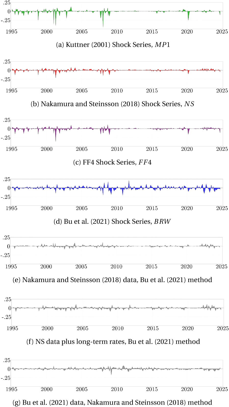
Time series of monetary shock series, January 1995 to September 2024. MP1 is the 30-min change around an FOMC announcement in the current month’s federal funds future if the FOMC announcement is in the first 23 days of the month with an adjustment or the next month’s federal funds future if the FOMC announcement is within the last seven days of the month. FF4 is the change in the three-month-ahead federal funds futures within 30 min of an FOMC announcement. NS is the first principal component of the instrument set {MP1, MP2, ED2/SF3, ED3/SF4, ED4/SF5} which is the 30-min change in these futures around an FOMC announcement. BRW is a Fama-MacBeth regression of the daily change in one- to 30-year zero-coupon Treasury yields. NS data/BRW method is a Fama-MacBeth regression of the NS data. NS plus long-term rates/BRW method is a Fama-MacBeth regression of the NS data augmented with 2-, 5-, 10-, and 30-year Treasury yields. BRW data/NS method is the first principal component of the BRW data.
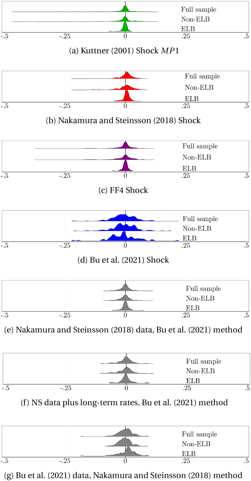
Distributions of monetary shock series, January 1995 to September 2024. MP1 is the 30-min change around an FOMC announcement in the current month’s federal funds future if the FOMC announcement is in the first 23 days of the month with an adjustment or the next month’s federal funds future if the FOMC announcement is within the last seven days of the month. FF4 is the change in the three-month-ahead federal funds futures within 30 min of an FOMC announcement. NS is the first principal component of the instrument set {MP1, MP2, ED2/SF3, ED3/SF4, ED4/SF5} which is the 30-min change in these futures around an FOMC announcement. BRW is a Fama-MacBeth regression of the daily change in one- to 30-year zero-coupon Treasury yields. NS data/BRW method is a Fama-MacBeth regression of the NS data. NS plus long-term rates/BRW method is a Fama-MacBeth regression of the NS data augmented with 2-, 5-, 10-, and 30-year Treasury yields. BRW data/NS method is the first principal component of the BRW data. The ELB is defined as December 16, 2008 to December 16, 2015 and March 15, 2020 to March 16, 2022.
Statistics of various shock series.
| Panel 1) Correlation Coefficient | Panel 2) Same Sign, % | |||||||||||||
|---|---|---|---|---|---|---|---|---|---|---|---|---|---|---|
| Shock | MP1 | NS | FF4 | BRW | NS data | NS + long | BRW data | MP1 | NS | FF4 | BRW | NS data | NS + long | BRW data |
| BRW meth. | rates data | NS meth. | BRW meth. | rates data | NS meth. | |||||||||
| BRW meth. | BRW meth. | |||||||||||||
| MP1 | 1.00 | 100 % | ||||||||||||
| NS | 0.77 | 1.00 | 47 % | 100 % | ||||||||||
| FF4 | 0.80 | 0.92 | 1.00 | 59 % | 67 % | 100 % | ||||||||
| BRW | 0.27 | 0.51 | 0.43 | 1.00 | 42 % | 65 % | 53 % | 100 % | ||||||
| NS data/BRW meth. | −0.40 | 0.22 | 0.02 | 0.28 | 1.00 | 32 % | 70 % | 52 % | 61 % | 100 % | ||||
| NS data+long rates/ BRW meth. | 0.08 | 0.62 | 0.45 | 0.49 | 0.81 | 1.00 | 39 % | 71 % | 57 % | 72 % | 82 % | 100 % | ||
| BRW data/NS meth. | −0.03 | 0.14 | 0.05 | 0.20 | 0.24 | 0.06 | 1.00 | 35 % | 57 % | 41 % | 52 % | 59 % | 53 % | 100 % |
| Shock | Panel 3) Sign at the ELB, % | |||||||||||||
| Zero | Negative | Positive | ||||||||||||
| MP1 | 38 % | 37 % | 25 % | |||||||||||
| NS | 0 % | 22 % | 78 % | |||||||||||
| FF4 | 45 % | 27 % | 27 % | |||||||||||
| BRW | 0 % | 64 % | 36 % | |||||||||||
| NS data/BRW meth. | 3 % | 45 % | 52 % | |||||||||||
| NS data + long rates/BRW meth. | 0 % | 62 % | 38 % | |||||||||||
| BRW data/NS meth. | 0 % | 32 % | 68 % | |||||||||||
-
For high-frequency monetary policy shock series, the three panels of Table 1 display their 1) correlation coefficient, 2) percentage of occurrences when the shocks have the same sign, and 3) percentage of occurrences when they are either equal to zero, positive, or negative during the ELB episodes which are defined from December 16, 2008 to December 16, 2015 and March 15, 2020 to March 16, 2022. MP1 is the 30-min change around an FOMC announcement in the current month’s federal funds future if the FOMC announcement is in the first 23 days of the month with an adjustment or the next month’s federal funds future if the FOMC announcement within the last seven days of the month. FF4 is the change in the three-month-ahead federal funds futures within 30 min of an FOMC announcement. NS is the first principal component of the instrument set {MP1, MP2, ED2/SF3, ED3/SF4, ED4/SF5} which is the 30-min change in these futures around an FOMC announcement. BRW is a Fama-MacBeth regression of the daily change in one- to 30-year zero-coupon Treasury yields. NS data/BRW method is a Fama-MacBeth regression of the NS data. NS plus long-term rates/BRW method is a Fama-MacBeth regression of the NS data augmented with 2-,5-, 10-, and 30-year Treasury yields. BRW data/NS method is the first principal component of the BRW data. The sample is January 1995 to September 2024.
Panels (1a) and (2a) show the MP1 shock series, which stands out for having some of the largest negative shocks in the sample and being close to zero throughout both ELB periods. When the federal funds rate is at the ELB – as it was from December 16, 2008 to December 16, 2015 and again from March 15, 2020 to March 16, 2022 – the FOMC has used date- or threshold-based forward guidance to communicate expected liftoff [see Carlstrom and Jacobson (2013) for an overview]. An expected liftoff date far into the future or macroeconomic indicators far from their policy thresholds has resulted in market participants perceiving a change in the federal funds rate as unlikely at the upcoming meeting. As a result, there may be either little trading in federal funds futures contracts expiring in the current or next month, or no monetary news that surprises markets. For example, panel 3 of Table 1 shows that about 40 % of ELB observations are 0 for the MP1 shock series. Moreover, the magnitudes of these shocks at the ELB are at a maximum of about five basis points.
With estimates of the MP1 shock series close to zero in the ELB periods, estimates of monetary transmission may be quite small or imprecise, leading researchers to conclude that there is no effect of monetary policy on the economy, as shown in Appendix Figures (B.23). These findings could be potentially problematic because other evidence such as the work by Swanson and Williams (2014) finds that monetary policy can have an effect at the ELB through communication that targets longer horizons as opposed to the very short horizons used to calculate the MP1 shock series.
In light of these shortcomings, the MP1 shock series has the advantage of reducing bias from either the so-called “Fed information effect” or Fed forward guidance, as noted by Paul (2020). Because either of these features could be operating in the opposite direction of direct changes in the federal funds rate, researchers concerned about contamination may find the MP1 shock series appealing.
With a 0.77 correlation coefficient, the NS shock series is similar to the MP1 shock series, as shown in panels (1b) and (2b). Like the MP1 shock series, the NS shock series is tightly distributed around zero throughout the ELB periods. In contrast to the MP1 shock series where most ELB observations were 0 or negative, 78 % of the NS shock series observations are positive at the ELB, as shown in panel 2 of Table 1. Given that the Federal Reserve has deployed record monetary stimulus at the ELB, what is the interpretation of the 78 % positive observations of the NS shock series? One could interpret unanticipated contractionary monetary news as markets expecting a larger stimulus than what was announced or implemented. Vissing-Jorgensen and Krishnamurthy (2011) note that the LSAP program known as “QE II” announced on November 3, 2010 was about $150 billion less than market expectations. However, it is unlikely that markets expected a larger stimulus in nearly four out of five announcements.
Panel 1 of Table 1 shows that with correlation coefficients of about 0.8 and 0.9, the FF4 shock series is tightly correlated with the MP1 and NS shock series, respectively. This tight correlation is not surprising given that they are all calculated over the same high-frequency intervals and rely on futures with maturities of year or less. Moreover, sometimes these series even use the same underlying data, which is especially true for MP1 in the NS instrument set. Panels (1c) and (2c) show that the distribution of the FF4 shock series narrows at the ELB like the MP1 and NS shock series, it is more centered at zero than the latter. In fact, panel 3 of Table 1 shows that 45 % of the FF4 shock observations are zero at the ELB and another 27 % are positive, which is much less than the 78 % positive observations of the NS shock. Even though the FF4 shock series avoids suggesting more contractionary monetary news than expected in a time of record stimulus, the preponderance of zero observations at the ELB suggests that FF4 may still struggle to capture monetary policy actions at the ELB.
In contrast to the other high-frequency monetary shock series previously described, panels (1d) and (2d) show that the distribution of the BRW shock series is similar across ELB and non-ELB periods. Furthermore, panel 3 of Table 1 shows that shock estimates are never zero throughout the ELB period and 64 % are negative and hence expansionary in periods of record monetary stimulus. The largest negative observations occurred when the Federal Reserve extended or announced LSAP programs in March 2009 and March 2020, respectively. We explain how both data and methods account for these findings.
Because forward guidance and LSAPs affect maturities longer than the one-year horizon of the NS instrument set, shocks series like that of BRW which are constructed from data with maturities up to 30 years should intuitively better capture the effects of these policies. However, including data on longer maturities may be insufficient as these data may be unresponsive to monetary policy on average. Figure 3a shows the responsiveness coefficients from the first step of the Fama-MacBeth regression given by equation (8). On average, Treasuries with relatively shorter maturities are more responsive to changes in the two-year Treasury on FOMC announcement days. In fact, Treasuries with maturities beyond 15 years do not have a statistically significant average responsiveness. For this reason, simply including longer-term rates in the NS instrument set via principal component analysis does not materially change the final series as shown in Appendix A.4. In fact, augmenting the NS instrument set with 2-, 5-, 10- and 30-year intraday Treasury yields results in a shock series that has a 0.92 correlation coefficient with the original NS series. We note that this correlation coefficient is higher than quite a few of the other series studied in this paper.
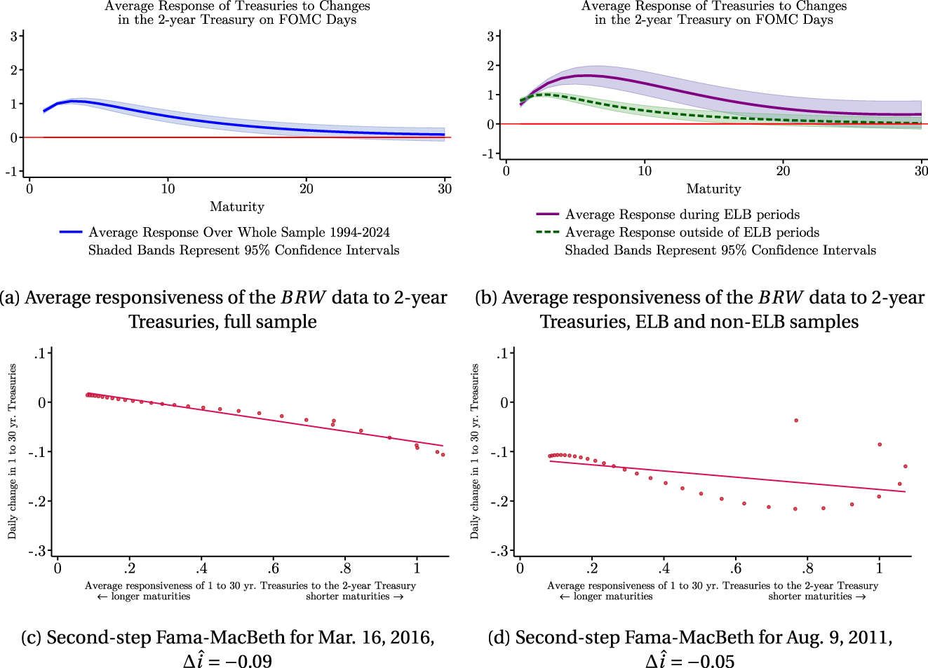
Construction of the Bu et al. (2021) shock series. Panels (a) and (b) show estimates
If long-term data alone cannot account for the differences in monetary shock series, what is the role of methods? In contrast to principal component analysis, Fama-MacBeth regression allows for the weights on underlying instruments to be time varying so that long-term rates may matter more than short-term for certain announcements and the opposite for others. By relying on the differential responsiveness of short- and long-term Treasuries, the Fama-MacBeth regression can therefore exploit information from long-term rates despite their overall average low responsiveness shown in panel (3a). The second step of the method projects the change in Treasuries for each maturity on the day of an FOMC announcement onto their average responsiveness shown in Figure 3a. If the changes across all maturities on FOMC announcement day s were equal such that
Furthermore, identifying monetary shocks via the differential responsiveness of short- and long-term rates can account for why the BRW shock series is so different than the other shock series at the ELB. Although short-term rates may be relatively unchanged due to forward guidance communicating no expected change in the federal funds rate, medium- to long-term rates may still be adjusting, especially since forward guidance and LSAPs may be targeting these rates. In fact, panel (3b) shows that medium-term rates became relatively more responsive at the ELB changing more than one-for-one relative to a change in the two-year rate. Panel (3d) confirms these differential changes by showing a particular FOMC announcement where long-term rates drop by more than short-term rates and medium-term rates are the most responsive. With roughly a −0.03 percentage point change, the one-year Treasury is the least responsive on this particular FOMC announcement during an ELB episode.
Appendices A.5 and A.6 show that the NS and BRW shock series are tightly correlated with versions constructed from real-time estimates and different normalizations, respectively. Additionally, Appendix A.7 shows versions of the BRW shock series constructed from daily changes in Treasury futures and forwards and discusses the issues therein.
2.6 Interchanging Data and Methods
To confirm that both data and methods drive the differences in the BRW shock series relative to the other shocks series studied, we follow Bu et al. (2021) and interchange data and methods of the NS and BRW shock series. Overall, we find that differences become more pronounced with the largest correlation coefficient at 0.62 and the lowest at −0.40 as shown in Table 1.
Using the NS data – intraday changes in five interest rate futures with maturities of a year or less – in the BRW Fama-MacBeth method produces shocks that have only a correlation coefficient of only about 0.2 with either of the original series, as shown in Table 1. This series has the lowest correlation coefficient in the entire table, −0.40 with the MP1 shock series.
Panels (1f) and (2f) show that the NS data with BRW method results in distributions that are similar in the ELB and non-ELB periods. By contrast, shock series based on raw data or principal component analysis have distributions that narrow at the ELB. In support of these findings, Figure 4 shows the average responsiveness of the five NS interest rate futures to the two-year constant maturity Treasury yield on FOMC days is not significantly different in ELB episodes relative to non-ELB episodes. We do note that the responsiveness of the instruments with the shortest maturities – MP1 and MP2 – is relatively lower in ELB episodes.
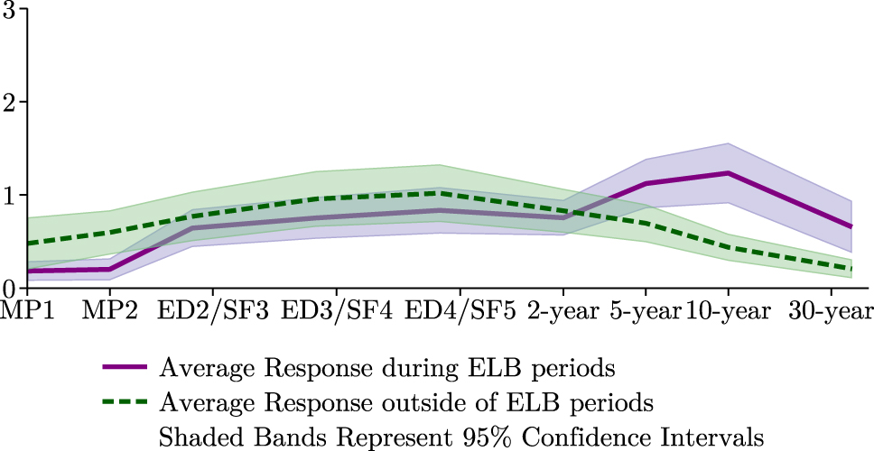
Average responsiveness of the NS data and long-term rates to two-year Treasuries on FOMC days. Estimates
Furthermore, like the original BRW shock series, the version with NS data is mostly symmetric around zero at the ELB as shown in panel (2f). Although the underlying short-term data may be left-censored, because the Fama-MacBeth regression calculates the differential variation across underlying instruments, it may not always prescribe a positive shock if all rates rise. In fact, Table 1 shows that only 52 % of observations are positive at the ELB compared with 78 % using the original principal component analysis. Finally, Figure 4 supports the findings of Swanson and Williams (2014) that monetary policy can still have effects at the ELB.
Although augmenting the NS instrument set with longer-term rates – 2-, 5-, 10-, and 30-day intraday changes in Treasuries – has little effect on the resulting shock series constructed from the NS method as shown in Appendix Figure (A.14), we now ask the question of whether this augmentation affects the BRW method. Panels 2 and 3 of Table 1 show that the series often has the same sign as other shock series studied and that the share of negative observations at the ELB is quite close to that of the original BRW series. The improved fit relative to its counterpart with only the short-term rates can likely be attributed to the increased responsiveness of long-term rates at the ELB as shown in Figure 4.
Panels (1g) and (2g) show that using the BRW data – changes in one- to 30-year zero-coupon Treasury yields – with the NS principal component analysis results in shock series that are not as small in magnitude as the other interchanged shock series shown in panels (1f) and (2f). Like the NS shock series, these interchanged shock series also have a positive mass – 68 % of observations – during the ELB periods. Because the principal component analysis is a linear combination of the underlying instruments, it will prescribe positive shock if all rates rise in response to the monetary policy announcement. Like the previously discussed interchanged shock, the shock series constructed from the BRW data with NS method has a relatively low correlation coefficient of at most 0.24 with the commonly used shocks we study.
2.7 Predictability
Because commonly used monetary shock series have been shown to be predictable and hence not entirely exogenous, we include in our discussion of shock construction predictability tests standard in the literature. Karnaukh and Vokata (2022), Sastry (2021), and Bauer and Swanson (2023) have shown that the NS shocks series is predictable by observables in the form of economic news, and Bu et al. (2021) confirm that the BRW shocks series is not. We find that shocks constructed from federal funds futures are the most likely to be predictable by economic news.
Standard tests assess if economic news predicts monetary shocks
Figure 5 shows the predictability coefficients
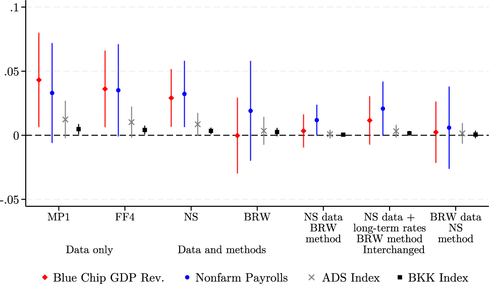
Predictability coefficients with 95 % confidence intervals. Estimate of
Finally, Figure 5 confirms that shock series constructed from long-term interest rates – the BRW shock series and its interchanged counterpart constructed from the NS principal component method – are unpredictable according to several standard tests in the literature. Because the interchanged shock series with the BRW data is also unpredictable, including long-term rates in shock construction may help ensure that high-frequency series are indeed controlling for all available pre-existing information. However, the shock series constructed only from fed funds futures – the MP1 and FF4 shock series – are only marginally predictable suggesting that predictability is most strongly associated with series constructed from the NS data. See Appendix Figure (A.18) for additional results over different sub-samples.
3 Monetary Transmission
After discussing the construction of high-frequency monetary shock series and some of their basic properties, we now explore how data and methods affect estimates of the transmission of monetary policy. We find that differences in monetary shock series are more likely to affect monetary transmission estimates from specifications that rely on forecast revisions than those from local projections or VARs. The BRW shocks series constructed from longer-term rates and the Fama-MacBeth method delivers transmission estimates that are the same sign as theoretical predictions in all specifications studied. By contrast, the shock series constructed from futures with maturities of one year or less tend have opposite-signed transmission estimates in the forecast revision specification and conventionally-signed responses in the local projections or VAR specifications. Among these shocks constructed from futures with maturities of one year or less, transmission estimates using the MP1 shock series are the closest to having the same sign across all specifications. This supports the findings of Paul (2020) that the MP1 shock series can potentially reduce bias from either the so-called “Fed information effect” or forward guidance without appealing to the add-on techniques of Miranda-Agrippino and Ricco (2021), Bauer and Swanson (2023, 2022), Jarociński and Karadi (2020), Nunes et al. (2023), Zhu (2023), and others.
3.1 Forecast Revision Specification
The monetary transmission specification of Campbell et al. (2012) and Nakamura and Steinsson (2018) estimate the response of monthly Blue Chip GDP forecast revisions to high-frequency monetary shocks. Let T index months and t higher frequencies. Following the literature,
Equation (11) can be estimated via OLS because the dependent and independent variables are not simultaneously determined. If the change in actual GDP were used instead of the change in expected GDP, this would not be the case. Because quarterly GDP statistics are the accumulation of economic output over three months, it is impossible to disentangle the output produced before an FOMC announcement – and hence pre-determined at the time of the announcement – from the output produced after the announcement. By contrast, a monthly series of GDP forecast revisions side-steps simultaneous determination by subtracting forecasts made before the announcement from those made after. The resulting forecast revision brackets the FOMC announcement and can estimate the effect of policy on perceptions about economic activity. In fact, researchers exclude monetary shock observations in the first several business days of the month to ensure that the Blue Chip survey was completed prior to an FOMC announcement, as detailed in Appendix B.
The coefficient
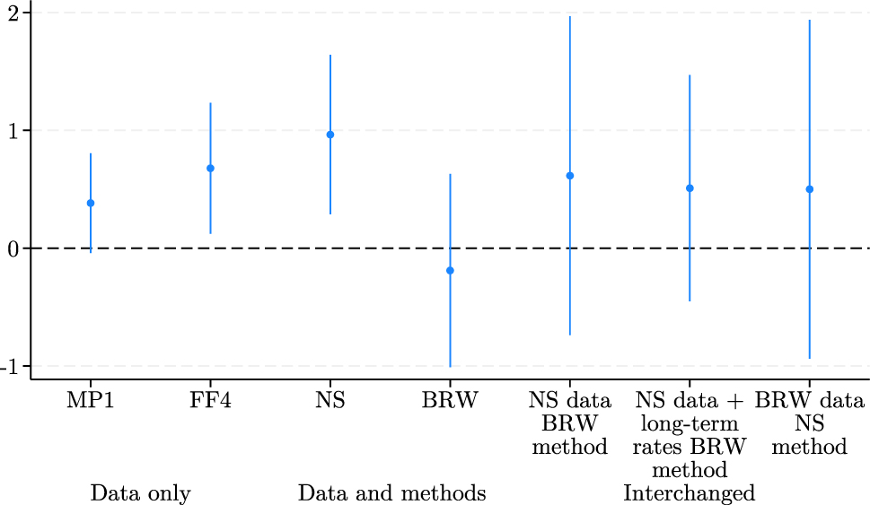
Forecast revision coefficients and 95 % confidence intervals.
The BRW and the interchanged shock series do not produce statistically significant responses suggesting that the opposite-signed response is only found in a subset of shock series. Bu et al. (2021) attribute the lack of opposite-signed response in their shock series to a combination of longer-term rates and methods. As BRW explain, if there is a differential effect of the Fed Information effect on short- and long-term rates – as shown by Hansen et al. (2019) –, adding long-term rates to the construction of monetary shock series can offset the information effect found in short-term rates. However, any information effect in short-term rates is unlikely to be offset in principal component analysis because the procedure extracts linear combinations of the underlying instruments and hence will preserve any information effect in the underlying data. Although Miranda-Agrippino and Rey (2020) and Stavrakeva and Tang (2024) find evidence of information effects in factors constructed from longer-term rates, as long as there is a differential responsiveness of short- and long-term rates, a Fama-MacBeth regression will not necessarily inherit an information effect detected in a subset of rates.
Even though the BRW shock series is the only series of the four main shock series that does not result in a positive and significant opposite-signed response, we note that the MP1 shock series of Kuttner (2001) is only on the margin of insignificance. For researchers concerned that an opposite-signed response in a shock series indicates contamination from central bank information signaling, we argue that the MP1 shock series may be an alternative to the NS shock series. Although additional procedures to the NS shock series can purge these information effects, MP1 offers the advantage of simple construction from raw data.[10] Appendix figure (B.23) confirms these findings across samples and controls.
3.2 Daily Local Projections
Although the information mismatch between central banks and private agents can account for opposite-signed responses of monetary transmission estimates, Jacobson et al. (2025) present the information mismatch between economic modelers and private agents as a complementary explanation. When response variables are observed at a lower frequency than explanatory variables – as is the case with most macroeconomic response variables – temporal aggregation bias can affect transmission estimates. Jacobson et al. (2025) show that time aggregated data can lead to earlier arriving response coefficients being magnified relative to their later arriving counterparts. When using the daily inflation series from the Billion Prices Project [Cavallo and Rigobon (2016)] as a response variable instead of the monthly official CPI, Jacobson et al. (2025) find that initial positive response coefficients are indeed magnified relative to later arriving negative coefficients. After all, the opposite-signed positive response is quite temporary, if detected at all, when the data frequencies of explanatory and response variables are better matched. Additionally, a specification with matched data frequencies does not require researchers to discard FOMC announcements that occur early in the month as is necessary for identification when data from the Blue Chip survey are used as a response variable.
After showing that the daily inflation series decently approximates the official CPI, Jacobson et al. (2025) compute local projections and find conventionally-signed responses with only a short-lived initial adverse response. Their local projection for day t + h is the following,
Where π
t+h
is daily inflation at day t + h calculated as the 30-day percentage change, z
t
is the vector of controls which are the 30 lags of daily inflation, and
Figure 7 shows the estimated impulse response functions
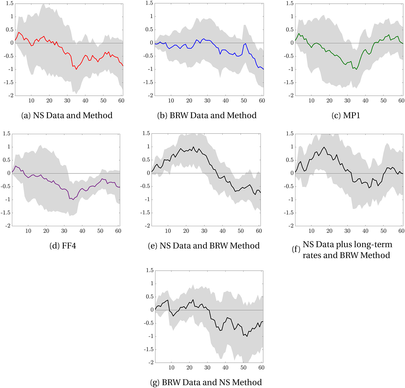
Impulse response functions of local projections to a 1 percentage point monetary shock, x-axis is days and y-axis is percentage points. Estimates of
Panels (7a) and (7b) repeat the main exercise of Jacobson et al. (2025) and show that the responses of daily inflation to the NS and BRW shock series are both conventionally-signed. Even though the transmission estimates of the forecast revision specification in Section 3.1 are positive and significant for the NS shock series, the local projection estimates are negative – and hence conventionally-signed – for a majority of the 60-day response horizon shown. The only positive – and hence opposite-signed response – is short-lived lasting about 10 days before turning negative. About 30 days after the initial impulse, the response is negative and significant. In fact, the estimated response coefficients with a negative sign are the only estimates that are statistically significant. When using the BRW shock series, the impulse responses are unambiguously negative about 60 days after a contractionary monetary shock. Unlike the NS shocks series, there are almost no estimated opposite-signed impulse response coefficients from the BRW shock series. The positive responses of the BRW shocks series are consistent with those of the forecast revision specification in Section 3.1.
Turning to the interchanged shock series shown in panels (7e) and (7f), the series constructed from the BRW method with NS data – either the original or the version augmented with long-term rates – are the only series among the seven studied in this paper that have a significant opposite-signed response. Given that the series constructed from short-term rates is tightly correlated with its counterpart constructed from short- and long-term rates, as shown in Panel 1 of Table 1, the significance of the opposite-signed response is maintained even after adding long-term rates to the instrument set. These shock series are some of the smallest in magnitude so any large swing in inflation will be ascribed to a relatively tiny impulse and result in a statistically significant response coefficient. For this reason, the shock series constructed from the NS data with the BRW method likely estimates a larger initial positive impulse response than the NS shock series constructed from its standard principal component analysis method shown in panel (7a).
Because shock series constructed from short-term rates shown in panels (7a), (7c)-(7e) all detect an initial positive impulse response, it may be tempting to ascribe opposite-signed responses to short-term rates. However, the point estimates of the impulse responses of the interchanged shock series constructed from the BRW data with the NS method shown in panel (7g) are similar to those constructed with the standard NS data and method shown in panel (7a). Methods must therefore also play a role in the similarity of coefficients observed in panels (7a), (7c)-(7d), and (7g). In the case of the interchanged shock series with the BRW data and the NS method shown in panel (7g), the error bands are wider resulting in no statistically significant response from zero. Because the distribution of the interchanged series is larger than that of the NS series over the 2008 to 2015 period, it is likely that the additional variation leads to less precise estimates.
Overall, differences in estimates of monetary transmission from local projections with matched frequencies of explanatory and response variables matter less than in the forecast revision specification with mismatched frequencies. Both data and methods account for this finding as the point estimates are quite similar for 1) the NS shock series relying on short-term futures and principal component analysis, 2) the MP1 and FF4 shock series relying on short-term futures, and 3) the long-term BRW data in the principal component analysis.
3.3 Vector Autoregression
In addition to specifications relying on forecast revisions or local projections, the effect of monetary policy on the macroeconomy is frequently estimated via a structural vector autoregression framework at a monthly frequency by using high-frequency monetary policy shock series as external instruments. Relative to the previous two specifications studied, the VAR specification has disadvantages and advantages. Unlike the daily local projection specification, VAR specifications typically have mismatched data frequencies in the form of high-frequency shocks and low-frequency response variables. On the other hand, the VAR specification has the advantage of allowing for feedback between multiple macroeconomic variables as co-movements of variables like inflation and output are well documented but absent from the specifications in Sections 3.1 and 3.2.
We use the VAR specification of Bauer and Swanson (2022) which is a variant of Gertler and Karadi (2015). The external instrument imposes a second moment restriction to identify shocks, more specifically it replaces one column of the rotation matrix with predicted values from a regression of a reduced form VAR innovation on the external instrument.[11] We focus on the VAR with external instruments as it is the dominant specification in empirical macroeconomics as noted by Miranda-Agrippino and Ricco (2023). Bauer and Swanson (2022) provide additional comparisons of the impulse responses of the NS shock and their orthogonalized variant in several VAR specifications including one where the shock series is used an internal instrument or in local projections.
Identification via an external instrument hinges on a high-frequency monetary policy shock series
Where ɛ
t
is any serially uncorrelated structural shocks driving the economy and
Since the true value of
The specification for a VAR with external instruments is given as:
Where Y T is a vector containing four monthly economic variables from January 1973 to December 2019: the log of the consumer price index (CPI), the log of industrial production (IP), the Gilchrist and Zakrajšek (2012) excess bond premium, and the two-year zero-coupon Treasury yield at a monthly frequency. Appendix D details the sources of these series, which we match the exact vintage used by Bauer and Swanson (2022) (https://www.michaeldbauer.com/files/FOMC_Bauer_Swanson.xlsx). We also note that the two-year Treasury yield is the daily change observed at the end of the month as in the previously mentioned excel spreadsheet used by Bauer and Swanson (2022). The excess bond premium controls for financial factors and the two-year Treasury is a measure of the stance of monetary policy. Although the original Gertler and Karadi (2015) specification uses the one-year Treasury, the two-year has the advantage of being less constrained at the ELB and is used by Bauer and Swanson (2022), our main comparison.
Next, B(L) is the matrix polynomial in the lag operator. Although Bauer and Swanson (2022) follow Gertler and Karadi (2015) and Ramey (2016) in using 12 lags, we shorten to 8 lags due to the sample size of our high-frequency shocks. Bauer and Swanson (2022) construct a version of the NS shock series from 1988 to 2019 while we begin our sample in 1995 which is as close to the 1994 introduction of explicit policy statements as our intraday data allows without resorting to sources we cannot replicate from intraday data on actual trades. Appendix C confirms that reducing the number of lags does not substantially change the qualitative estimates of monetary policy transmission, but does result in slightly different point estimates. As noted by Ramey (2016), these types of specifications are highly sensitive to the underlying data sample and may therefore differ from the original Gertler and Karadi (2015) estimates which are from 1991 to 2012.
Finally,
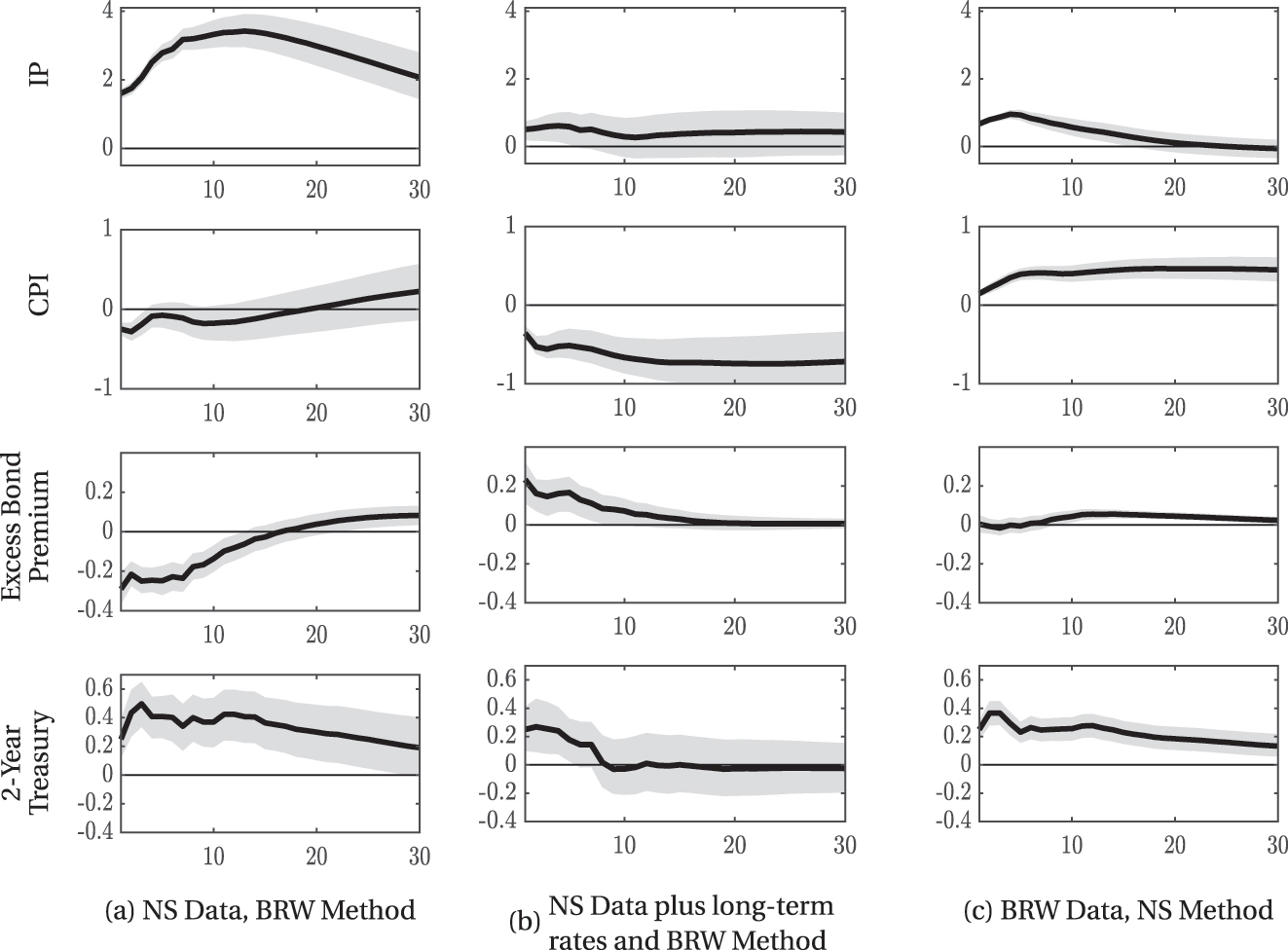
Figure 8 plots impulse responses from equation (13) obtained via the Canova and Ferroni (2022) toolbox with 68 % error bands and 20,000 draws. For the four main shock series studied in this paper, the impulse responses to a 25 basis point monetary shock are qualitatively in line with macroeconomic theory and similar in sign and shape. The response of the two-year Treasury shown in the bottom row of each panel rises on impact and is normalized so that its initial response is 25 basis points. After initially rising, the two-year Treasury decreases and returns to zero about 10 months after the initial impulse. The excess bond premium displayed in the third row rises on impact to about 0.2–0.4 percentage point in all series shown and then declines towards zero.
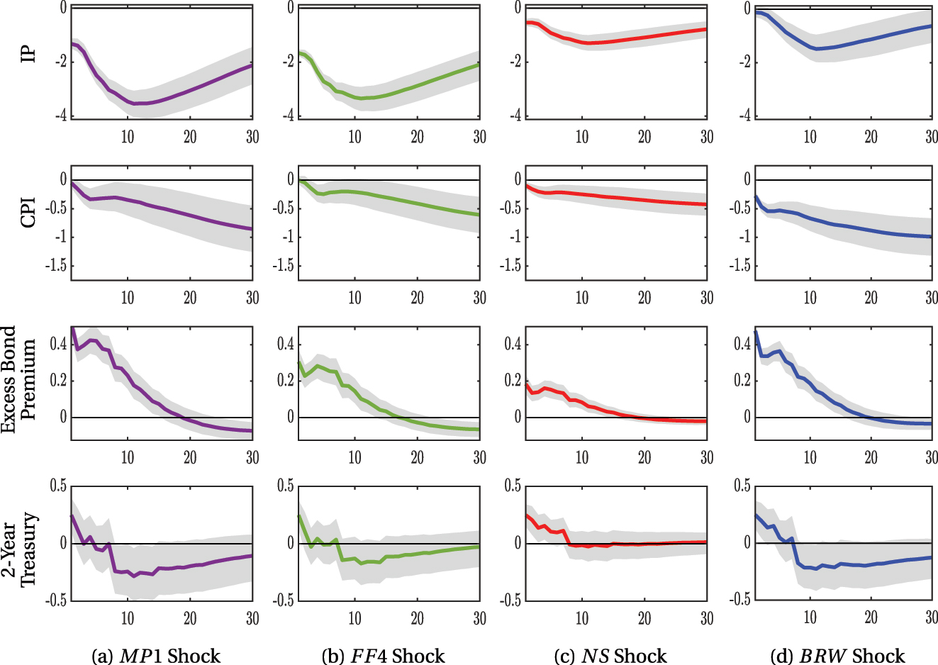
Impulse responses to a 25 basis point monetary shock, x-axis is months and y-axis is percentage points. Impulse responses are estimates from equation (13)
The impulse responses of both industrial production and CPI shown in rows one and two of Figure 8, respectively, to a contractionary monetary shock are significantly negative – as standard New Keynesian theory predicts. We find no evidence of opposite-signed responses in CPI or industrial production as was found in the forecast revision specification in Section 3.1 or elsewhere in the literature. Differences in point estimates among the four shock series are only in magnitude rather than in sign. The responses of industrial production shown in the first row are the largest for the MP1 and FF4 shock series shown in panels (8a) and (8b), respectively. The responses of CPI shown in the second row have similar interpretation to the responses for industrial production. All CPI responses are statistically significant and negative with those of the MP1 and FF4 shocks in panels (8a) and (8b), respectively, being the largest in magnitude. However, the response of CPI to the BRW shock series in panel (8d) has an initial response that is largest in magnitude the CPI.
The differences between the NS and BRW shock series are relatively minor with the exception of the response of the excess bond premium, which can be explained by BRW’s shock construction including the longer-end of the yield curve. Inference with respect to other variables (CPI, industrial production and two-year Treasury) would not be substantially different between the BRW and NS series. Conversely, the MP1 and FF4 shock series show much larger responses of the CPI.
Both the similarity of impulse responses and the conventionally-signed estimates in Figure 8 could suggest that differences in monetary shock series are negligible when estimating monetary transmission in a VAR with external instruments. However, Figure 9 shows that the impulse responses of the interchanged shock series are quite different than their counterparts shown in Figure 8 as the interchanged shock series often estimate opposite-signed responses. Panel (9b) shows that the impulse responses to the shock series constructed from the NS instrument set augmented with long-term rates in the BRW method is somewhat of an exception as some of the point estimates are conventionally-signed like those of the main shock series shown in Figure 8. However, given the opposite-signed response to industrial production we still caution that interchanging data and methods can drastically change the inference. Together, these findings suggest that even though differences in monetary shock series can affect VAR estimates, the effects of these differences range from quantitatively small when comparing the four main shock series studied to qualitatively large when examining combinations of data and methods. An econometrician must proceed cautiously as inference is not robust to all modern constructions of monetary policy shock series. Appendix Table 3 displays the first-stage F-statistics.
Impulse response to a 25 basis point monetary shock, x-axis is months and y-axis is percentage points. Impulse responses are estimates from equation (13)
First-stage F-statistics.
| Series name | F-stat | Robust F-stat |
|---|---|---|
| MP1 | 0.77 | 0.54 |
| FF4 | 0.78 | 0.31 |
| NS | 1.88 | 1.23 |
| BRW | 0.94 | 0.87 |
| NS data, BRW method | 0.58 | 0.44 |
| NS data plus long-term rates, BRW method | 0.55 | 0.82 |
| BRW data, NS method | 2.54 | 4.18 |
-
Estimates from equation (13)
Although Section 2 documents differences in several commonly used monetary policy shocks, we find that the effect of these differences on estimates of monetary transmission can be small depending on the specification used. Specifications like the daily local projections and VAR with external instruments in Sections 3.2 And 3.3, respectively, are more similar in terms of signs and magnitudes of estimates than the forecast revision specification in Section 3.1.
4 Conclusions
Because monetary policy simultaneously affects and responds to economic conditions, identifying exogenous variation is an ongoing challenge for researchers. Since at least Kuttner (2001), high-frequency environments have proven useful for overcoming these challenges by extracting unanticipated market surprises that control for all available information prior to an FOMC announcement. To construct monetary shock series, researchers separate monetary news from their non-monetary counterparts by calculating the change in asset prices minutes after an FOMC announcement relative to the prices observed just before.
Although various high-frequency monetary shock series rely on similar narrow time windows around the same monetary policy announcements, we document that their signs and magnitudes are quite different for the United States. Furthermore, these differences are starkest when the federal funds rate is at its effective lower bound and the Federal Reserve has typically deployed an expansive toolkit. Because underlying data and statistical methods can differ in shock construction, we ask what drives differences in monetary shock series. We find that data on long-term rates can contribute to differences, but methods are also important. Because the Federal Reserve’s 21st-century monetary policy toolkit can affect short- and long-term rates, long-term rates can capture additional information. However, long-term rates may be, on average, relatively unresponsive to monetary policy. Therefore, methods like the Bu et al. (2021) Fama-MacBeth regression that rely on the differential responsiveness of short and long-term rates are more effective at extracting additional information from long-term rates.
After constructing commonly used monetary shock series from raw data to highlight the choices faced by researchers, we analyze if differences in shock series matter for inference. We find that estimates of monetary transmission from local projections and VARs are more similar across shock series than their counterparts estimated via forecast revisions. In fact, some of the shock series with the simplest data and methods – the Bu et al. (2021) BRW and Kuttner (2001) MP1 shock series – are the most likely to deliver estimates of monetary transmission that are consistent with predictions from New Keynesian models across several different specifications.
A Appendix: Shock Construction
All intraday data are from CME Group Inc. DataMine (https://datamine.cmegroup.com/) at the Federal Reserve Board which is available starting in 1995. Although it may be possible to construct monetary policy shock series back to 1994 or 1988 with other data sources, we prefer to truncate our data sample than merge it with data we are unable to replicate and verify on a trade-by-trade basis.
Our underlying data closely match those of Acosta (2023) and Acosta et al. (2024) which are similarly constructed from tick data. Compared to the original series available on the authors’ websites of Nakamura and Steinsson (2018) and Bu et al. (2021), our series have a 0.99 and a 0.99 correlation, respectively. The correlation is 0.98 and 0.97 for the MP1 and FF4 series, respectively, available from Gürkaynak et al. (2023) at (http://www.bilkent.edu.tr/ ∼ refet/replication_GKL.zip).
Our January 1995 to September 2024 sample includes 244 FOMC announcements, 7 of which are unscheduled.[13] We drop intermeeting announcements that are notational votes or about topics not directly related to monetary policy actions such as: swap lines, financial crisis facilities, the debt ceiling, the monetary policy framework review, foreign economic crises, the outbreak of war in Iraq, or swap lines. We drop the announcements following 9/11 (as is common in the literature) and drop the March 15, 2020 announcement that occurred on a Sunday which precludes the availability of trades.
A.1 Appendix: Asset Price Details
Federal Funds Futures are futures contracts traded on the Chicago Mercantile Exchange since 1988. The contract index, following the International Monetary Market (IMM) convention, is priced as f f j = 100 − R, where R is the arithmetic average of the daily effective federal funds rates during the contract month j for j > 0. For example, a price quote of 95.75 is equivalent to an average daily rate of 4.25 over the course of the month in which the contract matures. The federal funds futures contract unit is $4,167 × contract index with a tick size of one-quarter of one basis point (0.0025), or $10.4175 (0.0025 × $4, 167) for the nearest month’s contract and one-half of one basis point (0.005), or $20.835 per contract for all other months. Contracts are monthly listed for 60 consecutive months and are traded Sunday through Friday from 6:00 pm to 5:00 pm EST. The effective federal funds rate is calculated as a volume-weighted median of overnight federal funds transactions and is reported by the Federal Reserve Bank of New York on the next business day by 9 A.M. Eastern Time in the FR 2420 Report of Selected Money Market Rates. Expiring contracts are cash settled against the average daily federal funds overnight rate for the delivery month, rounded to the nearest one-tenth of one basis point with final settlement occurring on the first business day following the last trading day.
Following the literature, we measure the change in federal funds rate futures around monetary policy announcements in month s and time t as
Eurodollar Futures were quarterly futures contracts traded on the Chicago Mercantile Exchange from 1981 to April of 2023. Eurodollars is a generic term to describe U.S. dollar-denominated deposits at foreign banks or at the overseas branches of American banks that are outside of the purview of the U.S. financial regulatory framework. Prior to their discontinuation in April of 2023, eurodollar futures had a payout at expiration based on the three-month maturity U.S. dollar London Inter-Bank Offer Rate (LIBOR). The pricing of eurodollar futures follows the same convention as the fed funds futures: 100-index, with a contract unit of $2,500 × contract index. Tick size was one-quarter of one basis point (0.0025 = $6.25 per contract) in the nearest expiring contract month and one-half of one basis point (0.005 = $12.50 per contract) in all other contract months. Contracts were quarterly listed, maturing during the months of March, June, September, or December, plus four serial months and a spot month, extending out ten years. Contracts were settled in cash on the 2nd London bank business day prior to the 3rd Wednesday of the contract month, and here we follow the timing convention of Nakamura and Steinsson (2018) in that new quarters begin on the 15th day of the month of the preceding quarter (e.g., 2023:Q1 would begin on December 15, 2022). Convergence to a final settlement price was forced by “randomly” polling twelve banks actively participating in the LIBOR market during the last 90 min of trade and at close. Of course our use of quotation marks in “randomly” refers to the price fixing that had taken place in this market. Highest and lowest price quotes were dropped and the arithmetic average of the remaining quotes determined final settlement.
Eurodollar futures were one of the most actively traded futures contracts in the world as measured by open interest. The extended duration of the contract, relative to fed funds futures, is the primary benefit of using eurodollar futures to identify exogenous variation in monetary policy. The duration at which the fed funds futures market liquidity begins to dry up is where eurodollar futures were most heavily traded. Gürkaynak et al. 2007b) confirm that the combination of federal funds and eurodollar futures are the best financial instruments to predict changes in the federal funds rate one year ahead.
SOFR Futures based on the Secured Overnight Financing Rate (SOFR) have successfully replaced eurodollar futures on the Chicago Mercantile Exchange. The SOFR rate is based on the cost to borrow USD overnight using Treasury securities as collateral. Because SOFR futures are designed to replace eurodollar futures, they can be spliced into shock construction when they are available. Acosta et al. (2024) recommend January 2022 as a start date for SOFR futures, but also note that the choice of start date has little effect on the construction of final estimates.
We measure the change in eurodollar/SOFR futures around monetary policy announcement in quarter q at time t as:
US Treasury securities have maturities of one to 30 years and are so well known that they do not require a thorough description. Because Hansen et al. (2019) and Hanson and Stein (2015) document that Treasuries react to monetary policy announcements with varying degrees of responsiveness depending on the maturity, Treasuries are well suited to capture monetary surprises. Bu et al. (2021) use the daily change in zero-coupon Treasury yields to construct a high-frequency monetary shock series. The zero-coupon yields, as calculated by Gürkaynak et al. 2007a)(https://www.federalreserve.gov/pubs/feds/2006/200628/200628abs.html), harmonize Treasury yields of various maturities to reflect what the discount would be if interest payments were not made until maturity. We measure the change in Treasury yields around each monetary policy announcement s as
A.2 Appendix: Shock Construction Details
This Appendix describes shock construction details.
Kuttner (2001), MP1
Kuttner (2001) notes that because the settlement prices of the federal funds futures are based on the average of the effective overnight federal funds rate in month s rather than the federal funds rate on a specific day, one must correct for the time averaging and scale by the inverse of the share of days remaining in the month after an FOMC announcement occurs. For this reason,
Nakamura and Steinsson (2018) , N S
The next scheduled FOMC meeting used to calculate MP2 may be in the next month or up to two months after the current announcement, as shown by column 1 of Appendix Table 2. Column 2 shows that the futures used to calculate MP2 may be as far as three months after the current announcement because of the convention of using the following month’s future when an FOMC announcement is in the final seven days of a month. Overall, the table shows that most of the meetings used to calculate MP2 are either one or two months ahead such that j = 2, 3. As noted previously, limited trading in federal funds futures at horizons beyond four months has led researchers to rely on eurodollar futures to capture the remaining horizons of the first year of the term structure. Because eurodollar/SOFR futures are quarterly, q indexes the quarter of the current FOMC announcement. For example, if q = 2014:Q1, ED2/SF3, ED3/SF4, and ED4/SF5 in equations (A.3)–(A.5) represent contracts expiring in 2014:Q2, 2014:Q3, and 2014:Q4, respectively.
Months ahead of the next scheduled FOMC meeting.
| Future | Next scheduled FOMC announcement | ||||
|---|---|---|---|---|---|
| (1) | (2) | ||||
| Percent | Number | Percent MP2 | Number MP2 | ||
| FF1 | In current month | 1 % | 3 | 0 % | 0 |
| FF2 | 1 month ahead | 50 % | 122 | 22 % | 53 |
| FF3 | 2 months ahead | 49 % | 119 | 76 % | 185 |
| FF4 | 3 months ahead | 0 % | 0 | 2 % | 6 |
| Total | 244 | 244 | |||
-
The next scheduled FOMC meeting occurs in the current month when an unscheduled meeting occurs before a scheduled meeting as happened in January 2008 when there was an unscheduled conference call on January 21st that announced an interest rate cut and a scheduled announcement on January 30, 2008. 1 month ahead implies that the next scheduled meeting is the month following that of the current FOMC meeting and 2 months ahead implies two months, etc. The futures used in MP2 (column 2) may differ from those in column 1 because the future for the month following that of the next scheduled FOMC announcement is used when that announcement is scheduled in the final seven days of the month. For example, the announcement following the March 18, 2015 announcement is on April 29, 2015. Because April 29 is in the last seven days of April, FF3 instead of FF2 would be used to represent the next month’s FOMC announcement. The sample is from January 1995 to September 2024.
The first principal component of the Gürkaynak et al. (2005)/ Nakamura and Steinsson (2018) instrument set updated with SOFR futures {MP1, MP2, ED2/SF3, ED3/SF4, ED4/SF5} explains about 80 % of the variation. The estimated loadings are relatively equal, which likely stems from all futures in the instrument set having maturities of less than a year and moving in lock-step. Otherwise, one could expect a particular instrument to be associated with a higher loading if its movements were typically outliers relative to the others.
A final step in the construction of the NS shock series consists of re-scaling the first principal component of equations (A.1)–(A.5) into interpretable units. Unlike the MP1 shock series that is simply a percentage point surprise in the federal funds rate, a principal component is not so straightforward. Following Nakamura and Steinsson (2018), we use the fitted value from the regression of the daily change in the one-year zero-coupon Treasury yield on the first principal component. The coefficients from this regression are quite small with a value of about 0.02 for the slope and zero for the constant.
Gertler and Karadi (2015), FF4
Because the three-month-ahead horizon of FF4 covers the next scheduled FOMC announcement as shown by Appendix Table 2, the FF4 shock series can be interpreted as capturing the effects of both federal funds rate decisions and forward guidance in a single instrument. Appendix Figure (A.10) shows how FF4 covers the next FOMC announcement and can cover up to three FOMC announcements which is the case about 10 % of the time. Furthermore, Appendix Table 2 shows that FF4 is occasionally used in the calculation of MP2 and therefore contained in the NS instrument set.
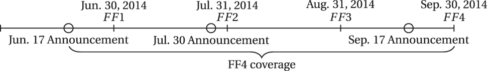
Timing of futures and FOMC announcements.
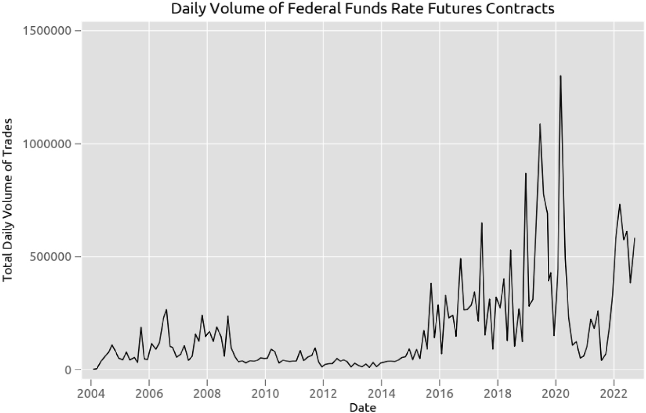
Total daily number of trades of federal funds futures contracts. Source: CME Group Inc.
A.3 Appendix: Windows for Sourcing Intraday Trades
The MP1, FF4, and NS shock series are all constructed from intraday futures data observed minutes before a FOMC announcement and minutes after. However, due to the availability of trades, the minutes “before” and “after” may not be as uniform as researchers would like.
Following Gürkaynak et al. 2007b; Nakamura and Steinsson 2018), researchers construct intraday shocks by selecting trades of federal funds or eurodollar futures 10 min before an FOMC announcement and 20 min after. However, there are not always trades at these exact times. Typically, trades that take place less than 10 min before an announcement or 20 min after are not considered. Trades that take place more than 10 min before an announcement are considered and researchers select the closest possible trade since 4:00 P.M. on the preceding day – the time when after-hours trading officially begins. Similarly, if there is no trade exactly 20 min after an FOMC announcement the closest trade is taken, up to noon on the subsequent day. If no suitable trades before or after the monetary policy announcement exist within these conditions, the change is set to 0.
Appendix Figures (A.12) and (A.13) show the size of the time windows around FOMC announcements for each of the five futures in the NS instrument set and the FF4 series.
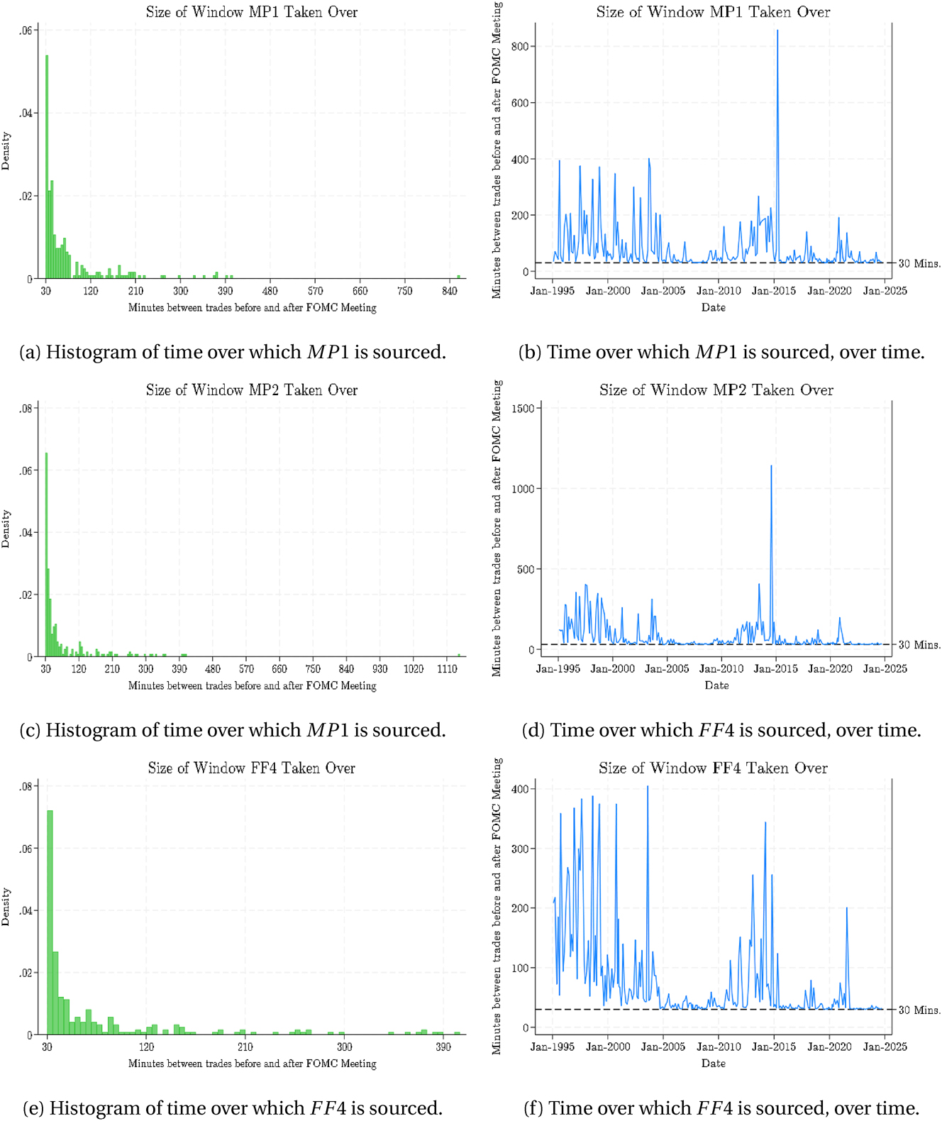
Time windows around FOMC announcements for federal funds rate futures.
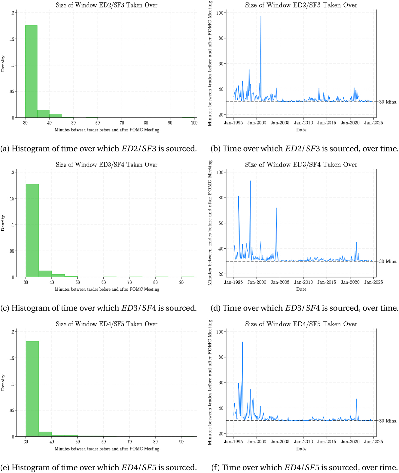
Time windows around FOMC announcements for eurodollar futures. SOFR futures replace eurodollar futures starting in January 2022.
Appendix Figure (A.12) shows that trades in federal funds futures markets are often not available in exact 30-min windows around FOMC announcements. While a large share of available intraday trades are within an hour of an announcement, it is not uncommon for intraday windows to be several hours long. Moreover, wider windows are particularly prevalent pre-2005 and during ELB periods. Appendix Figure (A.13) reveals a similar, although less extreme, phenomenon in the availability of trades in eurodollar/SOFR futures.
A.4 Appendix: Nakamura and Steinsson (2018) shock Series with Treasury yields in the Instrument set
Appendix Figure (A.14) shows the original NS shock series along with a version that is augmented to include 2-, 5-, 10-, and 30-year Treasury yields in the instrument set. Including the long-term rates has little effect on the resulting series because monetary policy is unresponsive to longer-term rates on average.
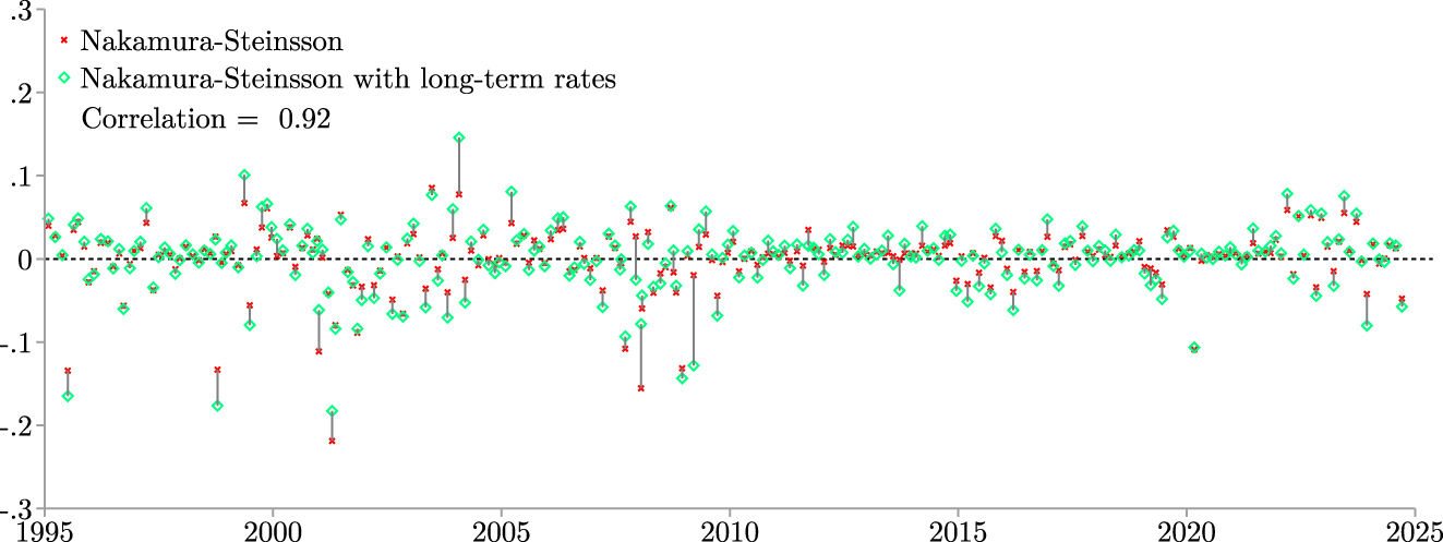
Nakamura and Steinsson (2018) series with and without long-term rates. Monetary shock series are calculated from January 1995 to September 2024. NS is the first principal component of the instrument set {MP1, MP2, ED2/SF3, ED3/SF4, ED4/SF5} which is the 30-min change in these futures around an FOMC announcement. NS plus long-term rates augments the original instrument set with 2-, 5-, 10-, and 30-year Treasury yields.
A.5 Appendix: Real Time Estimates
The MP1 and FF4 shock series are based on changes in raw data, with MP1 having a small scalar multiple adjustment based on the days remaining in the month of a meeting. By contrast, the Nakamura and Steinsson (2018) and Bu et al. (2021) shock series are constructed from statistical procedures (principal component analysis and Fama-MacBeth regression, respectively), which raise concerns of discrepancies in shock estimates compared to real-time versions.
We compare these shock series to their so-called “real-time” counterparts – that is, shocks for which the nth monetary policy announcement’s shock is calculated using data for only the first n monetary policy announcements. We begin these real-time estimates at the 30th meeting in our sample so that the statistical procedures have sufficient observations. Appendix Figure (A.15) shows that, overall, there is not much difference between the real-time shock series and their full sample counterparts. Both the NS and BRW shock series have a correlation close to one with their real-time counterparts. Some real-time observations, particularly for the BRW shock series near the onset of the Great Financial Crisis, can substantially differ, but these are not many. Overall, these give us reassurance that it does not matter much if a researcher uses shocks constructed as real-time estimates or shocks constructed using the entire sample.
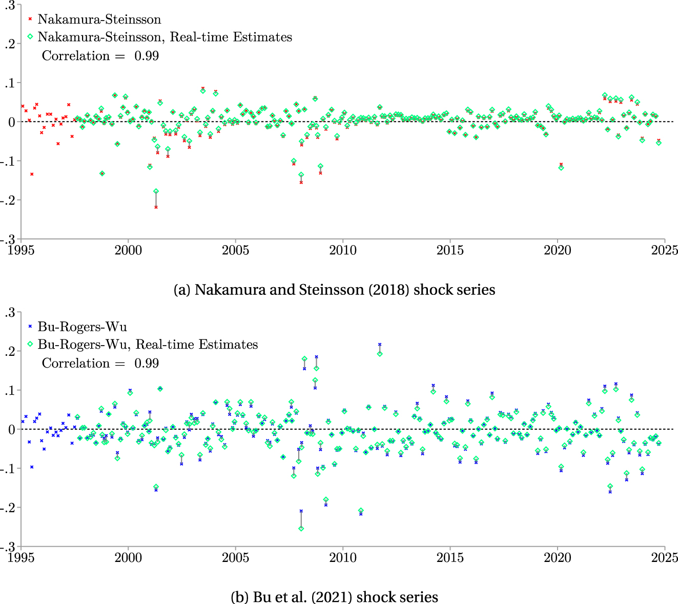
Real-time versions of Nakamura and Steinsson (2018) and Bu et al. (2021) series. Monetary shock series are calculated from January 1995 to September 2024. Real-time estimates calculate the shocks from the first 30 FOMC announcements and then update the estimates recursively. From the 31st estimate onward, each shock observation only contains information that was available at the time of the FOMC announcement. NS is the first principal component of the instrument set {MP1, MP2, ED2/SF3, ED3/SF4, ED4/SF5} which is the 30-min change in these futures around an FOMC announcement. BRW is a Fama-MacBeth regression of the daily change in one- to 30-year zero-coupon Treasury yields.
A.6 Appendix: Scalings of Shocks
The methodologies of both the Bu et al. (2021) and Nakamura and Steinsson (2018) shock series require scaling for interpretation. Both shock series scale to Treasury yields: the Nakamura and Steinsson (2018) shock series to the one-year zero-coupon Treasury yield and the Bu et al. (2021) shock series to the two-year constant maturity Treasury yield. To test if the choice of scaling matters, we use different maturities.
Panel (A.16a) shows that using the change in the two-year zero-coupon Treasury yield instead of the one-year makes little difference for the Nakamura and Steinsson (2018) shock series: both versions of the series share the same sign 100 % of the time and their correlation coefficient is a perfect 1.00. This nearly perfect correlation stems from the final step of the shock construction where one scales the first principal component by the coefficient estimate of the scaling variable on the first principal component.
Panel (A.16b) similarly shows that scaling makes little difference for the Bu et al. (2021) shock series. The correlation coefficient between the shock series constructed from the original two-year constant maturity scaling and its counterpart constructed from the one-year is 0.97. When there is some difference in estimates, it is because the scaling variable used in the Bu et al. (2021) Fama-MacBeth regression is used in both the beginning and end of shock construction. While the choice of scaling at the end is simply a means to convert a shock series to interpretable units in the same manner as in the construction of the Nakamura and Steinsson (2018) shock series, the choice of scaling at the beginning could be less innocuous. In the first step of the Fama-MacBeth regression, the choice of scaling variable is also a choice of normalization for which to assess average responsiveness. However, as Appendix Figure (A.16b) demonstrates, this choice ultimately makes little difference in the constructed monetary shock series.
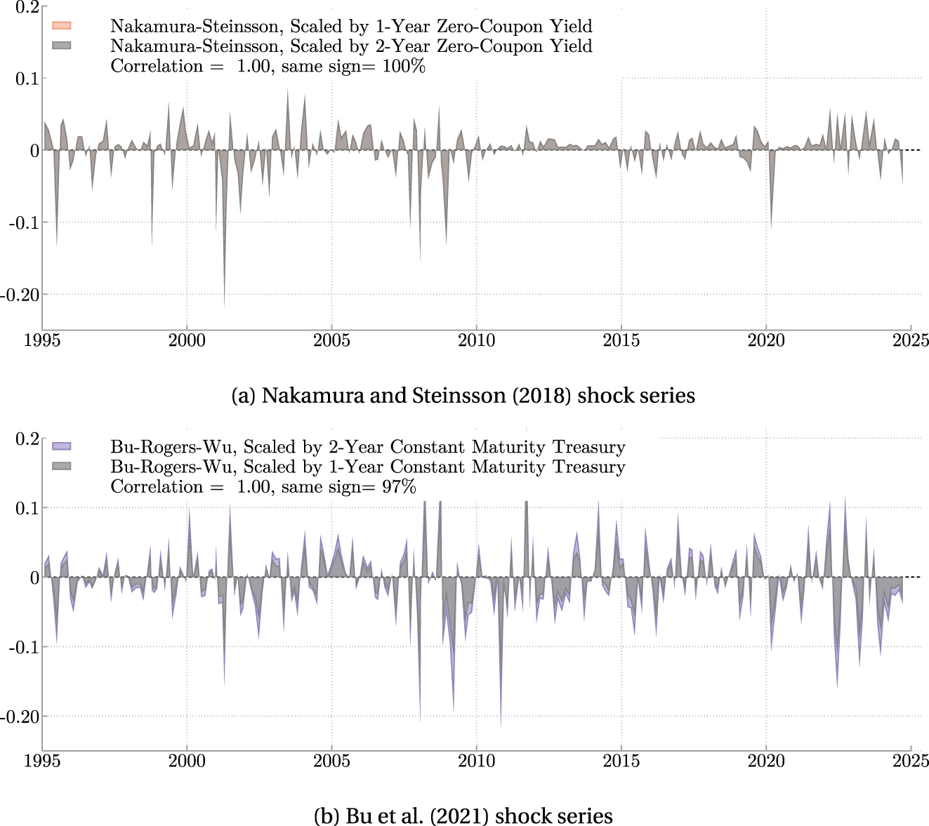
Monetary shock series under different scaling assumptions. Monetary shock series are calculated from January 1995 to September 2024. NS is the first principal component of the instrument set {MP1, MP2, ED2/SF3, ED3/SF4, ED4/SF5} which is the 30-min change in these futures around an FOMC announcement. BRW is a Fama-MacBeth regression of the daily change in one- to 30-year zero-coupon Treasury yields.
A.7 Appendix: Alternative Treasury Yield Calculations
The BRW shock series is constructed from zero-coupon Treasury yields available via Gürkaynak et al. 2007a) (https://www.federalreserve.gov/pubs/feds/2006/200628/200628abs.html). Appendix Figure (A.17) shows alternative series constructed from alternative underlying Treasuries data. The series shown in panel (A.17a) uses one- to 30-year forward rates of Treasuries also available via Gürkaynak et al. 2007a) and panel (A.17b) uses 2-, 5-, 10-, and 30-year yields of Treasury futures available via Bloomberg per security.
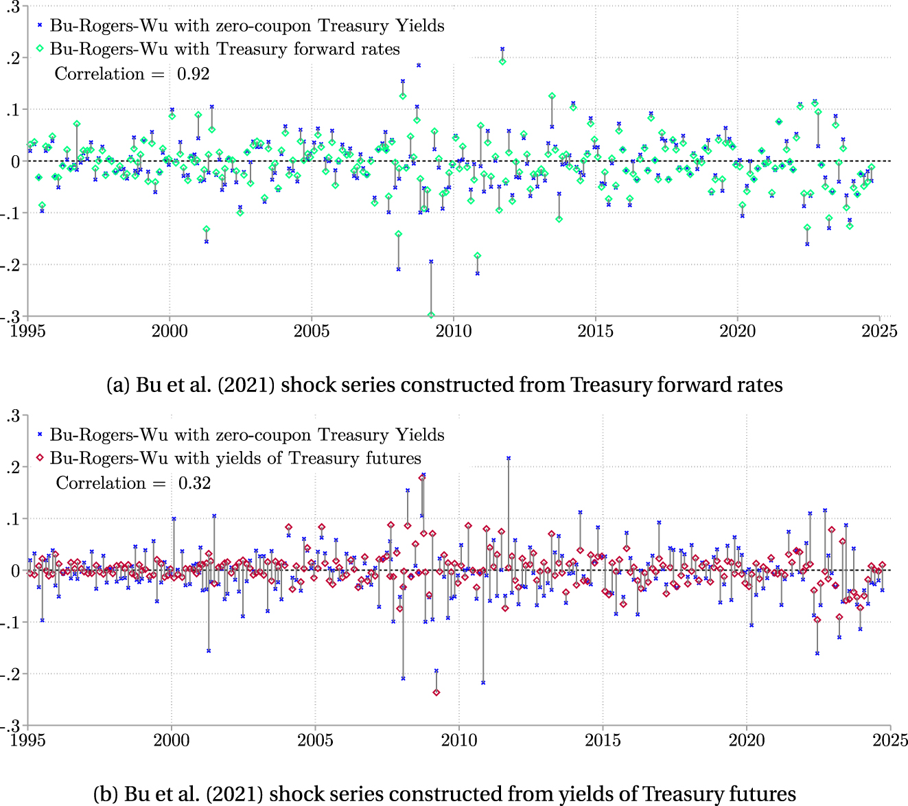
Bu et al. (2021) shock series under different Treasury data. BRW is a Fama-MacBeth regression of the daily change in one- to 30-year zero-coupon Treasury yields. BRW with Treasury forward rates is a Fama-MacBeth regression of the daily change in one- to 30-year forward Treasury rates available via Gürkaynak et al. 2007a). BRW with yields of Treasury futures is a Fama-MacBeth regression of the daily change in 2-, 5-, 10-, and 30-year yields of Treasury futures available via Bloomberg per security.
The correlation of the series based on zero-coupon yields and that based on forward rates is about 0.9, as shown by panel (A.17a). The tight correlation is not surprising given that the yields can be interpreted as the average of the forward rates, as explained by Gürkaynak et al. 2007a). However, differences emerge in the maturities because the near-term rates are more affected by monetary policy and cyclical variables than their long-term counterparts. The correlation of the underlying daily changes on days of FOMC announcements is about 0.9 for two- and five-year maturities and only 0.75 and 0.65 for 10- and 30-year maturities, respectively.
The correlation of the series based on zero-coupon yields and that based on yields of Treasury futures is only about 0.32 and can likely be attributed to a shortage of liquidity in the near-term maturities, particularly the two-year.[15] Daily changes in the 10- and 30-year Treasury futures on days of FOMC announcements are tightly correlated with their zero-coupon counterparts such that the correlation coefficients are around 0.9 and 0.75, respectively. However, the correlation coefficients are only around 0.25 for the two- and five-year maturities. Given the low liquidity throughout the early part of the sample, we recommend using either zero-coupon yields or forward rates instead of actual Treasury futures.
A.8 Appendix: Predictability Regressions
Because high-frequency monetary policy shock series should be exogenous, it is clearly desirable that the series are not significantly associated with observable macroeconomic news. Following the literature, we test if the seven series studied in this paper are predictable by economic news. More specifically, we use as measures of economic news the monthly releases of one-quarter-ahead Blue Chip Economic Indicators output growth revisions, the business conditions index of Aruoba et al. (2009) (ADS Index), the Chicago Fed Big Data Business Cycle Indicator of Brave et al. (2019), or the monthly change in nonfarm payrolls. See Appendix D for sources of these series.
The predictability regressions are estimated via OLS with Huber-White robust standard errors, where the dependent variable is the monetary shock series being tested and the independent variable is the macroeconomic news that may be a predictor of the shock. Each monetary shock series is aggregated to a monthly frequency via summation and months without a monetary policy announcement are set to zero.
Following the literature, we ensure that news pre-dates FOMC announcements. The Blue Chip one-quarter-ahead output growth revisions and the nonfarm payrolls releases are not released on the first of the month, so for specifications using either as an independent variable must exclude months in which there is a monetary policy announcement before the release of the independent variable. For specifications where the independent variable is Blue Chip one-quarter-ahead output growth revisions, we exclude months before December 1, 2000 in which a monetary policy announcement is within the first four business days of the month and we drop months after December 1, 2000 for which a monetary policy announcement is within the first three business days of the month. For specifications where the independent variable is the monthly change in nonfarm payrolls, we exclude months in which a monetary policy announcement occurs within the first seven days of the month and within the first business week of the month (Appendix Figures (A.18–A22)).
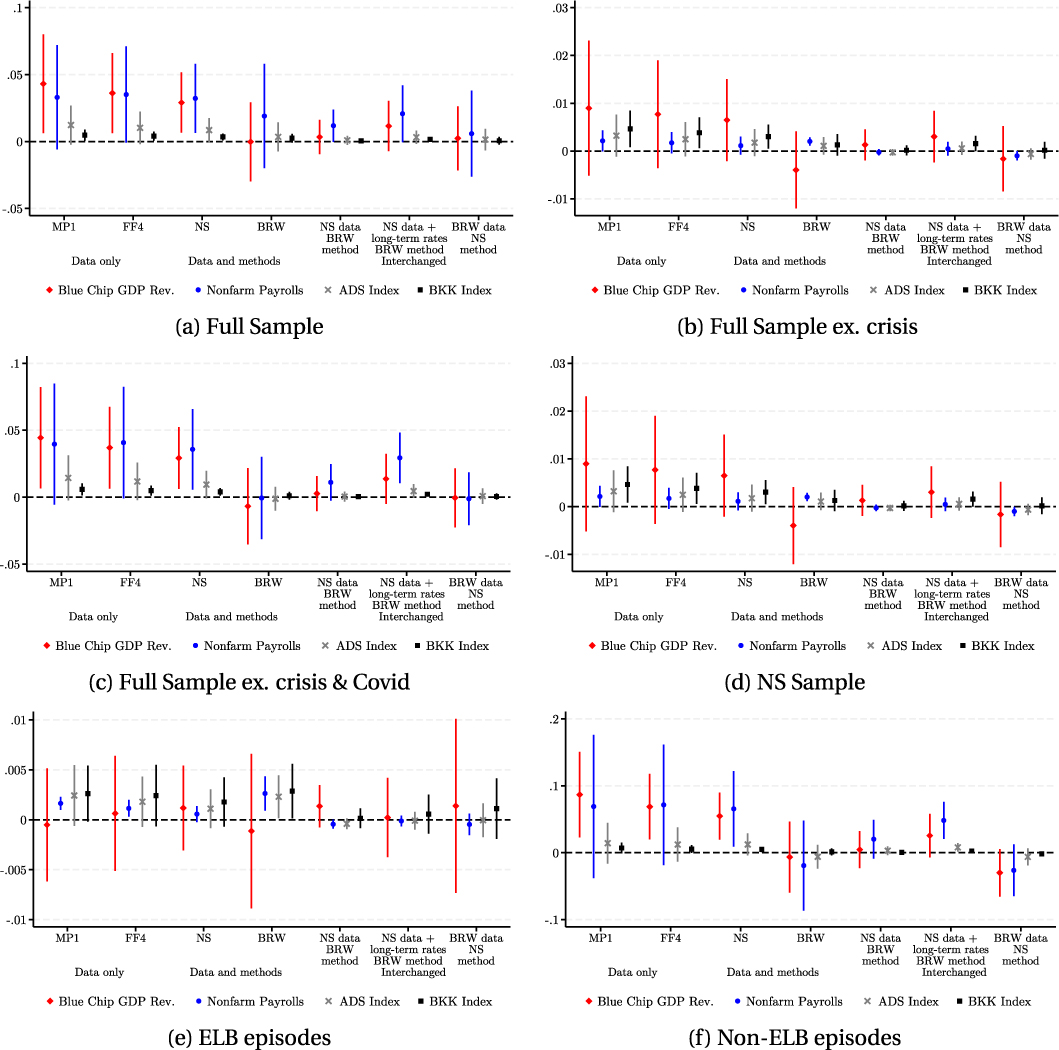
Predictability coefficients with 95 % confidence intervals. Estimate of
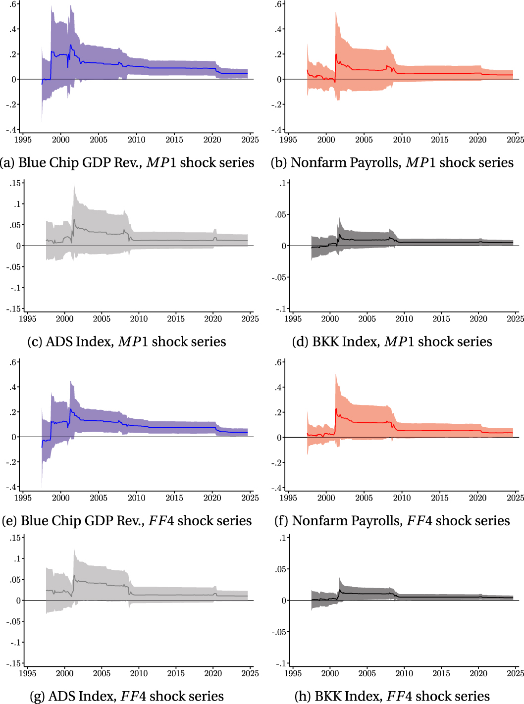
Predictability coefficients with 95 % confidence intervals. Real-Time Estimate of
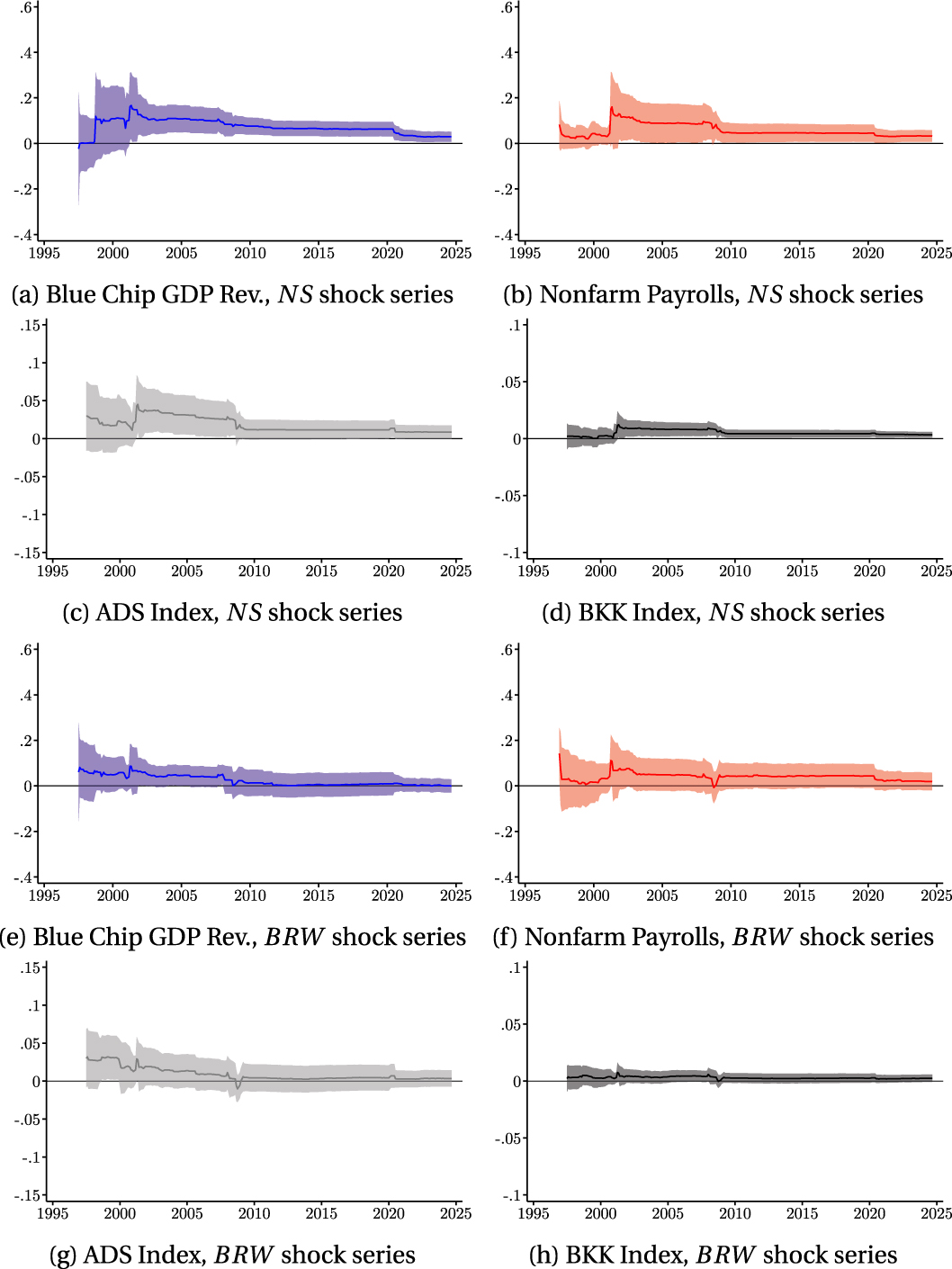
Predictability coefficients with 95 % confidence intervals. Real-Time Estimate of
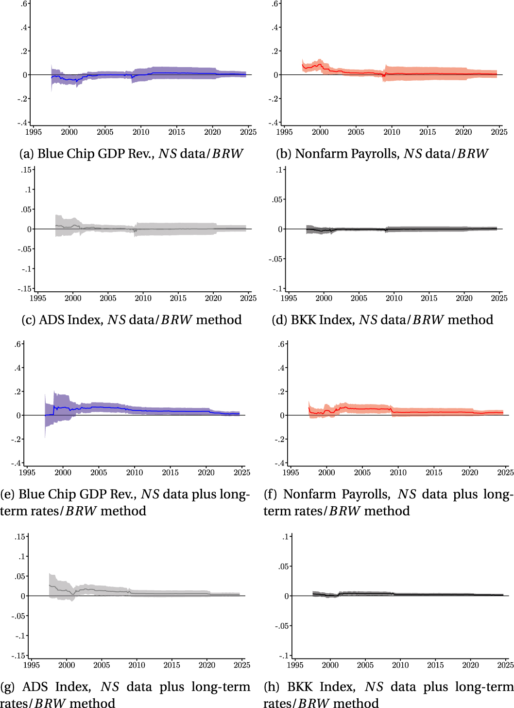
Predictability coefficients with 95 % confidence intervals. Real-Time Estimate of
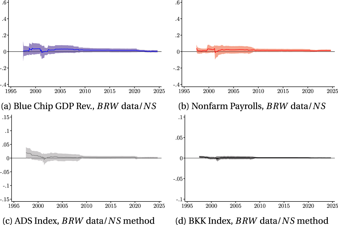
Predictability coefficients with 95 % confidence intervals. Real-Time Estimate of
B Appendix: Forecast Revision Specification
This section describes the data construction for the forecast revision specifications used to estimate monetary policy transmission.
This specification is estimated via OLS with Huber-White robust standard errors. The dependent variable is monthly GDP revisions for the year ahead. More specifically, for a given month we take the average of the revisions for the one-, two-, and three-quarter-ahead forecasts. The independent variable is the respective monetary policy shock being tested, excluding shocks occurring in either the first two (after December 2000) or three (before December 2000) business days of the month, as this is when the Blue Chip survey is still being collected. The sample is from January 1995 to September 2024.
The Independent Variable: Monetary Policy Shock
Each of the seven shock series studied are aggregated to a monthly frequency by summing values across the month. There are particular steps necessary to take before aggregation so that the aggregated monetary policy shocks of a month precede any Blue Chip output growth revision.
We drop meetings occurring before that month’s survey collection of Blue Chip is finished. Before December 2000, this was the fourth business day of the month but thereafter was the third business day of the month. This step has several sub-steps. Before December 1, 2000, we also drop any meetings within the first three business days of the month while after December 1, 2000 we drop any meetings within the first two business days of the month. Before December 1, 2000, this means that we drop monetary policy announcements that occur before the fourth day of the month or meetings that are either on the fifth or fourth day of the month and either a Monday, Tuesday, or Wednesday. After December 1, 2000 this means that we drop all meetings that occur before the third day of the month as well as meetings that are either on the third or fourth day of the month and on a Monday or a Tuesday. We then sum monetary policy shocks by month, excluding months during which there are no applicable FOMC meetings.
The Dependent Variable: GDP Forecast Revisions
The dependent variable is the median GDP forecast revision for the year ahead from the current month from the Blue Chip Economic Indicators. The Blue Chip releases GDP forecasts from the previous month within the first week of the current month. For example, the forecasts for October would be released within the first week of November.
Year-ahead forecast revisions are calculated as the average change in the one, two, and three-quarter-ahead median GDP forecasts for the current month. For example, the year-ahead output growth forecast revision for December 2007 is obtained by subtracting the GDP forecasts for 2008Q1, 2008Q2, and 2008Q3 from the November 2007 edition of the Blue Chip Economic Indicators from those from the December 2007 edition of the Blue Chip Economic Indicators (Appendix Figures (B.23)).
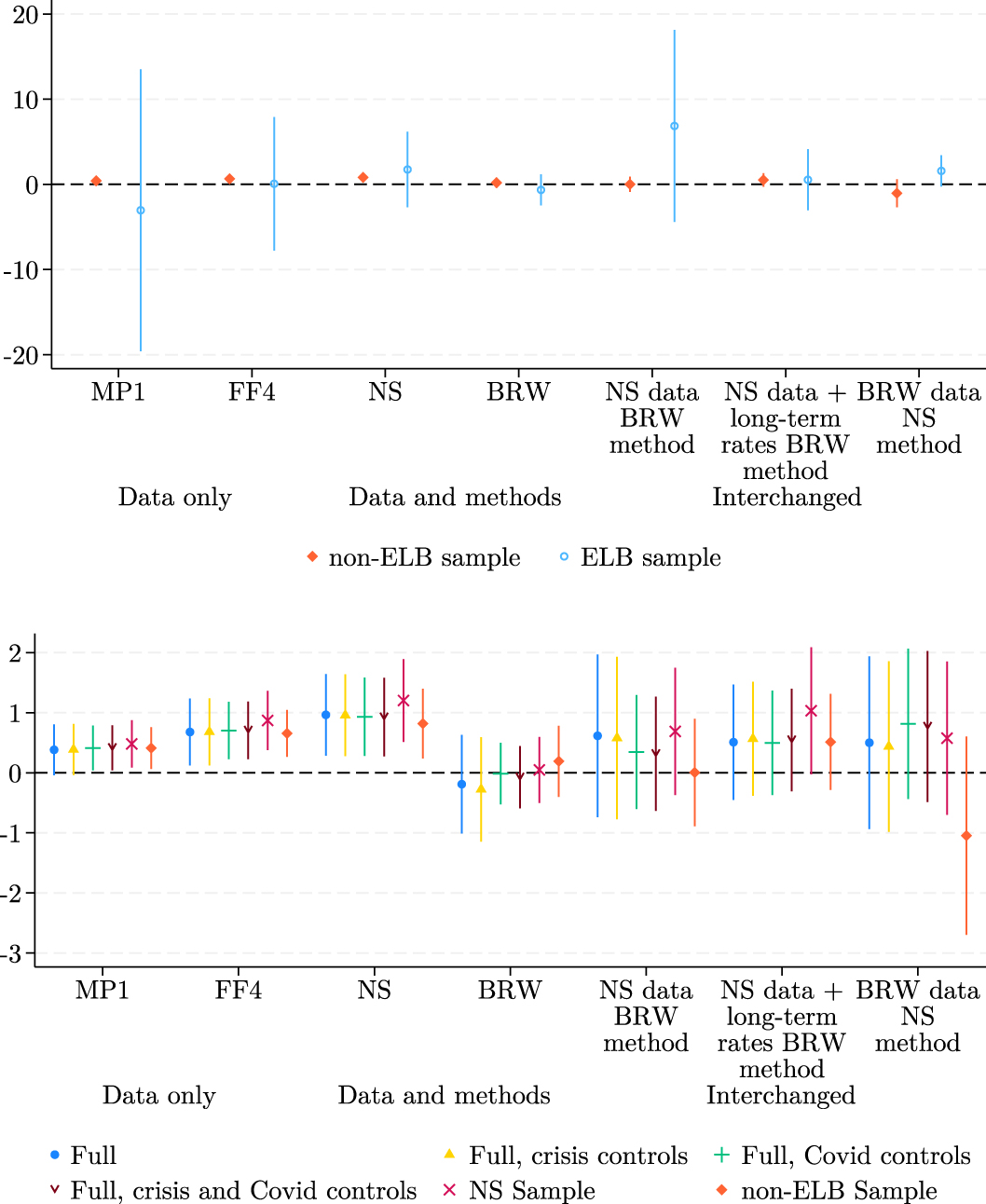
Forecast revision coefficients and 95 % confidence intervals. Estimates of
C Appendix: VAR
Using the Canova and Ferroni (2022) toolbox, we estimate the VAR specification of Bauer and Swanson (2022) for each of the seven monetary shock series studied in this paper. The monthly VAR has four economic variables: two-year zero-coupon Treasury yields, industrial production (IP), the consumer price index (CPI), and the Gilchrist and Zakrajšek (2012) excess bond premium, in that order. The two-year zero-coupon Treasury yield and Gilchrist and Zakrajšek (2012) excess bond premium are both divided by 100, and industrial production and CPI are transformed by taking logs. The two-year zero-coupon Treasury yield is aggregated from a daily to a monthly frequency by using the last observation for each month. Data series and their sources are described in more detail in Appendix D. Appendix Figure (C.24) plots the impulse response functions for the four economic variables to a 25 basis point NS shock.
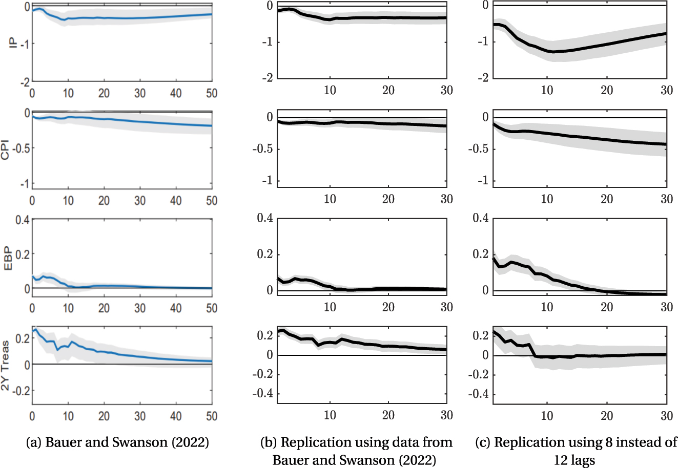
Impulse responses to a 25 basis point NS shock series, x-axis is months and y-axis is percentage points. Panel (a) is Figure (3) in Bauer and Swanson (2022). Estimates in panels (b) and (c) are from equation (13)
First, we reproduce Bauer and Swanson’s (2022) results with data from their website (https://www.michaeldbauer.com/files/FOMC_Bauer_Swanson.xlsx). Panel (C.24b) in the middle shows that our replication is a close match to their results shown in panel (C.24a) on the left. Differences in error bands arise due to slight variation in methodology. While we use the Bayesian VAR toolbox of Canova and Ferroni (2022), they use frequentist 90 % bootstrapped standard errors. However, these differences in error bands do not materially alter the implications of the estimates.
Second, we compare estimates from Bauer and Swanson (2022) to those from our construction of the NS shock series in a specification with 8 lags instead of 12. Bauer and Swanson’s (2022) version of the NS shock series is from February 1988 to December 2019 while ours is from January 1995 to September 2024. Following Swanson and Jayawickrema (2023), they obtain a longer sample by constructing the NS shock series using the first principal component of the {ED1/SF2, ED2/SF3, ED3/SF3, ED4/SF4} instrument set scaled by a 1 percentage point change in the ED4 rate instead of the {MP1, MP2, ED2/SF3, ED3/SF4, ED4/SF5} instrument set scaled by the daily change in the one-year zero-coupon Treasury.[16] With our relatively shorter sample for monetary shock series as an external instrument, we found that using 12 lags sacrifices too many degrees of freedom for error bands to be informative. We instead use 8 lags as a remedy and our results are shown in panel (C.24c). While there are quantitative differences in the magnitudes of the responses, such as impulse responses that are larger, the results are still quite similar to those of Bauer and Swanson (2022) shown on the left in panel (C.24a). Therefore, we proceed to implement our various monetary policy shocks as external instruments starting in 1995 in VARs with 8 lags. The increase in magnitudes of impulse responses as the sample shortens can be attributed to the prevalence of zero observations in the monetary shock series – after all, in most years there are four months without a monetary policy announcement. As the sample shortens, the zeros are more prominent and give rise to larger magnitudes.
D Appendix: Data
This section lists the source and description of each series used in this paper.
ADS Index is a daily business conditions index from Aruoba et al. (2009) and available for download from the Federal Reserve Bank of Philadelphia (https://www.philadelphiafed.org/surveys-and-data/real-time-data-research/ads).
Blue Chip GDP Forecast Revisions are the monthly forecast revision of the median GDP forecast. They are obtained from Haver Analytics’ Blue Chip Economic Indicators (http://www.haver.com/our_data.html).
BKK Index is a daily coincident index from Brave et al. (2019) that provides a summary statistic for the state of the economy. It is available for download from Indiana University Kelley School of Business (https://www.ibrc.indiana.edu/bbki/).
Constant Maturity Treasury Yields are daily market yields on U.S. Treasuries obtain via the H.15 Selected Interest Rate Release from the Federal Reserve Board.
Consumer Price Index is the seasonally adjusted monthly Consumer Price Index from the Bureau of Labor Statistics (FRED: CPIAUCSL_20210208).
Daily CPI The Billion Prices Project publicly available daily CPI can be obtained via Cavallo and Rigobon (2016) for July 2008 through August 2015 (https://dataverse.harvard.edu/dataset.xhtml?persistentId=doi%3A10.7910 %2FDVN%2F6RQCRS). This is series indexCPI for country == USA in spreadsheet pricestats_bpp_arg_usa.csv in folder all_files_in_csv_format.zip. Alternatively, the data are also available from the pricestats_bpp_ar_usa.dta file in the RAWDATA folder on the website https://www.openicpsr.org/openicpsr/project/113968/version/V1/view. The index is not seasonally adjusted constructed from webscraped prices of multichannel retailers that sell both online and offline.
Eurdollar Futures are available at an intraday tick frequency from 1995 to March 2023 via the CME Group Inc. DataMine (https://datamine.cmegroup.com/) at the Federal Reserve Board.
Excess Bond Premium is a monthly credit spread index from Gilchrist and Zakrajšek (2012) and is available from the Federal Reserve Board (https://www.federalreserve.gov/econres/notes/feds-notes/ebp_csv.csv.)
Federal Funds Futures are available at an intraday tick frequency from 1995 to present via the CME Group Inc. DataMine at the Federal Reserve Board (https://datamine.cmegroup.com/).
FOMC Announcement Dates and Times the dates of FOMC announcements for 1994–2024 are obtained directly from the Federal Reserve’s public website (https://www.federalreserve.gov/monetarypolicy/fomccalendars.htm). For selecting the exact times of the announcements, we first use the release time as printed on the FOMC’s public press release or otherwise on the Federal Reserve’s public website. This is possible for the meetings of 8/7/2007, 5/9/2010, and from 2016 to 2024. Whenever it is not possible to use release time from the Federal Reserve’s public website, we next take release times as recorded in the data of Gürkaynak et al. (2005), which covers meetings from 1995 to 2004. Finally, we consider the time of the first article on Bloomberg regarding the FOMC announcement, which mainly covers meetings from 2005 to 2015. We drop all notational meetings including August 27, 2000, October 4, 2019, March 11, 2008, and August 10, 2007. Following much of the literature, we drop the meetings after 9/11. We drop the March 15, 2020 unscheduled meeting as it occurred on a Sunday and it is difficult to source trades.
Industrial Production is the seasonally adjusted monthly Industrial Production Index from the Federal Reserve Board (ALFRED: INDPRO_20200616).
Nonfarm payrolls, all employees is the monthly total nonfarm payrolls release from the Bureau of Labor Statistic’s Current Employment Statistics Establishment Survey (FRED: PAYEMS).
SOFR Futures are used at an intraday tick frequency from January 2022 to September 2024 via the CME Group Inc. DataMine (https://datamine.cmegroup.com/) at the Federal Reserve Board.
Treasury Forward Rates are daily instantaneous forward rates (mnemonic: SVENFXX) obtained from the Federal Reserve Board (https://www.federalreserve.gov/data/yield-curve-tables/feds200628_1.html or as a csv file).
Zero-coupon Treasury Yields are continuously compounded zero-coupon daily yields (mnemonic: SVENYXX) obtained from the Federal Reserve Board (https://www.federalreserve.gov/data/yield-curve-tables/feds200628_1.html or as a csv file).
Yields of Treasury futures are the first expiring contracts and available per security via Bloomberg with the tickers TU1 COMB, FV1 COMB, TY1 COMB, US1 COMB.
References
Acosta, Miguel. 2023. “The Perceived Causes of Monetary Policy Surprises.” Working Paper.Search in Google Scholar
Acosta, Miguel, Connor M. Brennan, and Margaret M. Jacobson. 2024. “Constructing High-Frequency Monetary Policy Surprises from SOFR Futures.” Economics Letters 242 (September): 111873, https://doi.org/10.1016/j.econlet.2024.111873.Search in Google Scholar
Altavilla, Carlo, Luca Brugnolini, Refet S. Gürkaynak, Roberto Motto, and Giuseppe Ragusa. 2019. “Measuring Euro Area Monetary Policy.” Journal of Monetary Economics 108 (December): 162–79, https://doi.org/10.1016/j.jmoneco.2019.08.016.Search in Google Scholar
An, Phillip, Karlye Dilts Stedman, and Amaze Lusompa. 2025. “How High Does High Frequency Need to Be? A Comparison of Daily and Intraday Monetary Policy Surprises.” Working Paper.10.2139/ssrn.5319991Search in Google Scholar
Andrade, Philippe, and Filippo Ferroni. 2021. “Delphic and Odyssean Monetary Policy Shocks: Evidence from the Euro Area.” Journal of Monetary Economics 117 (January): 816–32, https://doi.org/10.1016/j.jmoneco.2020.06.002.Search in Google Scholar
Aruoba, Boragan and Thomas Drechsel. 2025. “Identifying Monetary Policy Shocks: A Natural Language Approach.” Working Paper.10.3386/w32417Search in Google Scholar
Aruoba, S. Boragan, Francis X. Diebold, and Chiara Scotti. 2009. “Real-Time Measurement of Business Conditions.” Journal of Business & Economic Statistics 27 (4): 417–27. https://doi.org/10.1198/jbes.2009.07205.Search in Google Scholar
Barakchian, S. Mahdi, and Christopher Crowe. 2013. “Monetary Policy Matters: Evidence from New Shocks Data.” Journal of Monetary Economics 60 (8): 950–66. https://doi.org/10.1016/j.jmoneco.2013.09.006.Search in Google Scholar
Bauer, Michael D., and Eric T. Swanson. 2022. “A Reassessment of Monetary Policy Surprises and High-Frequency Identification.” In NBER Macroeconomics Annual 2022, 37. Chicago and London: University of Chicago Press.10.3386/w29939Search in Google Scholar
Bauer, Michael D., and Eric T. Swanson. 2023. ““An Alternative Explanation for the” Fed Information Effect.” American Economic Review 113 (3): 664–700. https://doi.org/10.1257/aer.20201220.Search in Google Scholar
Boehm, Christoph E., and T. Niklas Kroner. 2025. “Monetary Policy without Moving Interest Rates: The Fed Non-yield Shock,” Working Paper.10.3386/w32636Search in Google Scholar
Braun, Robin, Silvia Miranda-Agrippino, and Tuli Saha. 2025. “Measuring Monetary Policy in the UK: The UK Monetary Policy Event-Study Database.” Journal of Monetary Economics (January): 103645, https://doi.org/10.1016/j.jmoneco.2024.103645.Search in Google Scholar
Brave, Scott A., Andrew Butters, and David Kelley. 2019. “A New “Big Data” Index of U.S. Economic Activity.” In Economic Perspectives. Federal Reserve Bank of Chicago.10.21033/ep-2019-1Search in Google Scholar
Bu, Chunya, John Rogers, and Wenbin Wu. 2021. “A Unified Measure of Fed Monetary Policy Shocks.” Journal of Monetary Economics 118 (March): 331–49, https://doi.org/10.1016/j.jmoneco.2020.11.002.Search in Google Scholar
Bundick, Brent, and A. Lee Smith. 2020. “The Dynamic Effect of Forward Guidance Shocks.” Review of Economics and Statistics 102 (5): 946–65. https://doi.org/10.1162/rest_a_00856.Search in Google Scholar
Caldara, Dario, and Edward Herbst. 2019. “Monetary Policy, Real Activity, and Credit Spreads: Evidence from Bayesian Proxy SVARs.” American Economic Journal: Macroeconomics 11 (1): 157–92. https://doi.org/10.1257/mac.20170294.Search in Google Scholar
Campbell, Jeffery R., Charles L. Evans, Jonas D. M. Fisher, and Alejandro Justiniano. 2012. “Macroeconomic Effects of Federal Reserve Forward Guidance.” Brookings Papers on Economic Activity (Spring): 1–54, https://doi.org/10.1353/eca.2012.0004.Search in Google Scholar
Canova, Fabio, and Filippo Ferroni. 2022. “A Hitchhiker’s Guide to Empirical Macro Models.” Working Paper.10.21033/wp-2021-15Search in Google Scholar
Carlstrom, Charles T., and Margaret M. Jacobson. 2013. Thresholds or Dates in Monetary Policy Communications. Federal Reserve Bank of Cleveland Economic Trends.Search in Google Scholar
Cavallo, Alberto, and Roberto Rigobon. 2016. “The Billion Prices Project: Using Online Data for Measurement and Research.” Journal of Economic Perspectives 31 (1).10.3386/w22111Search in Google Scholar
Christiano, Lawrence J., Martin Eichenbaum, and Charles Evans. 1996. “The Effects of Monetary Policy Shocks: Evidence from the Flow of Funds.” The Review of Economics and Statistics 78 (1): 16–34. https://doi.org/10.2307/2109845.Search in Google Scholar
Christiano, Lawrence J., Martin Eichenbaum, and Charles L. Evans. 2005. “Nominal Rigidities and the Dynamic Effects of a Shock to Monetary Policy.” Journal of Political Economy 113 (1): 1–45. https://doi.org/10.1086/426038.Search in Google Scholar
Cieslak, Anna, and Andreas Schrimpf. 2019. “Non-monetary News in Central Bank Communication.” Journal of International Economics 118 (May): 293–315, https://doi.org/10.1016/j.jinteco.2019.01.012.Search in Google Scholar
Ettmeier, Stephanie, and Alexander Kriwoluzky. 2019. “Same, but Different? Testing Monetary Policy Shock Measures.” Economics Letters 184 (November): 108640, https://doi.org/10.1016/j.econlet.2019.108640.Search in Google Scholar
Fama, Eugene F., and James D. MacBeth. 1973. “Risk, Return, and Equilibrium: Empirical Tests.” Journal of Political Economy 81 (3): 607–36. https://doi.org/10.1086/260061.Search in Google Scholar
Gertler, Mark, and Peter Karadi. 2015. “Monetary Policy Surprises, Credit Costs, and Economic Activity.” AEJ: Macroeconomics 7 (January): 44–76, https://doi.org/10.1257/mac.20130329.Search in Google Scholar
Gilchrist, Simon, and Egon Zakrajšek. 2012. “Credit Spreads and Business Cycle Fluctuations.” American Economic Review 102 (4): 1692–720. https://doi.org/10.1257/aer.102.4.1692.Search in Google Scholar
Gürkaynak, Refet S., Brian P. Sack, and Eric T. Swanson. 2005. “Do Actions Speak Louder Than Words? the Response of Asset Prices to Monetary Policy Actions and Statements.” International Journal of Central Banking 1 (May): 55–93.10.2139/ssrn.633281Search in Google Scholar
Gürkaynak, Refet S., Brian P. Sack, and Eric T. Swanson. 2007b. “Market-Based Measures of Monetary Policy Expectations.” Journal of Business & Economic Statistics 25 (2): 201–12.10.1198/073500106000000387Search in Google Scholar
Gürkaynak, Refet S., Brian Sack, and Jonathan H. Wright. 2007a. “The U.S. Treasury Yield Curve: 1961 to the Present.” Journal of Monetary Economics 54 (8): 2291–304.10.1016/j.jmoneco.2007.06.029Search in Google Scholar
Gürkaynak, Refet S., Burçin Kısacıkoğlu, and Sang Seok Lee. 2023. “Exchange Rate and Inflation under Weak Monetary Policy: Turkey Verifies Theory.” Economic Policy 38 (115): 519–60. https://doi.org/10.1093/epolic/eiad020.Search in Google Scholar
Hansen, Stephen, Michael McMahon, and Matthew Tong. 2019. “The Long-Run Information Effect of Central Bank Communication.” Journal of Monetary Economics 108 (December): 185–202, https://doi.org/10.1016/j.jmoneco.2019.09.002.Search in Google Scholar
Hanson, Samuel G., and Jeremy C. Stein. 2015. “Monetary Policy and Long-Term Real Rates.” Journal of Financial Economics 115 (March): 429–48, https://doi.org/10.1016/j.jfineco.2014.11.001.Search in Google Scholar
Jacobson, Margaret M., Christian Matthes, and Todd B. Walker. 2025. “Temporal Aggregation Bias and Monetary Policy Transmission,” Working Paper.Search in Google Scholar
Jarociński, Marek. 2024. “Estimating the Fed’s Unconventional Policy Shocks.” Journal of Monetary Economics 144 (May): 103548, https://doi.org/10.1016/j.jmoneco.2024.01.001.Search in Google Scholar
Jarociński, Marek, and Peter Karadi. 2020. “Deconstructing Monetary Policy Surprises: The Role of Information Shocks.” AEJ:Macroeconomics 12 (2). https://doi.org/10.1257/mac.20180090.Search in Google Scholar
Karnaukh, Nina, and Petra Vokata. 2022. “Growth Forecasts and News about Monetary Policy.” Journal of Financial Economics 146 (1): 55–70. https://doi.org/10.1016/j.jfineco.2022.07.001.Search in Google Scholar
Kuttner, Kenneth N. 2001. “Monetary Policy Surprises and Interest Rates: Evidence from the Fed Funds Futures Market.” Journal of Monetary Economics 47 (June): 523–44, https://doi.org/10.1016/s0304-3932(01)00055-1.Search in Google Scholar
Lewis, Daniel J. 2025. “Announcement-Specific Decompositions of Unconventional Monetary Policy Shocks and Their Effects.” The Review of Economics and Statistics 107 (4): 1086–103.10.1162/rest_a_01315Search in Google Scholar
McKay, Alisdair, and Christian K. Wolf. 2023. “What Can Time-Series Regressions Tell us about Policy Counterfactuals?” Econometrica 91 (5): 1695–725, https://doi.org/10.3982/ecta21045.Search in Google Scholar
Miranda-Agrippino, Silvia, and Hélène Rey. 2020. “The Global Financial Cycle after Lehman.” AEA Papers and Proceedings 110 (May): 523–8, https://doi.org/10.1257/pandp.20201096.Search in Google Scholar
Miranda-Agrippino, Silvia, and Giovanni Ricco. 2021. “The Transmission of Monetary Policy Shocks.” American Economic Journal: Macroeconomics 13 (3): 74–107. https://doi.org/10.1257/mac.20180124.Search in Google Scholar
Miranda-Agrippino, Silvia, and Giovanni Ricco. 2023. “Identification with External Instruments in Structural VARs.” Journal of Monetary Economics 135 (C): 1–19. https://doi.org/10.1016/j.jmoneco.2023.01.006.Search in Google Scholar
Nakamura, Emi, and Jón Steinsson. 2018. “High-Frequency Identification of Monetary Non-neutrality: The Information Effect.” Quarterly Journal of Economics 133 (3): 1283–330, https://doi.org/10.1093/qje/qjy004.Search in Google Scholar
Nunes, Ricardo, Ali Ozdagli, and Jenny Tang. 2023. “Interest Rate Surprises: A Tale of Two Shocks.” Discussion Papers 2320, Centre for Macroeconomics (CFM).10.2139/ssrn.4524624Search in Google Scholar
Paul, Pascal. 2020. “The Time-Varying Effect of Monetary Policy on Asset Prices.” The Review of Economics and Statistics 102 (4): 690–704. https://doi.org/10.1162/rest_a_00840.Search in Google Scholar
Piazzesi, Monika, and Eric T. Swanson. 2008. “Futures Prices as Risk-Adjusted Forecasts of Monetary Policy.” Journal of Monetary Economics 55 (4): 677–91. https://doi.org/10.1016/j.jmoneco.2008.04.003.Search in Google Scholar
Ramey, V. A. 2016. “Chapter 2 - Macroeconomic Shocks and Their Propagation.” In Handbook of Macroeconomics, 2, edited by John B. Taylor, and Harald Uhlig, 71–162. Amsterdam and Oxford: Elsevier.10.1016/bs.hesmac.2016.03.003Search in Google Scholar
Rigobon, Roberto. 2003. “Identification through Heteroskedasticity.” The Review of Economics and Statistics 85 (4): 777–92. https://doi.org/10.1162/003465303772815727.Search in Google Scholar
Romer, Christina D., and David H. Romer. 1989. “Does Monetary Policy Matter? A New Test in the Spirit of Friedman and Schwartz.” In NBER Macroeconomics Annual 1989, edited by Olivier J. Blanchard, and Stanley Fischer, 121–70. Cambridge, MA: MIT Press.10.1086/654103Search in Google Scholar
Romer, Christina D., and David H. Romer. 2004. “A New Measure of Monetary Shocks: Derivation and Implications.” American Economic Review 94 (4): 1055–84. https://doi.org/10.1257/0002828042002651.Search in Google Scholar
Rudebusch, Glenn D. 1998. “Do Measures of Monetary Policy in a Var Make Sense?” International Economic Review 39 (4): 907–31. https://doi.org/10.2307/2527344.Search in Google Scholar
Sastry, Karthik A. 2021. “Disagreement About Monetary Policy.” working paper.Search in Google Scholar
Sims, Christopher A. 1998. ““Comment on Glenn Rudebusch’s” Do Measures of Monetary Policy in a Var Make Sense?” International Economic Review 39 (4): 933–41. https://doi.org/10.2307/2527345.Search in Google Scholar
Stavrakeva, Vania, and Jenny Tang. 2024 Forthcoming. “The Dollar During the Great Recession: US Monetary Policy Signaling and the Flight to Safety.” Journal of Finance.10.2139/ssrn.4905627Search in Google Scholar
Stock, James, and Mark Watson. 2018. “Identification and Estimation of Dynamic Causal Effects in Macroeconomics Using External Instruments.” Economic Journal 128 (610): 917–48. https://doi.org/10.1111/ecoj.12593.Search in Google Scholar
Swanson, Eric T. 2021. “Measuring the Effects of Federal Reserve Forward Guidance and Asset Purchases on Financial Markets.” Journal of Monetary Economics 118 (March): 32–5, https://doi.org/10.1016/j.jmoneco.2020.09.003.Search in Google Scholar
Swanson, Eric T. 2023. “The Macroeconomic Effects of the Federal Reserve’s Conventional and Unconventional Monetary Policies,” Working Paper 31603.10.3386/w31603Search in Google Scholar
Swanson, Eric, and Vishuddhi Jayawickrema. 2023. “Speeches by the Fed Chair Are More Important Than FOMC Announcements: An Improved High-Frequency Measure of U.S. Monetary Policy Shocks.” Working Paper, UC Irvine.Search in Google Scholar
Swanson, Eric T., and John C. Williams. 2014. “Measuring the Effect of the Zero Lower Bound on Medium- and Longer-Term Interest Rates.” American Economic Review 104 (10): 3154–85. https://doi.org/10.1257/aer.104.10.3154.Search in Google Scholar
Vissing-Jorgensen, Annette, and Arvind Krishnamurthy. 2011. “The Effects of Quantitative Easing on Interest Rates: Channels and Implications for Policy.” Brookings Paper on Economic Activity 42 (2): 215–87, https://doi.org/10.1353/eca.2011.0019.Search in Google Scholar
Wieland, Johannes F., and Mu-Jeung Yang. 2020. “Financial Dampening.” Journal of Money, Credit and Banking 52 (1): 79–113. https://doi.org/10.1111/jmcb.12681.Search in Google Scholar
Zhu, Linyan. 2023. “Let the Market Speak: Using Interest Rates to Identify the Fed Information Effect.” Working Paper.10.2139/ssrn.4035869Search in Google Scholar
© 2025 Walter de Gruyter GmbH, Berlin/Boston
Articles in the same Issue
- Frontmatter
- Advances
- Real Wage Cyclicality and Monetary Policy
- Green Transition, Skills Heterogeneity, and Inequality
- Workforce Aging, Growth and Productivity
- Monetary Policy Shocks: Data or Methods?
- Contributions
- Monetary Policy and Labor Market Friction in a HANK Model
- Capital Market Liberalization and Bank Credit Decisions: A Quasi-Natural Experiment Based on the “Mainland-Hong Kong Stock Connect”
- Automation, Skill Premium, and Labor Share
- Business Cycles, Monetary Policy Stance, and Monetary Policy Transmission in Korea
- Forecasting Revisions to U.S. Jobs Report Data
- Loan Loss Provision, Unsecured-Collateralized Loan Choice and Macro-Stability in China
- Price Stickiness, Input–Output Linkages, and Monetary Policy Transmission in Korea
- Oil Price-Driven Inflation and the Channels of Pass-Through
- Firm Dynamics, Informality, and Monetary Policy