Reconstruction of Tesla micro-valve using topological sensitivity analysis

M. Abdelwahed; N. Chorfi; R. Malek

doi:10.1515/anona-2020-0014

Artikel Open Access

Reconstruction of Tesla micro-valve using topological sensitivity analysis

M. Abdelwahed , N. Chorfi und R. Malek

Veröffentlicht/Copyright: 16. Juni 2019

Veröffentlicht von

Veröffentlichen auch Sie bei De Gruyter Brill

Manuskript einreichen Informationen für Autor*innen Erkunden Sie dieses Fachgebiet

Aus der Zeitschrift Advances in Nonlinear Analysis Band 9 Heft 1

Abstract

In this paper, we deal with topology optimization attributed to the non stationary Navier-Stokes equations. We propose an approach where we analyze the sensitivity of a shape function relating to a perturbation of the flow domain. A numerical optimization algorithm based on topological gradient method is built and applied to the 2D Tesla micro valve reconstruction. Some numerical results confirm the efficiency of the proposed approach.

Keywords: Non-stationary Navier-Stokes equations; Tesla valve; Shape optimization; Topological sensitivity method

1 Introduction

Tesla valves are no-moving-part valves that utilize fluidic inertial forces to inhibit flow in the reverse direction. It was patented in 1920 by Nikola Tesla as a “Valvular conduit” [1] (see figure 1), and has since made the subject of various applications in micro-satellite [2], drug delivery [3], microbiology [4, 5] and hydrocephalus treatment in medicine [6, 7].

Fig. 1

A rotated scanning electron microscope photograph of a Tesla valve by Forster et al. [8]

The Tesla micro-valve performance is evaluated by the diodicity parameter (represents the ratio of the pressure drop in backward and forward direction) which evaluates the ability of allowing forward flow while inhibiting the reverse one,

Di=ΔpbackwardΔpforward.

Different works have focused on the optimal shape of the tesla micro-valve. However, the majority of works concerns stationary Partial Differential Equations (PDE). Forster et al. [8] proved the possibility of using Tesla valves in micro-fluidics and determined experimentally the diodicity for Reynolds number (Re) ≃ 180. Truong et al. in [9] derived numerically the optimum geometry of Tesla valve for 100 < Re < 600 with better diodicity than [8]. Bardell et al [10] analyzed the mechanism of the diodicity and proposed a Tesla valve optimal design for low Re. In the case when Re = 100, they finished with Di = 1.4. Gamboa et al. [11] optimized the shape of Tesla valve for application with piezoactuated plenums. The obtained fluid domain related to Re = 100 is characterized by a diodicity number Di = 1.1. In 2008, Pingen et al. [12] used the Lattice Bolzmann Method for the optimization of a micro Tesla valve without any information on diodicity. The used objective function was the pressure drop between inlet and outlet. After that in 2010, Lin et al. [13] used a topology optimization technique based on the power dissipation energy [14] of forward flow as objective function and the diodicity was built into the model as a constraint. For Re = 100, they found a new design of Tesla valve given Di = 1.2. Next in 2015, Lin et al. [15] solved the Tesla valve topology optimization using the approach of material distribution with inverse diodicity as objective function and fluid volume fraction as the constraint.

Until recently, there were no investigations dealing with the non-stationary case. We propose in this paper a new reconstruction method using the sensitivity analysis approach [16, 17, 18, 19] for a non stationary flow.

The principal results of this work concern both theoretical and numerical aspects associated with the Tesla micro-valve problem. The theoretical part is related to the analysis of the topological sensitivity for the non stationary Navier-Stokes equations. The numerical part concerns the 2D optimization of the Tesla micro-valve shape. The optimal shape is constructed by inserting obstacles in the considered initial domain. We build a simple and fast numerical reconstruction algorithm based on the topological gradient technique. The efficiency of the presented approach is confirmed by some numerical tests.

The paper is presented as following: Firstly we formulate the problem in section 2. Section 3 concerns the theoretical aspects. The numerical aspects are given in section 4. Finally section 5 includes Theorems proofs.

2 Problem formulation

Let Ω ⊂ ℝ^d, d = 2, 3 a bounded domain with regular boundary Γ = ∂Ω. We consider the blood as an incompressible viscous fluid flow described by the non stationary Navier-Stokes equations [20]. The velocity w and the pressure p satisfy the following system:

∂w∂t+∇w⋅w−νΔw+∇p=Gin Ω×]0,T[,divw=0in Ω×]0,T[,w=wdon Γ×]0,T[,w(.,0)=0in Ω, (1)

where ν is the kinematic viscosity coefficient, G is the gravitational force, T is the computational time and w_d is a given Dirichlet boundary data. Because of the divergence free condition on w, w_d must necessarily satisfy the compatibility condition,

∫Γwd(x,t).nds(x)=0,a.e. t∈]0,T[

where n is the unit outward normal vector along Γ.

Remark 2.1

Problem (1) has at least one solution (see [21](Ch.II, eq.(1.89)). If |w|_1,Ω < ν/k, with

k=223 meas(Ω)1/6if d=3,12 meas(Ω)1/2if d=2,

then problem (1) has a unique solution (see [17]).

The topological sensitivity method idea is to study the variation of a given shape function j relating to a perturbation in the fluid flow domain geometry.

In structural shape optimization case (respectively electromagnetism and fluid dynamics cases) a geometry perturbation means removing some material (respectively the insertion of an obstacle).

Let 𝓞_z,ε = z + ε𝓞, a small obstacle inserted in Ω characterized by its center z, its size ε and its shape 𝓞. 𝓞 is a bounded domain of ℝ^d containing the origin and ∂𝓞 (its boundary) is connected and piecewise 𝓒¹.

The shape function variation is written

j(Ω∖Oz,ε¯)−j(Ω)=ρ(ε)δj(z)+o(ρ(ε)),∀z∈Ω

where

ε ↦ ρ(ε), a positive scalar function going to zero with ε
z ↦ δj(z), called the topological gradient, describes the shape function variation when an obstacle is inserted in z. It plays the role of descent direction in the algorithm of optimization.

To our knowledge, the majority of works leading with topological sensitivity method concern the stationary case such as Stokes problem [16, 18], quasi-Stokes [19], stationary Navier Stokes problem [17]. We extend this method to the nonlinear unsteady Navier Stokes flow. To overcome the difficulty due to the non linear operator and its associated adjoint problem we extend the perturbed velocity by zero in the inclusion which permits to use the adjoint method in the whole domain. For the time dependent term we will use the fundamental solution of the non stationary Stokes operator and decompose the velocity variation.

We define the time dependent shape function as:

j(Ω∖Oz,ε¯)=∫0TJε(wε(.,t))dt, (2)

where J_ε in H¹(Ω ∖ 𝓞_z,ε)^d and w_ε is solution to

∂wε∂t+∇wε⋅wε−νΔwε+∇pε=Gin Ωz,ε×]0,T[,divwε=0in Ωz,ε×]0,T[,wε=wdon Γ×]0,T[,wε=0on ∂Oz,ε×]0,T[,wε(.,0)=0in Ωz,ε, (3)

with Ω_z,ε = Ω ∖ 𝓞_z,ε is the perturbed domain. Note that if ε = 0 (without obstacle), (w₀, p₀) verify (1) and Ω₀ = Ω.

In the following, we will derive a general mathematical analysis for J_ε satisfying the following assumption:

Assumption (𝓐)

∀ε ≥ 0, t ↦ J_ε(w_ε(., t)) ∈ L¹(0, T).
J₀ is differentiable in H¹(Ω) and we denote DJ₀(w) its derivative.
∃ρ : ℝ₊ ⟶ ℝ₊ and δ𝓙 ∈ ℝ such that ∀ε ≥ 0

∫0T[Jε(wε(.,t))−J0(w0(.,t))]dt=∫0TDJ0(w0(.,t))(wε(.,t)−w0(.,t))dt+ρ(ε)δJ+o(ρ(ε)).

3 Main results

We deal in this section with the non stationary Navier-Stokes topological sensitivity relating to the domain perturbation. We consider the shape functions verifying the assumption (𝓐).

3.1 Asymptotic behavior of the velocity variation

We first study the influence on the velocity v_ε = w_ε – w₀ of inserting a small obstacle O_z,ε in Ω. From (1) and (3), it is straightforward to show that (v_ε, p_{v_ε}) satisfy the system

∂vε∂t+∇vε⋅vε−νΔvε+∇vε⋅w0+∇w0⋅vε+∇pvε=0in Ωz,ε×]0,T[,divvε=0in Ωz,ε×]0,T[,vε=0on Γ×]0,T[,vε=−w0on ∂Oz,ε×]0,T[,vε(.,0)=0in Ωz,ε. (4)

We will distinguish in the following the 2D and 3D cases.

3.1.1 Three dimensional case

Theorem 3.1

There exists c > 0 independent of ε, such that

∥vε(x,t)−W(x,t)∥L2(0,T;H1(Ωz,ε))≤cε,

where W = (W¹, W², W³) ∈ H¹(Ω_z,ε)³ is defined by

Wj(x,t)=Uj(x−zε).w0(z,t),∀(x,t)∈R3∖O¯ε×]0,T[, (5)

with U^j is solution of (exterior Stokes problem)

−νΔUj+∇Pj=0inR3∖O¯,divUj=0inR3∖O¯,Uj⟶0at∞,Uj=−ejon∂O, (6)

with {e_j}_j=1,2,3 is the ℝ³ canonical basis.

We show by using a single layer potential (see [22]) that

Uj(y)=∫∂OE(y−x)ηj(x)ds(x),Pj(y)=∫∂OΠ(y−x)ηj(x)ds(x),∀y∈R3∖O¯.

where

E(y)=18πνr(I+ererT),Π(y)=y4πr3∀y∈R3.

with r = ∥y∥, e_r = yr,erT is the transpose of e_r and η_j ∈ H^–1/2(∂𝓞)³ is a solution of the boundary integral equation

∫∂OE(y−x)ηj(x)ds(x)=−ej,∀y∈∂O. (7)

Using Theorem 3.1 we obtain the following corollary.

Corollary 3.2

We have

vε(x,t)=W(x,t)+O(ε),x∈Ωz,ε,t∈]0,T[.

3.1.2 Two dimensional case

Theorem 3.3

There exists c > 0 independent on ε, verifying

∥vε(x,t)−1log⁡(ε)W(x,t)∥L2(0,T;H1(Ωz,ε))≤−clog⁡(ε),

where

W(x,t)=4πν∑j=12[Ej(x−z)w0(z,t)]ej,∀(x,t)∈Ωz,ε×]0,T[, (8)

with E^j(y) = E(y)e_j, 1 ≤ j ≤ 2, {e_j}_j=1,2 is the ℝ² canonical basis and

E(y)=14πν(−log⁡(r)I+ererT),Π(y)=y2πr2,∀y∈R2,

represents the fundamental solution of the Stokes System in ℝ² with r = ∥y∥ and e_r = yr .

Using Theorem 3.3 it follows the velocity estimation in the perturbed fluid flow domain.

Corollary 3.4

We have

vε(x,t)=W(x,t)+O(−1log⁡(ε)),x∈Ωz,ε,t>0.

3.2 Asymptotic behavior of the shape function

The topological sensitivity analysis for the non stationary Navier-Stokes operator in three and two dimensional cases is given in this section. The presented results are satisfied by all shape functions j defined by (2) and J_ε verifies the Assumption (𝓐).

3.2.1 Three dimensional case

Theorem 3.5

If J_ε satisfies the Assumption (𝓐) with ρ(ε) = ε, then j defined by (2) verifies

j(Ω∖Oz,ε¯)=j(Ω)+ε[∫0Tw0(z,t).MOu0(z,t)dt+δJ]+o(ε),

where

the matrix 𝓜_𝓞 is given by

MOij=∫∂Oηji(y)ds(y),1≤i,j≤3.
u₀ is the solution to the adjoint problem

−∂u0∂t−∇u0⋅w0+∇w0T⋅u0−νΔu0+∇pu0=−DJ0(w0)inΩ×]0,T[,divu0=0inΩ×]0,T[,u0=0onΓ×]0,T[,u0(.,T)=0inΩ. (9)

Corollary 3.6

If 𝓞 = B(0, 1) (the unit ball), η_j(y) = 3ν2ej,∀y∈∂O and

j(Ω∖Oz,ε¯)=j(Ω)+ε[∫0T6πνw0(z,t).u0(z,t)dt+δJ]+o(ε).

3.2.2 Two dimensional case

Theorem 3.7

If J_ε satisfies the Assumption (𝓐) then j defined by (2) verifies

j(Ω∖Oz,ε¯)=j(Ω)+−1log⁡(ε)[4πν∫0Tw0(z,t)u0(z,t)dt+δJ]+o(−1log⁡(ε)),

where u₀ is the adjoint state solution to the problem (9).

The proofs of Theorems 3.1, 3.3, 3.5 and 3.7 are relegated to section 5. The variation δ𝓙 depends on the shape functions expressions. Some useful examples in numerical applications will be presented in section 3.3.

3.3 Shape function examples

3.3.1 First example

We define the shape function

j(Ω∖Oz,ε¯)=∫0T∫Ωz,εwε−Wd(.,t)2dxdt

where 𝓦_d ∈ L¹(0, T; H¹(Ω)) is a datum representing a desired fluid flow state.

This example concerns the L²-norm shape function that has been used in geometric control problems like the optimization of location of some obstacle in a tank to approximate an object flow 𝓦_d (see [16]).

Proposition 3.8

The function

Jε(w)=∫Ωz,εw−Wd(.,t)2dx,∀w∈H1(Ωz,ε),

satisfies the assumption (𝓐) with

DJ0(w0(.,t))v=2∫Ω(w0(.,t)−Wd(.,t))vdx,∀v∈H1(Ω),δJ(z)=0,∀z∈Ω.

3.3.2 Second example

We define the shape function which corresponds to the dissipation energy minimization

j(Ω∖Oz,ε¯)=∫0T∫Ωz,ε∇wε−∇Wd(.,t)2dxdt,

where 𝓦_d ∈ L¹(0, T; H²(Ω)) is a given datum. It was used in several optimization problems such as minimum drag problem [23], pipe bend design [10?], cavity example [24], reconstruction of Tesla valve [13].

Proposition 3.9

The function

Jε(w)=∫Ωz,εν∇w−∇Wd(.,t)2dx,∀w∈H1(Ωz,ε),

satisfies the assumption (𝓐) with

DJ0(w0(.,t))v=2ν∫Ω(∇w0(.,t)−∇Wd(.,t))∇vdx,∀v∈H1(Ω),δJ(z)=4πν∫0T|w0(z,t)|2dt,∀z∈Ωif d=2,−∫0T(∫∂Oη(y)ds(y)).w0(z,t)dt,∀z∈Ωif d=3.

4 Numerical results

In this section, we deal with some numerical applications to validate the obtained theoretical results given in section 3.

4.1 Validation of the asymptotic expansion

To establish the numerical validation of Theorem 3.7, we consider the variation relating to ε of

Δz(ε)=j(Ω∖Oz,ε¯)−j(Ω)+1log⁡(ε)δj(z),

where

δj(z)=4πν∫0Tw0(z,t)u0(z,t)dt+δJ. (10)

We expect to prove numerically that Δ_z(ε) satisfies the previously derived theoretical estimate Δ_z(ε) = o(−1log⁡(ε)).

To this aim, we consider the following data:

Ω = ]0, 1[×]0, 1[ is a square domain.
The locations zεi = z_i + εB(0, 1) of the considered obstacles are arbitrary chosen (see Table 1).

Table 1

Location of obstacles

obstacle zεi zε1 zε2 zε3 zε4

location z_i z₁ = (0.2, 0.8) z₂ = (0.8, 0.2) z₃ = (0.5, 0.5) z₄ = (0.7, 0.7)
The shape function j is defined by the semi-norm

j(Ωz,ε)=∫0T∫Ωz,ε⏐∇wε−∇Wd⏐2dxdt, (11)

where 𝓦_d is a given velocity state.

In this case, the function Δ_{z_i}(ε) is defined by (see Theorem 3.7 and Proposition 3.9):

Δzi(ε)=j(Ω∖Oεi¯)−j(Ω)+4πνlog⁡(ε)(∫0Tw0(zi,t)u0(zi,t)dt+∫0T|w0(zi,t)|2dt).

The validation algorithm uses the following steps:

The validation algorithm:

Step 1:
1. compute the solution w₀ and the associated adjoint state u₀ in the domain Ω.
2. determine j(Ω) defined by (11).
Step 2: For each obstacle zεi = z_i + εB(0, 1), i = 1, …, 4:
1. determine the variation δj(z_i) given in (10),
2. choose ε0i = max {ε > 0, such that z_i + ε0i B(0, 1) ⊂ Ω},
3. compute an approximation of the function ε↦j(Ω∖Oεi¯),ε∈]0,ε0i].
Step 3: Deduce numerically the function ε↦log⁡(|Δzi(ε)|),ε∈]0,ε0i].

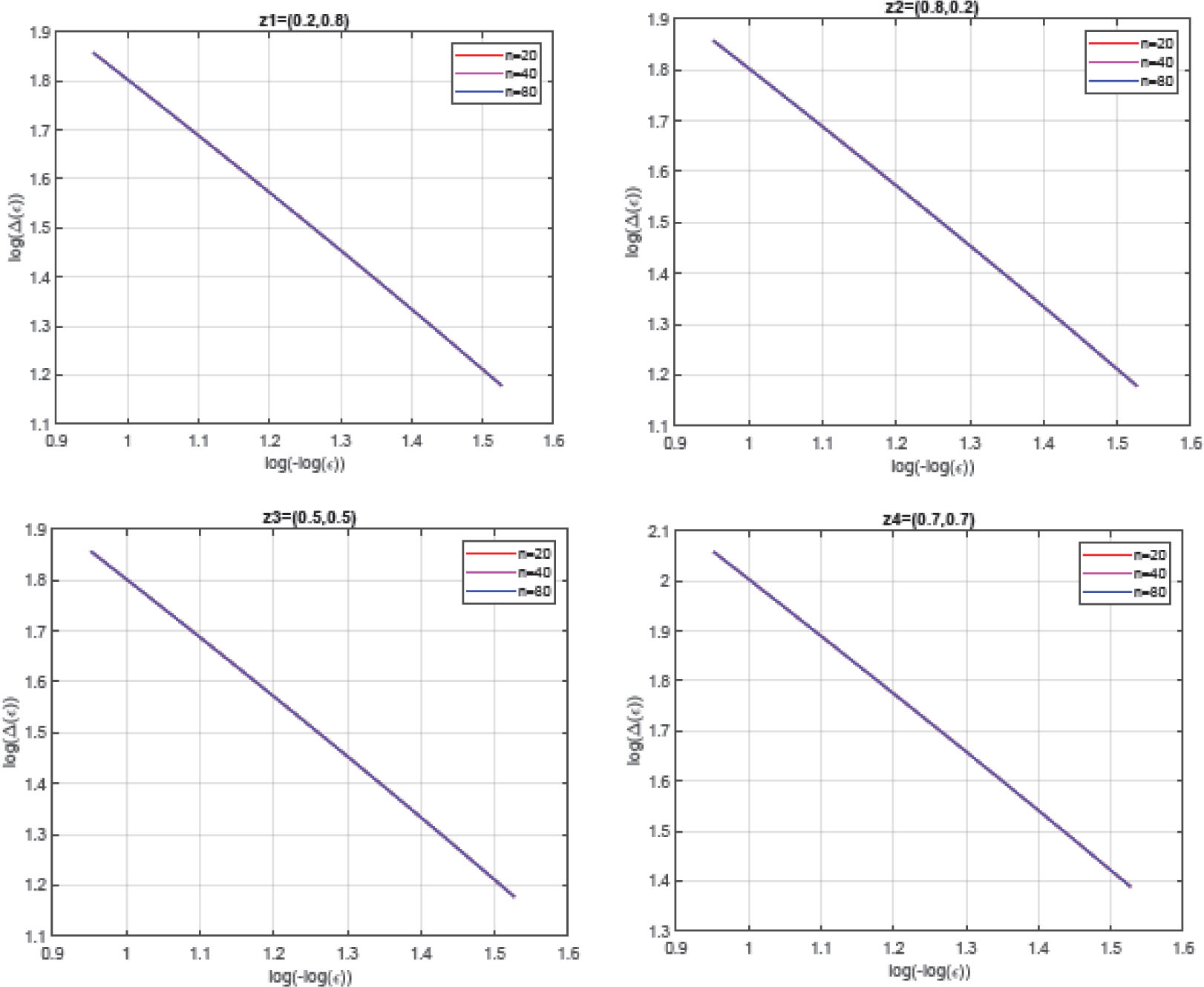
For each considered obstacle Oεi=zi+εB(0,1), we plot in Figure 2 the variation of log(|Δ_{z_i}(ε)|) relating to log(– log(ε)).

Fig. 2

Variation of log(|Δ_{z_i}(ε)|) relating to log(–log(ε)).

We define β_i to describe the behavior of ε ↦ Δ_{z_i}(ε) relating to –log(ε), i.e.

|Δzi(ε)|=O−log⁡(ε)βi.

It corresponds to the slope of the line approximating the variation ε ↦ log(|Δ_{z_i}(ε)|) relating to log(–log (ε)) for each obstacle zεi , i = 1, .., 4.

From the plotted curves in Figure 2, one deduce the slopes β_i, i = 1, …, 4 in table 2.

Table 2

The obtained slopes β_i of the lines associated with the obstacles Oεi , i = 1, ..., 4.

The considered obstacles Oεi	Oε1	Oε2	Oε3	Oε4
The obtained slopes β_i	–1.18	–1.187	–1.217	–1.163

We deduce that the numerical results confirm the behavior predicted by the theoretical estimate

Δzi(ε)=o(−1log⁡(ε)).

4.2 The Tesla micro-valve application

The hydrocephalus treatment is a very important application in medicine. The problem is to optimize numerically the design of the 2D Tesla micro-valve at Re = 100. To solve this problem we consider the objective function as the forward energy dissipation and the diodicity as a constraint. The optimal domain is constructed through the insertion of some obstacles in the initial one. The problem leads to optimize the location of obstacles.

4.2.1 Shape optimization problem

We define Ω as the pentagon [15] having one inclined inlet Γ_in and one horizontal outlet Γ_out (see Figure 3).

Fig. 3

Considered pentagon design domain

The aim is to find the fluid flow optimal domain Ω^∗ which minimizes the dissipated energy by the forward fluid flow and reproducing the original Tesla valve design given in Figure 1. This can be formulated:

Find Ω∗ solution to minΩ⊂Dadj(Ω), (12)

where

Dad={D⊂Ω such that Γin⊂Γ∩∂D,Γout⊂Γ∩∂D and |D|≤Vdesired},

with |.| and V_desired represents respectively the Lebesgue measure and the target volume.

We recall that the performance of the Tesla valve is measured by diodicity Di which is known as the ratio of the pressure drop in backward direction to that in forward direction, which is equivalent to the ratio of dissipation of reverse and forward flows [15]:

Di=Φ(wr)Φ(wf) with Φ(w)=∫Ω[ν2∑i,j(∂wi∂xj+∂wj∂xi)2],

with (w_f, p_f) and (w_r, p_r) are respectively the solution to the Navier Stokes system in the forward and the reverse flows. Then, diodicity can be maximized by minimizing forward dissipation while maximizing reverse dissipation. That is why our optimization problem is defined with the diodicity Di as a constraint; Di > 1.

Using the above definitions, the optimization problem [15] for reconstructing Tesla valve can be expressed as

Objective: power dissipation of forward flow

j(Ω)=Φ(wf)=ν∫0T∫Ω|∇wf|2dxdt,
Constraints
1. Volume fraction |V_desired| < 0.8 |V₀|.
2. Diodicity Di ≥ c > 1.
3. Navier Stokes equations for forward and backward directions.

We use the obtained theoretical results in 3.2.2 to solve (12).

4.2.2 The topology optimization process

To obtain the optimal domain, an iterative process is applied to construct a sequence of geometries (Ω_k)_k≥0 with Ω₀ = Ω and Ω_k+1 = Ω_k ∖ 𝓞_k where 𝓞_k is an obstacle inserted in Ω_k. To define the obstacle location and size, we find the function δj_k defined by (see Theorem 3.7)

δjk(z)=4πν[∫0T(wk(z,t)uk(z,t)+wk(z,t)2)dt],∀z∈Ωk, (13)

where

w_k represents the velocity, solution to the Navier-Stokes problem in Ω_k

∂wk∂t+∇wk⋅wk−νΔwk+∇pk=Gin Ωk×]0,T[,divwk=0in Ωk×]0,T[,wk=wdon Γ×]0,T[,wk=0on Σk×]0,T[,wk(.,0)=w0in Ωk. (14)
u_k is the adjoint state, solution to

−∂uk∂t−∇uk⋅wk−1+∇wk−1T⋅uk−νΔuk+∇qk=−DJ0(wk−1)in Ωk×]0,T[,divuk=0in Ωk×]0,T[,uk=0on Γ×]0,T[,uk=0on Σk×]0,T[,uk(.,T)=0in Ωk, (15)

where Σk=∂(∪l=0kOl) is the obstacle boundary inserted during the previous iterations. The optimization steps are summarized as:

The Algorithm:

Initialization: Set Ω₀ = Ω, and k = 0
Repeat until |Ω_k| ≤ V_desired:
1. The topological sensitivity function:
  1. compute w_k, solution to the non stationary Stokes problem (14) in Ω_k,
  2. compute v_k, solution to the associated adjoint problem (15) in Ω_k,
  3. compute the term δ𝓙_k and deduce the function δj_k(z), ∀z ∈ Ω_k.
2. The obstacle to be inserted:
  1. determine ρk⋆∈[0,1] such that j(Ωk∖Oρk⋆k¯)≤j(Ωk∖Oρk¯),∀ρ∈[0,1],
  2. set Ok={x∈Ωk;δjk(x)≤ρk⋆δmink}, where δmink=min(δjk(z)).
3. The new domain:
  1. set Ω_k+1 = Ω_k ∖ 𝓞_k,
4. k ⟵ k + 1 and go to (2).

The stopping criteria is defined by the natural optimality condition

δjk(x)≥0,∀x∈Ωk.

This algorithm is like a descent method where δj^k represents the descent direction and |𝓞_k| = |Ω_k ∖ Ω_k+1| the step length. The parameter ρk⋆ is chosen to allow ρ⟼j(Ωk∖Oρk¯) to decrease as much as possible. The computation of ρk⋆ in (b) can be viewed as line search step.

The numerical discretization of problems (14) and (15) is done by P1-bubble/P1 finite element method [25]. The computation of the approximated solutions is achieved by the Uzawa’s algorithm. The function δj^k is computed piecewise constant over elements.

Next, we will apply the proposed algorithm to reconstruct Tesla micro valve.

4.2.3 Reproducing the Tesla micro valve

We illustrate in this section the strengths of topology optimization method, namely the ability to find optimal design using only information on boundary conditions and constraints without the need of initial design.

The considered design domain is the pentagon domain (see Figure 3). This problem example has already been studied by S. Lin and al. in [15] in the steady state regime using projection method.

For the forward direction, the inlet boundary velocity has a parabolic behavior (Re = 100 relating to the inlet dimension). At the outlet boundary, the pressure is taken constant and no-slip condition is considered on the walls. For the backward flow direction, we reverse these boundary conditions. Besides, we prescribe solid regions close to the inlets/outlets to minimize the boundary effect on the final design solution.

We illustrate the geometries obtained during the optimization process in Figure 4. The optimal domain is obtained after four iterations. It is nearly identical to literature [1, 15] (see Figure 5).

Fig. 4

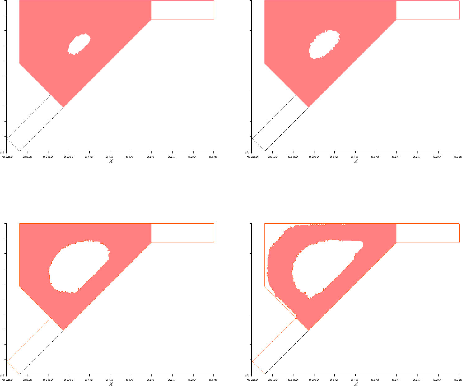
Geometries obtained during the optimization process

Fig. 5

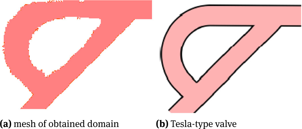
mesh of obtained design (left) and reference Tesla valve (right)

4.2.4 Discussion

In the previous Figure, thanks to the topological gradient, we deduce an easy reconstruction of tesla valve. Now, we normalize the obtained tesla valve behavior by plotting the obtained forward and reverse flows respectively in figures 6(a) and 6(b). It is clear that the velocity field is strongly different for the two cases.

Fig. 6

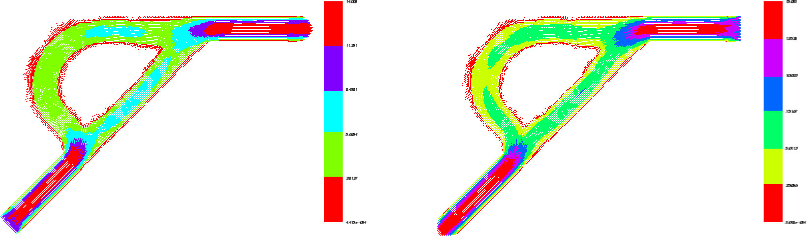
Forward and backward flow velocity field

To study the obtained tesla valve performance, we calculate the diodicity. Using the energy view point expression of diodicity, the experimentally derived value is 1.137. In bibliography [26], the diodicity is well predicted using

Di≅1+4.78∗10−5∗(N0.16Re1.72)

with N is the number of tesla valves and Re is the Reynolds number. Based on this expression, we found Di ≅ 1.1316 which ensures an agreement between the obtained diodicity and the experimental one.

5 Mathematical analysis

This section deals with the proofs of Theorems 3.1, 3.3, 3.5 and 3.7.

5.1 Proof of Theorem 3.1

Let Q be the pressure associated with the velocity W:

Q(x,t)=1εP(x−zε).w0(z,t)=1ε∑j=13Pj(x−zε)w0j(z,t), (16)

where P^j is the pressure associated with the velocity U^j solution to (6). Setting the variation

zε=vε−W and pzε=pvε−Q. (17)

From (4) and (6), we can verify that (z_ε, p_{z_ε}) is solution to

∂zε∂t−νΔzε+∇zε⋅(w0+W)+∇(w0+W)⋅zε+∇zε⋅zε+∇pzε=−∂W∂t−∇w0⋅W−∇W⋅w0−∇W⋅Win Ωz,ε×]0,T[,divzε=0in Ωz,ε×]0,T[,zε=−Won Γ×]0,T[,zε=−w0(x,t)+w0(z,t)on ∂Oε×]0,T[,zε(.,0)=0in Ωz,ε. (18)

The last boundary condition follows due to the fact that U^j = –e_j on ∂𝓞.

Moreover, since |w₀|_{L²(0,T;H¹(Ω))} < ν/k, then ε sufficiently small,

|w0+W|L2(0,T;H1(Ωz,ε))≤α<ν/k.

Let R > 0 such that 𝓞_z,ε ⊂ B(z, R) and B(z, R) ⊂ Ω. Using the trace theorem, we obtain

‖zε‖L2(0,T;H1(Ωz,ε))≤c(‖∂W∂t‖L2(0,T;L2(Ωz,ε))+‖W‖L2(0,T;H1(ΩR))+‖w0(x,t)−w0(z,t)‖L2(0,T;L2(Ωz,ε))+‖∇w0⋅W+∇W⋅w0+∇W⋅W‖L2(0,T;H−1(Ωz,ε))), (19)

where Ω_R = Ω ∖ B(z, R).

Using (5) and the variable change x = z + εy, we obtain

‖∂W∂t‖L2(0,T;L2(Ωz,ε))=‖∂w0∂t(z,.)‖L2(0,T)‖U(x−zε)‖L2(Ωz,ε)=ε3/2‖∂w0∂t(z,.)‖L2(0,T)‖U‖L2((Ωz,ε)/ε).

By the same way, we have

‖W‖L2(0,T;H1(ΩR))≤‖w0(z,.)‖L2(0,T)(‖U(x−zε)‖L2(ΩR)+‖∇xU(x−zε)‖L2(ΩR)),≤‖w0(z,.)‖L2(0,T)(ε3/2‖U‖L2((ΩR)/ε)+ε1/2‖∇yU‖L2(ΩR)/ε)).

Using [19] (see also [27]), the velocity field U^j, solution to the exterior Stokes problem, satisfies the estimate

‖Uj‖L2((ΩR)/ε)≤cε−1/2 and ‖∇yUj‖L2(ΩR)/ε)≤cε1/2.

Then, using the smoothness of w₀ and the previous estimates, one can deduce

‖∂W∂t‖L2(0,T;L2(Ωz,ε))≤cε and ‖W‖L2(0,T;H1(ΩR))≤cε. (20)

For the third term in (19). Expanding w₀(x, t) = w₀(z, t) + ε ∇ w₀(ξ_y, t)y with ξ_y ∈ 𝓞_z,ε and using the fact that ∇ w₀ is uniformly bounded, it follows that

‖w0(x,t)−w0(z,t)‖L2(0,T;L2(Ωz,ε))≤cε. (21)

We now examine the last term in (19). Since w₀ ∈ L^∞(Ω),

‖∇w0⋅W+∇W⋅w0+∇W⋅W‖L2(0,T;H−1(Ωz,ε))≤c(‖W‖L2(0,T;H−1(Ωz,ε))+‖∇W‖L2(0,T;H−1(Ωz,ε))+‖∇W⋅W‖L2(0,T;H−1(Ωz,ε))),≤c(‖W‖L2(0,T;L2(Ωz,ε))+|W|L2(0,T;H1(Ωz,ε))‖W‖L2(0,T;H1(Ωz,ε))),

according to Lemma 4.2 in [17].

In addition, by Lemma 4.5 in [17], the variable change and the continuity of w₀, we can deduce

‖W‖L2(0,T;L2(Ωz,ε))≤cε,|W|L2(0,T;H1(Ωz,ε))≤cε1/2 (22)

and then

‖∇w0⋅W+∇W⋅w0+∇W⋅W‖L2(0,T;H−1(Ωz,ε))≤cε. (23)

Finally, combining (20), (21) and (23) we deduce that

‖zε‖L2(0,T;H1(Ωz,ε))≤cε.

5.2 Proof of Theorem 3.3

Let Q be the pressure associated with the velocity W:

Q(x,t)=4πνΠ(x−z).w0(z,t)=4πν∑j=12Πj(x−z)w0j(z,t),

where Π^j is the pressure associated with the velocity E^j.

Setting

zε=vε−1log⁡(ε)W and sε=pvε−1log⁡(ε)Q. (24)

From (1) and (3), we obtain that (z_ε, s_ε) is solution to

∂zε∂t−νΔzε+∇zε⋅(w0+1log⁡(ε)W)+∇(w0+1log⁡(ε)W)⋅zε+∇zε⋅zε+∇sε=−1log⁡(ε)[∂W∂t−∇w0⋅W−∇W⋅w0−1log⁡(ε)∇W⋅W]in Ωz,ε×]0,T[,divzε=0in Ωz,ε×]0,T[,zε=−1log⁡(ε)Won Γ×]0,T[,zε=−w0(x,t)−4πνlog⁡(ε)E(x−z)w0(z,t)on ∂Oz,ε×]0,T[. (25)

Using the relation E((x−z)/ε)=E(x−z)+log⁡(ε)4πνI, the last boundary condition can be rewritten as

zε=−w0(x,t)+w0(z,t)−4πνlog⁡(ε)E((x−z)/ε)w0(z,t) on ∂Oz,ε×]0,T[.

Then, by an energy inequality [28], it follows

‖zε‖L2(0,T;H1(Ωz,ε))≤−clog⁡(ε)[‖∂W∂t‖L2(0,T;L2(Ωz,ε))+‖W‖L2(0,T;H1/2(Γ))+log⁡(ε)‖w0(z+εy,t)−w0(z,t)‖L2(0,T;H1/2(∂Oz,ε))+4πν‖E((x−z)/ε)w0(z,t)‖L2(0,T;H1/2(∂Oz,ε))+‖∇w0⋅W+∇W⋅w0+1log⁡(ε)∇W⋅W‖L2(0,T;L2(Ωz,ε))]. (26)

We estimate in the following each term in (26) separately.

We remark that:

Since 𝓞 is an open domain containing the origin, ∃r > 0 such that B(0, r) ⊂ 𝓞.
Ω is a bounded domain in such a way that ∃R > 0 such that Ω ⊂ B(z, R), ∀z ∈ Ω.
We have Ω_z,ε – z = {x – z, x ∈ Ω_z,ε} ⊂ C(0, rε, R) = {y ∈ ℝ²; rε < |y| < R}.

From the fact that C(0, rε, R) ⊂ ℝ² ∖ {0}, it follows that the function ψ : y ↦ log(|y|) is smooth in C(0, rε, R) and we have ∥ψ∥_0,C(0,rε,R) ≤ c. Then, using the cylindrical coordinate system, one can prove that ∃c > 0, independent of ε, such that

E(x−z)L2(0,T;L2(Ωz,ε))≤‖E(y)‖C(0,rε,R)≤c, (27)

∇E(x−z)L2(0,T;L2(Ωz,ε)≤c−log⁡(ε). (28)

Estimate of the first term in (26): Using that w₀ ∈ H¹(0, T; H¹(Ω)), we obtain

‖∂W∂t‖L2(0,T;L2(Ωz,ε))=4πν‖∂w0∂t(z,t)‖L2(0,T)‖E(x−z)‖L2(Ωz,ε)=O(1).
Estimate of the last term of (26):

Since w₀ and ∇ w₀ belong to L^∞(Ω), we have

‖∇w0⋅W+∇W⋅w0+1log⁡(ε)∇W⋅W‖L2(0,T;L2(Ωz,ε))≤c(‖W‖L2(0,T;L2(Ωz,ε))+‖∇W‖L2(0,T;L2(Ωz,ε))+1log⁡(ε)‖∇W‖L2(0,T;L2(Ωz,ε))‖W‖L2(0,T;L2(Ωz,ε))).

Using the definition of W, we can deduce the following estimates

‖W‖L2(0,T;L2(Ωz,ε))≤c,‖∇W‖L2(0,T;L2(Ωz,ε))≤c−log⁡(ε). (29)

Yet, we have

‖∇w0⋅W+∇W⋅w0+1log⁡(ε)∇W⋅W‖L2(0,T;L2(Ωz,ε))≤c−log⁡(ε). (30)
Estimate of boundary condition imposed on Γ:

Let R͠ > 0 such that 𝓞_z,ε ⊂ B(z, R͠) and B(z, R͠) ⊂ Ω. Since z ∉ Ω_R͠ = Ω ∖ B(z, R͠), the function x ↦ E(x – z) belongs to 𝓒¹(Ω_R͠). By the trace theorem, we have

‖W‖L2(0,T;H1/2(Γ)=4πν‖w0(z,t)‖L2(0,T)‖E(x−z)‖H1/2(Γ)≤4πν‖w0(z,t)‖L2(0,T)[‖E(x−z)‖L2(ΩR)+‖∇E(x−z)‖L2(ΩR)].

Therefore, ∥W∥_{L²(0,T;H^1/2(Γ)} is uniformly bounded with respect to ε.
Estimate of boundary condition imposed on ∂𝓞_z,ε:

Using the theorem of trace and the smoothness of w₀ in 𝓞_z,ε×]0, T[, one can obtain

‖w0(x,t)−w0(z,t)‖L2(0,T;H1/2(∂Oz,ε))≤cε.

Then, the first boundary term on ∂𝓞_z,ε satisfies

log⁡(ε)‖w0(x,t)−w0(z,t)‖L2(0,T;H1/2(∂Oz,ε))=o−1log⁡(ε).

To estimate the last boundary term, we use that 𝓞 contains the origin.

Setting 𝓞_r = 𝓞∖B(0, r) and 𝓞_{r, ε} = z + ε𝓞_r. Using the theorem of trace and the variable change x = z + εy, we obtain

‖E((x−z)/ε)w0(z,t)‖L2(0,T;H1/2(∂Oz,ε)) ≤‖w0(z,t)‖L2(0,T)(‖E((x−z)/ε)‖L2(Or,ε)+‖∇xE((x−z)/ε)‖L2(Or,ε)) ≤‖w0(z,t)‖L2(0,T)(ε‖E(y)‖L2(Or)+ε1/2‖∇yE(y)‖L2(Or)).

From the fact that y ↦ E(y) is sufficiently smooth in 𝓞_r ⊂ ℝ² ∖ {0}, the last quantity is uniformly bounded and then

−4πνlog⁡(ε)‖E((x−z)/ε)w0(z,t)‖L2(0,T;H1/2(∂Oz,ε))≤−cε1/2log⁡(ε).

Finally, combining the above estimates, we obtain, ∃c > 0, independent of ε, such as

‖zε‖L2(0,T;H1(Ωz,ε))≤−clog⁡(ε)

which ends the proof of Theorem 3.3.

5.3 Asymptotic analysis

This section deals with the proofs of the Theorems presented in paragraphs 3.2 and 3.3. Using the assumption (𝓐),

j(Ω∖Oz,ε¯)−j(Ω)=∫0TJε(wε(.,t))dt−∫0TJ0(w0(.,t))dt=∫0TDJ0(w0(.,t))(wε(.,t)−w0(.,t))dt+ρ(ε)δJ+o(ρ(ε)), (31)

where w_ε is extended by zero inside the domain 𝓞_z,ε.

Using Green formula and that w_ε = 0 in 𝓞_ε, it follows

j(Ω∖Oz,ε¯)−j(Ω)=−ν∫0T∫Ωz,ε∇vε∇u0dxdt−∫0T∫Ωz,ε∂vε∂tu0dxdt+∫0T∫Oz,ε∂w0∂tu0dxdt+ν∫0T∫Oz,ε∇w0∇u0dxdt−∫0T∫Ωz,ε(∇vεw0+∇w0vε)u0dxdt+2∫0T∫Oz,ε(∇w0w0)u0dxdt+ρ(ε)δJ+o(ρ(ε)),

where u₀ is the solution to the associated adjoint problem.

From (4) and the fact that w₀ = 0 on Γ×]0, T[, we obtain

−ν∫0T∫Ωz,ε∇vε∇u0dxdt−∫0T∫Ωz,ε∂vε∂tu0dxdt−∫0T∫Ωz,ε(∇vεw0+∇w0vε)u0dxdt =−∫0T∫∂Oz,εσ(vε,pvε)nu0dsdt+∫0T∫Ωz,ε(∇vεvε)u0dxdt. (32)

Therefore,

j(Ω∖Oz,ε¯)−j(Ω)=∫0T∫Oz,ε∂w0∂tu0dxdt+ν∫0T∫Oz,ε∇w0∇u0dxdt+2∫0T∫Oz,ε(∇w0w0)u0dxdt−∫0T∫∂Oz,εσ(vε,pvε)nu0dsdt+∫0T∫Ωz,ε(∇vεvε)u0dxdt+ρ(ε)δJ(z)+o(ρ(ε)). (33)

We begin by giving the estimate of the first three terms in (33).

Lemma 5.1

The integral terms in (33) satisfy the estimate

∫0T∫Oz,ε∂w0∂tu0dxdt+ν∫0T∫Oz,ε∇w0∇u0dxdt+2∫0T∫Oz,ε(∇w0w0)u0dxdt=O(εd).

Proof

Using the variable change x = z + εy, the first integral term in (33) can be written

∫0T∫Oz,ε∂w0∂tu0dxdt=εd∫0T∫O(∂w0(z+εy,t)∂tu0(z+εy,t)−∂w0(z,t)∂tu0(z,t)dydt+εd|O|∫0T∂w0(z,t)∂tu0(z,t)dt,

where |𝓞| denotes the Lebesgue measure of 𝓞.

Using that w₀ and u₀ are smooth near z, one can deduce that

∫0T∫Oz,ε∂w0∂tu0dxdt+ν∫0T∫Oz,ε∇w0∇u0dxdt+2∫0T∫Oz,ε(∇w0w0)u0dxdt=O(εd).

By the same arguments, we can estimate the two other terms in (33).

The shape function variation can be rewritten

j(Ω∖Oz,ε¯)−j(Ω)=−∫0T∫∂Oz,εσ(vε,pvε)nu0dsdt+∫0T∫Ωz,ε(∇vεvε)u0dxdt+ρ(ε)δJ(z)+o(ρ(ε)).

We are now ready to prove the established results in Theorems 3.5 and 3.7 and propositions 3.8 and 3.9.

5.3.1 Proof of Theorem 3.5

Using an integration by parts and the fact that div(v_ε) = 0 yield

|∫0T∫Ωz,ε(∇vεvε)u0dxdt|=|−∫0T∫Ωz,ε(∇(u0)⋅(vε))⋅vεdxdt|≤∥∇u0∥L∞(Ωz,ε)∥vε∥L2(Ωz,ε)2≤2∥∇u0∥L∞(Ωz,ε)(∥zε∥L2(Ωz,ε)2+∥W∥L2(Ωz,ε)2)≤cε2. (34)

Then, the shape function variation can be written

j(Ω∖Oz,ε¯)−j(Ω)=−∫0T∫∂Oz,εσ(vε,pvε)nu0dsdt+εδJ(z)+o(ε).

From the definition of (z_ε, s_ε) and the variable change x = z + εy, we have

∫0T∫∂Oz,εσ(vε,pvε)nu0dsdt=∫0T∫∂Oz,εσ(zε,sε)nu0dsdt+ε∫0Tw0(z,t).(∫∂Oσ(U,P)(y)n(y)u0(z+εy,t)ds(y))dt,

where σ(U, P)n is the 3 × 3 matrix defined by

(σ(U,P)n)ij=(σ(Uj,Pj)(y)n(y))i,1≤i,j≤3.

By the trace theorem, Theorem 3.1 and that u₀ is smooth in 𝓞_z,ε,

|∫0T∫∂Oz,εσ(zε,sε)nu0dsdt|≤‖σ(zε,sε)n‖L2(0,T;H−1/2(∂Oz,ε))‖u0‖L2(0,T;H1(Oz,ε))=o(ε).

Making the variable change x = z + εy, expanding u₀(z + εy, t) = u₀(z, t) + ε ∇ u₀(ξ_y, t)y with ξ_y ∈ 𝓞_z,ε and using that ∇u₀ is uniformly bounded, we obtain

∫0T∫∂Oz,εσ(vε,pvε)nu0dsdt=ε∫0Tw0(z,t).(∫∂Oσ(U,P)(y)nds(y))u0(z,t)dt+ε∫0Tw0(z,t)(∫∂Oσ(U,P)(y)n(y)[u0(z+εy,t)−u0(z,t)]ds(y))dt+o(ε).

Due to the jump condition of the single layer potential σ(U^j, P^j)n = –η^j + σ(V^j, S^j)n, where (V^j, S^j) is the solution to the interior problem

−νΔVj+∇Sj=0 in O,divVj=0 in O,Vj=Uj on ∂O.

By the fact that div σ(V^j, S^j) = νΔV^j – ∇ S^j = 0 in 𝓞, we have ∫∂Oσ(Vj,Sj)(y)nds=0.

Then, we obtain

∫0T∫∂Oz,εσ(vε,pvε)nu0dsdt=−ε∫0Tw0(z,t).(∫∂Oη(y)ds(y)u0(z,t))dt+o(ε).

Consequently, the shape function j admits the asymptotic expansion

j(Ω∖Oz,ε¯)=j(Ω)+ε[∫0Tw0(z,t).MOu0(z,t)dt+δJ]+o(ε),

where 𝓜_𝓞 is the matrix given by

MOij=−∫∂Oηji(y)ds(y),1≤i,j≤3.

5.3.2 Proof of Theorem 3.7

The shape function variation is given by

j(Ω∖Oz,ε¯)−j(Ω)=−∫0T∫∂Oz,εσ(vε,pvε)nu0dsdt+∫0T∫Ωz,ε(∇vεvε)u0dxdt+−1log⁡(ε)δJ(z)+o(−1log⁡(ε)).

Recall that the term (W, Q) describing the perturbation due to the presence of a small obstacle 𝓞_z,ε is given by: ∀(x, t) ∈ Ω_z,ε×]0, T[,

W(x,t)=4πν∑j=12[Ej(x−z)w0(z,t)]ej,Q(x,t)=4πν∑j=12Πj(x−z)w0j(z,t),

where E^j(y) = E(y)e_j and Π^j(y) = Π(y).e_j, 1 ≤ j ≤ 2.

Applying an integration by parts and using the fact that div(v_ε) = 0 provides

∫0T∫Ωz,ε(∇vεvε)u0dxdt=−∫0T∫Ωz,ε(∇u0⋅vε)⋅vεdxdt.

Then,

|∫0T∫Ωz,ε(∇vεvε)u0dxdt|≤∥∇u0∥L∞(Ωz,ε)∥vε∥L2(Ωz,ε)2≤2∥∇u0∥L∞(Ωz,ε)[∥zε∥L2(Ωε)2+∥W∥L2(Ωε)2]≤c(−1log⁡(ε))2=o(−1log⁡(ε)). (35)

It follows that

j(Ω∖Oz,ε¯)−j(Ω)=−∫0T∫∂Oz,εσ(vε,pvε)nu0dsdt+−1log⁡(ε)δJ(z)+o(−1log⁡(ε)).

Then, from the decomposition (24), one can derive

∫0T∫∂Oz,εσ(vε,pvε)nu0dsdt=∫0T∫∂Oz,εσ(zε,sε)nu0dsdt+4πνlog⁡(ε)∫0Tw0(z,t)(∫∂Oz,εσ(E,Π)(x−z)nu0(x,t)ds(x))dt, (36)

where σ(E, Π)n is the 2 × 2 matrix defined by (σ(E, Π)n)_i,j = (σ(E^j, Π^j)n)_i, 1 ≤ i, j ≤ 2.

Using Theorem 3.3 and the smoothness of u₀ in 𝓞_z,ε, it follows

|∫0T∫∂Oz,εσ(zε,sε)nu0dsdt|=o(−1log⁡(ε)).

The second term in (36) can be written

∫∂Oz,εσ(E,Π)(x−z)nu0(x,t)ds(x)=∫∂Oz,εσ(E,Π)(x−z)n[u0(x,t)−u0(z,t)]ds(x) +∫∂Oz,εσ(E,Π)(x−z)nu0(z,t)ds(x).

Using the trace theorem and the variable change x = z + εy, one can obtain

|∫0Tw0(z,t)⋅(∫∂Oz,εσ(E,Π)(x−z)n[u0(x,t)−u0(z,t)]ds(x))dt|≤c‖w0(z,t)‖L2(0,T)‖σ(E,Π)(x−z)n‖H−1/2(∂Oz,ε)‖u0(x,t)−u0(z,t)‖L2(0,T;H1/2(Oz,ε)).

By the fact that u₀ is smooth in 𝓞_z,ε, it follows

limε⟶0‖u0(x,t)−u0(z,t)‖L2(0,T;H1/2(Oz,ε))=0.

Recall that B(0, r) ⊂ 𝓞, 𝓞_r = 𝓞 ∖ B(0, r) and 𝓞_r,ε = z + ε𝓞_r ⊂ 𝓞_z,ε. Here, one can check that the function x ↦ σ(E, Π)(x–z) is smooth in 𝓞_r,ε. Using the trace theorem, we prove that the quantity ∥σ(E, Π)(x – z)n∥_{H^–1/2(∂𝓞_z,ε)} is bounded with respect to ε, which implies

4πνlog⁡(ε)∫0Tw0(z,t)⋅(∫∂Oz,εσ(E,Π)(x−z)n[u0(x,t)−u0(z,t)]ds(x))dt=o(−1log⁡(ε)).

Combining the above estimates, one can deduce

∫0T∫∂Oz,εσ(vε,pvε)nu0dsdt=4πνlog⁡(ε)∫0Tw0(z,t)⋅(∫∂Oz,εσ(E,Π)(x−z)nds(x))u0(z,t)dt+o(−1log⁡(ε)).

Since div (σ(E^j, Π^j)(x – z)) = δ_ze_j in 𝓞_z,ε, it follows

∫∂Oεσ(E(x−z),Π(x−z))nds=I,

where I is the 2 × 2 identity matrix.

Then, the last estimate becomes

∫0T∫∂Oz,εσ(vε,pvε)nu0dsdt=4πνlog⁡(ε)∫0Tw0(z,t)u0(z,t)dt+o(−1log⁡(ε)). (37)

Consequently, all shape functions j satisfying the assumption (𝓐) admit the asymptotic expansion

j(Ω∖Oz,ε¯)=j(Ω)+−1log⁡(ε)[4πν∫0Tw0(z,t)u0(z,t)dt+δJ(z)]+o(−1log⁡(ε)).

5.3.3 Proof of Proposition 3.8

Since the desired fluid flow state 𝓦_d ∈ L²(0, T; H¹(Ω)), the function J₀ is differentiable at w₀(., t) and we have

DJ0(w0(.,t))(v)=2∫Ω(w0(.,t)−Wd(.,t))vdx,∀v∈H1(Ω).

The variation of the associated shape function j is given by

Using the smoothness of w₀ and 𝓦_d in Ω, one can conclude that

∫0T∫Oz,ε|w0|2dxdt=o(ε) and ∫0T∫Oz,ε|Wd|2dxdt=o(ε).

For the two-dimensional case: Using the decomposition (24), it follows

∫0T∫Ωz,ε|wε−w0|2≤2∫0T∫Ωz,ε|zε|2dxdt+1(log⁡(ε))2∫0T∫Ωz,ε|W|2dxdt.

From Theorem 3.3, one can check

∫0T∫Ωz,ε|zε|2dxdt=o(−1log⁡(ε)).

Making use of (27), one can deduce

‖W‖L2(0,T;L2(Ωz,ε))=4πν‖w0(z,t)‖L2(0,T)‖E(x−z)‖L2(Ωz,ε)=O(1).

Then, it follows

1(log⁡(ε))2∫0T∫Ωz,ε|W|2dxdt=o(−1log⁡(ε)).
For the three-dimensional case: Using the decomposition (17), it follows

∫0T∫Ωz,ε|wε−w0|2≤2(∫0T∫Ωz,ε|zε|2dxdt+∫0T∫Ωz,ε|W|2dxdt).

Using Theorem 3.1 and the change of variable, one can check

∫0T∫Ωz,ε|zε|2dxdt=o(ε) and ∫0T∫Ωz,ε|W|2dxdt=o(ε).

Therefore the function J_ε satisfies the assumption (𝓐) with

DJ0(w0(.,t))(v)=2∫Ω(w0(.,t)−Wd(.,t))vdx,∀v∈H1(Ω), δJ(x)=0,∀x∈Ω.

5.3.4 Proof of Proposition 3.9

The function J₀ is differentiable at w₀(., t) and we have

DJ0(w0(.,t))(v)=2ν∫Ω(∇w0(.,t)−∇Wd(.,t))∇vdx,∀v∈H1(Ω).

The variation of the associated shape function j is given by

j(Ωz,ε)−j(Ω)=∫0TDJ0(w0)(wε−w0)dt−ν∫0T∫Oz,ε|∇Wd|2dxdt+ν∫0T∫Oz,ε|∇w0|2dxdt+ν∫0T∫Ωz,ε|∇wε−∇w0|2dxdt. (38)

Thanks to the regularity of w₀ and 𝓦_d in 𝓞_z,ε, one can derive

∫0T∫Oz,εν|∇w0|2dxdt=o(ε),∫0T∫Oz,εν|∇Wd|2dxdt=o(ε).

For the two-dimensional case: By an adaptation of the technique used in the proof of Theorem 3.7, one can derive

∫0T∫∂Oz,εσ(zε,sε)nw0dsdt=−4πνlog⁡(ε)∫0T⏐w0(z,t)⏐2dt+o(−1log⁡(ε)).

Therefore, the function J_ε satisfies the assumption (𝓐) with

DJ0(w0(.,t))(v)=2ν∫Ω(∇w0(.,t)−∇Wd(.,t))∇vdx,∀v∈H1(Ω),and δJ(x)=4πν∫0T|w0(z,t)|2dt,∀x∈Ω.
For the three-dimensional case: By an adaptation of the technique used in the proof of Theorem 3.5, one can derive

∫0T∫∂Oz,εσ(zε,sε)nw0dsdt=ε[∫0Tw0(z,t).MOw0(z,t)dt]+o(ε).

Therefore, the function J_ε satisfies the assumption (𝓐) with

DJ0(w0(.,t))(v)=2ν∫Ω(∇w0(.,t)−∇Wd(.,t))∇vdx,∀v∈H1(Ω),and δJ(z)=∫0Tw0(z,t).MOw0(z,t)dt,∀z∈Ω.

6 Conclusion

This paper deals with non-stationary Navier-Stokes topological optimization problem. In the theoretical part of this work, we have established a topological asymptotic formula describing the shape function variation related to a small Dirichlet geometric perturbation.

The obtained theoretical results are exploited for building a topological optimization algorithm for solving the Tesla micro-valve optimization problem. We illustrate the strengths of this approach namely the ability to find optimal design based only on boundary conditions and constraints information without the need of an initial design.

Acknowledgement

The authors acknowledge funding from the Research and Development (R&D) Program (Research Pooling Initiative), Ministry of Education, Riyadh, Saudi Arabia, (RPI-KSU). We are very grateful to Professor Maatoug Hassine for the interesting discussions that have improved the quality of this document.

References

[1] N. Tesla, Valvular Conduit, U.S. Patent NO. 1.329.559, 1920.Suche in Google Scholar

[2] C.J. FG Morris, Electronic cooling systems based on fixed-valve micropump networks, Transducers Research Foundation, Cleveland Heights, Ohio, 2000.Suche in Google Scholar

[3] M. Wackerle, H.J. Bigus and T.V. Blumenthal, Micro pumps for lab technology and medicine, Final presentation of the project Ì-DOS, Fraunhofer IZM, Munich, 2006.Suche in Google Scholar

[4] S. Shoji and M. Esashi, Microflow devices and systems, Journal of Micromechanics and Microengineering 4 (1994), 157-171.10.1088/0960-1317/4/4/001Suche in Google Scholar

[5] G.T.A. Kovacs, Micromachined transducers sourcebook, New York, Mc Graw-Hill, 839-855, 1998.Suche in Google Scholar

[6] E. Morganti and G.U. Pignatel, Microfluidics for the treatment of the hydrocephalus, 1st International Conference on Sensing Technology, Palmerston North, New Zealand (2005), 483-487.Suche in Google Scholar

[7] H.J Yoon, J.M. Jung, J.S. Jeong and S.S. Yang, Micro devices for a cerebrospinal fluid (CSF) shunt system, Sensors and Actuators 110, (2004), 68-76.10.1016/j.sna.2003.10.047Suche in Google Scholar

[8] F. K. Forster, R. L. Bardell, M. A. Afromowitz, N.R. Sharma and A. Blanchard, Design, Fabrication and Testing of Fixed-Valve Micro-Pumps, The ASME Fluid Engineering Division 234, (1995), 39-44.Suche in Google Scholar

[9] T.Q. Truong and N.T. Nguyen, Simulation and Optimization of Tesla Valves, 2003 Nanotech - Nanotechnology Conference and Trade Show, San Francisco, CA (2003), 178-181.Suche in Google Scholar

[10] R. L. Bardell, The Diodicity Mechanism of Tesla-Type No-Moving-Parts Valves, Ph.D. thesis, University of Washington, Seattle, 2000.Suche in Google Scholar

[11] A. R. Gamboa, C. J. Morris and F. K. Forster, Improvements in Fixed-Valve Micropump Performance Through Shape Optimization of Valves, ASME J. Fluids Eng. 127 (2005), no. 2, 339-347.10.1115/1.1891151Suche in Google Scholar

[12] G. Pingen, A. Evgrafov and K. Maute, A Parallel Schur Complement Solver for the Solution of the Adjoint Steady-State Lattice Boltzmann Equations: Application to Design Optimisation, Int. J. Comput. Fluid Dyn. 22 (2008), no. 7, 457-464.10.1080/10618560802238267Suche in Google Scholar

[13] S. Lin, Y. Deng, Y. Wu and Z. Liu, Optimizing Tesla valve for inertial microfluidics, The third international conference of advances in microfluidics and nanofluidics, Dalian, China, 2012.Suche in Google Scholar

[14] T. Borrvall and J. Petersson, Topology optimization of fuids in stokes flow, Int. J. Numer. Meth. Fluids 41 (2003), 77-107.10.1002/fld.426Suche in Google Scholar

[15] S. Lin, L. Zhao, J. K. Guest, T. P. Weihs and Z. Liu, Topology Optimization of Fixed-Geometry Fluid Diodes, ASME Journal of Mechanical Design 137 (2015), no 8, 081402.10.1115/1.4030297Suche in Google Scholar

[16] M. Abdelwahed and M. Hassine, Topological optimization method for a geometric control problem in Stokes flow, Appl. Numer. Math. 59 (2009), 1823-1838.10.1016/j.apnum.2009.01.008Suche in Google Scholar

[17] S. Amstutz, The topological asymptotic for the Navier-Stokes equations, ESAIM, Control, Optim. and Cal. of Variat. 11 (2005), 401-425.10.1051/cocv:2005012Suche in Google Scholar

[18] M. Hassine, Shape optimization for the Stokes equations using topological sensitivity analysis, ARIMA 5 (2006), 216-229.Suche in Google Scholar

[19] M. Hassine and M. Masmoudi, The topological asymptotic expansion for the quasi-Stokes problem, ESAIM. Control, Optimisation and Calculus of Variations 10 (2004), no. 4, 478-504.10.1051/cocv:2004016Suche in Google Scholar

[20] R. L. Panton, Incompressible Flow, John Wiley and Sons, New York, NY, USA, 1984.Suche in Google Scholar

[21] R. Temam, Navier-Stokes equations. AMS Chelsea Publishing, Providence, RI, Theory and numerical analysis, Reprint of the 1984 edition, 2001.10.1090/chel/343Suche in Google Scholar

[22] R. Dautray and J.L. Lions, Analyse mathématique et calcul numérique pour les sciences et les techniques, Masson, collection CEA 6,1987.Suche in Google Scholar

[23] X. Duan, Y. Ma, R. Zhang, Shape-topology optimization for Navier-Stokes problem using variational level set method, J. Comput. Appl. Math. 222 (2008), 487-499.10.1016/j.cam.2007.11.016Suche in Google Scholar

[24] M. Abdelwahed and M. Hassine, Topology Optimization of Time Dependent Viscous Incompressible Flows, Abstract and Applied Analysis (2014), Article ID 923016.10.1155/2014/923016Suche in Google Scholar

[25] O. Pironneau, On optimum profiles in Stokes flow, J. Fluid Mech. 59 (1973), no. 1, 117-128.10.1017/S002211207300145XSuche in Google Scholar

[26] S.M. Thompson, B. J. Paudel, T. Jamal and D. K. Walters, Numerical Investigation of Multistaged Tesla Valves, Journal of Fluids Engineering 136 (2014), no. 8, 081102.10.1115/1.4026620Suche in Google Scholar

[27] P. Guillaume and K. Sidi Idris, Topological sensitivity and shape optimization for the Stokes equations, SIAM Journal on Control and Optimization 43 (2004), no. 1, 1-31.10.1137/S0363012902411210Suche in Google Scholar

[28] G. Allaire and M. Schoenauer, Conception optimale de structures, Mathématiques et Applications, volume 58, Springer, 2007.Suche in Google Scholar

Received: 2018-11-18

Accepted: 2019-01-14

Published Online: 2019-06-16

This work is licensed under the Creative Commons Attribution 4.0 Public License.

Artikel in diesem Heft

https://doi.org/10.1515/anona-2020-0014

Schlagwörter für diesen Artikel

Non-stationary Navier-Stokes equations; Tesla valve; Shape optimization; Topological sensitivity method

Creative Commons

BY 4.0