On the convergence analysis of a time dependent elliptic equation with discontinuous coefficients

Mohamed Abdelwahed; Nejmeddine Chorfi

doi:10.1515/anona-2020-0043

Article Open Access

On the convergence analysis of a time dependent elliptic equation with discontinuous coefficients

Mohamed Abdelwahed and Nejmeddine Chorfi

Published/Copyright: October 16, 2019

Published by

Become an author with De Gruyter Brill

Submit Manuscript Author Information Explore this Subject

From the journal Advances in Nonlinear Analysis Volume 9 Issue 1

Abstract

In this paper, we consider a heat equation with diffusion coefficient that varies depending on the heterogeneity of the domain. We propose a spectral elements discretization of this problem with the mortar domain decomposition method on the space variable and Euler’s implicit scheme with respect to the time. The convergence analysis and an optimal error estimates are proved.

Keywords: Elliptic equation; Discontinuous coefficient; Mortar spectral element method; Error analysis

MSC 2010: 35J57; 65M70

1 Introduction

This paper is devoted to the numerical analysis of the mortar spectral element discretization of the heat equation in an heterogenous medium with a variable diffusion coefficient λ formulated by the problem (1),

∂u∂t−div(λgradu)=f in Ω×]0,T[u=0 in ∂Ω×]0,T[u(.,0)=u0on Ω. (1)

The connected two-dimentional domain Ω is open and bounded with a Lipschtiz-continuous boundary ∂Ω. Let T be a fixed positive real. We suppose that the function λ is positive and does not depend on time.

This problem was handled in some previous works on different cases [1]. The case where the function λ is not globally continuous is presented in [2, 3, 4]. The a priori and a posteriori analysis were proposed based on the finite element method and the spectral discretization. For the case where λ is piecewise constant and such that the ratio of its maximal value to its minimal value is large enough, the discretization of the stationary problem is studied in [5] by conforming finite elements and in [6] by the mortar spectral discretization. In the present work, we consider a non stationary problem with λ is piecewise constant. We proceed to the domain decomposition in two steps. Firstly, We associate a decomposition based on the value of λ (i.e. λ is constant on each sub-domain). Secondly, each obtained sub-domain is itself decomposed on rectangles using the mortar spectral method. The later is considered as the most suitable method for handling nonconforming decomposition (i.e the intersection of two sub-domains is not restricted to be a corner or a whole edge of both of them) [7]. The number of sub-domains can be highly reduced thanks to the non-conformity property. We refer to [8] for a first application of this method to discontinuous coefficient in the finite element method.

The discretization in time of our problem is based on the implicit Euler method. We prove that the semi-discrete problem on time is well posed and we give a time error estimate of order one. On each sub-domain, we consider a spectral discretization which approaches the solution by high degree polynomials. Since the basis of polynomials are tensorized, the sub-domains are rectangles. Different degrees of polynomials are chosen on each sub-domain according to the different values of λ. We prove that the discrete problem is well posed and we show an optimal error estimate for a good choice of domain decomposition. An outline of the paper is as follows:

In section 2 we present the continuous problem and some regularity results.
The section 3 is about the analysis and the error estimate of the semi-discrete problem on time.
The mortar spectral element discretization is developed in section 4.
In section 5, we perform the estimation of the error.
Section 6 is an annex of the proof of the error estimation since it is quite technical.

2 The continuous problem

We denote by x = (x, y) the generic point in ℝ², and we suppose that there exists a finite number of sub-domain Ωi∘ , 1 ≤ i ≤ I^∘ such that:

Ω¯=⋃i=1I∘Ω¯i∘,Ωi∘∩Ωj∘=∅,1≤i<j≤I∘,
the restriction of λ to each Ω¯i∘ is continuous on Ωi∘ , 1 ≤ i ≤ I^∘,
λ is bounded on each Ω¯i∘ , let

λimax=supx∈Ωi∘λ(x)andλimin=minx∈Ωi∘λ(x).

We define

λmax=max1≤i≤I∘λimax,andλmin=max1≤i≤I∘λimin. (2)

Let H^s(Ω), s > 0, the Sobolev spaces associated with the norm ∥ . ∥_s,Ω and the semi-norm | . |_s,Ω. The space H01 (Ω) stands for the closure in H¹(Ω) of the space of infinitely differentiable functions with compact support in Ω and H^–1(Ω) is its dual space. The scalar product and its associate norm on the space L²(Ω) are denoted by (., .) and ∥ . ∥_0,Ω. H12 (∂Ω) is the space of trace of functions in H¹(Ω). Let y ⊂ ∂Ω, H0012 (y) is the space of functions in H12 (y) such that their extension by zero to ∂Ω/y belongs to H12 (∂Ω).

We introduce some notions to clarify the spaces of functions that depend on time. The function u(x, t), defined on the domain Ω×]0, T[, can be written as:

u:]0,T[⟶Xt⟼u(t)=u(.,t)

where X is a separable Banach space. We define 𝓒^j(0, T; X) the set of time 𝓒^j classes functions with a value on X. 𝓒^j(0, T; X) is a Banach space for the norm

∥u∥Cj(0,T;X)=sup0≤t≤T∑l=0j∥∂tlu∥X

where ∂tlu is the partial derivative of order l in time of the function u. We define also the spaces

Lp(0,T;X)={vmesurableon]0,T[suchthat∫0T∥v(t)∥Xpdt<∞}

and

Hs(0,T;X)={v∈L2(0,T;X);∂kv∈L2(0,T;X);k≤s}.

L^p(0, T; X) is a Banach space for the norm

∥v∥Lp(0,T;X)=(∫0T∥v(t)∥Xpdt)1p,for1≤p<+∞sup0≤t≤T∥v(t)∥X,forp=+∞,

and H^s(0, T; X) is an Hilbert space for the following scalar product:

(u,v)=((u,v)L2(0,T;X)+∑k=0s(∂ku,∂kv)L2(0,T;X))12.

Problem (1) admits the equivalent variational formulation:

For t ∈ ]0, T[ and f ∈ L²(0, T; H^–1(Ω)), find u ∈ 𝓒⁰(0, T; H01 (Ω)) ∩ L²(0, T; H01 (Ω)) such that: for all v ∈ H01 (Ω)

∫Ω∂u∂t(x,t)v(x)dx+∑i=1I∘∫Ωi∘λ(x)∇u(x,t)∇v(x)dx=<f(.,t),v> (3)

where < ., . > is the duality product between H01 (Ω) and H^–1(Ω).

We introduce the energy norm

∥u∥λ(T)=(∥u∥0,Ω2+∑i=1I∘∫0T∥λ(x)12∇u(x,t)∥0,Ωi∘2dt)12. (4)

We recall the following proposition (see [9], chap 3 for its proof).

Proposition 1

For f ∈ L²(0, T; H^–1(Ω)) and u₀ ∈ L²(Ω), the problem (3) has a unique solution u ∈ L²(0, T; H01 (Ω)) verifying the following estimation:

∥u∥λ(T)≤(∥u0∥0,Ω2+(1λmin)∥f∥L2(0,T;H−1(Ω))2)12. (5)

We have the regularity result proved in ([5], Prop 2.2) and [10].

Proposition 2

We suppose that the restriction of the function λ on each sub-domain Ωi∘ , 1 ≤ i ≤ I^∘ is constant. There exists a real 0 < s₀ < 12 , depending on the geometry of the domain and the quotient λmaxλmin , such that for f ∈ L²(0, T; H^s–1(Ω)), the solution u of problem (3) belongs to L²(0, T; H^s+1(Ω) ∩ H01 (Ω)) for any 0 ≤ s ≤ s₀.

Remark 1

The maximum value of the real s₀ is bounded in the following way (see [10])

0≤s0≤min(12,C∣Log(1−λminλmax)∣),

where C is a constant that depends only on the domain Ω.

3 The time semi discrete problem

To find the discrete problem in time, we introduce a partition of the interval [0, T]. Let [t_n–1, t_n] the sub-interval of this partition, such that 0 = t₀ < t₁ < … < t_n–1 < … < t_M = T where M is a positive integer. We notice τ = t_n – t_n–1, 1 ≤ n ≤ M the step of the partition that we suppose constant. We denote by v(., t_n) = vⁿ, 0 ≤ n ≤ M. We define the function v_τ which is affine on each interval [t_n–1, t_n] by

vτ(.,t)=vn−tn−tτ(vn−vn−1). (6)

Using Euler implicit method, the semi discrete problem is written as follows:

un−un−1τ−div(λ∇un)=fn,inΩ,1≤n≤Mun=0,on∂Ω,1≤n≤Mu0=u0,inΩ. (7)

The problem (7) has the equivalent variational formulation: Find (uⁿ)_0≤n≤M ∈ L²(Ω) × H01 (Ω)^M such that for all v ∈ H01 (Ω),

∫Ωun(x)v(x)dx+τ∑i=1I∘∫Ωi∘λ(x)∇un(x)∇v(x)dx=∫Ωun−1(x)v(x)dx+τ∫Ωfn(x)v(x)dx. (8)

Let the bilinear form aⁿ(., .) and the linear form Lⁿ(.) defined respectively by

an(un,v)=∫Ωun(x)v(x)dx+τ∑i=1I∘∫Ωi∘λ(x)∇un(x)∇v(x)dx

and

Ln(v)=∫Ωun−1(x)v(x)dx+τ∫Ωfn(x)v(x)dx.

It is easy to prove that the bilinear form aⁿ(., .) is continuous on the space H01 (Ω) × H01 (Ω), coercive on the space H01 (Ω) and that the linear form Lⁿ is continuous on the space H01 (Ω). So according to the Lax Milgram theorem, we deduce the following proposition.

Proposition 3

For any function f in 𝓒⁰(0, T; H^–1(Ω)) and u₀ ∈ L²(Ω), problem (8) has a unique solution (uⁿ)_0≤n≤M ∈ L²(Ω) × ( H01 (Ω))^M.

If we take v = uⁿ in problem (8), we deduce the following inequality:

∥un∥0,Ω2+τ∑i=1I∘∥λ12∇un∥0,Ωi∘2≤∥un−1∥0,Ω2+τλmin∥fn∥−1,Ω2,

and by making the sum on n we conclude:

∥un∥0,Ω2+τ∑j=1n∑i=1I∘∥λ12∇uj∥0,Ωi∘2≤∥u0∥0,Ω2+τλmin∑j=1n∥fj∥−1,Ω2. (9)

Proposition 4

For f in 𝓒⁰(0, T; H^–1(Ω)) and u₀ ∈ H¹(Ω), the solution (uⁿ)_0≤n≤M of problem (8) satisfies the following estimation

14(∥u0∥0,Ω2+τλmin∑j=1n∥fj∥−1,Ω2)≤∥uτ∥λ2≤∥u0∥0,Ω2+τλmin∑j=1n∥fj∥−1,Ω2+12τ∥λ12∇u0∥0,Ω2. (10)

Proof

To prove the estimation (10), we have to compare the two terms Ak=∫tk−1tk∥λ12∇uτ(.,t)∥0,Ω2dt and Bk=τ∥λ12∇uk∥0,Ω2.

According to the definition of the function u_τ defined in (6), we have ∀x ∈ Ω

∫tk−1tk∣∇uτ(x,t)∣2dt=τ3(∣∇uk(x)∣2+∣∇uk−1(x)∣2+∇uk(x).∇uk−1(x)),

where ’.’ is the scalar product in ℝ² and | . | its associate norm.

Then

Ak=τ3(∥λ12∇uk(x)∥0,Ω2+∥λ12∇uk−1(x)∥0,Ω2+(λ12∇uk(x),λ12∇uk−1(x))).

Given that xy≥−14x2−y2, thus

Ak≥τ4∥λ12∇uk∥0,Ω2=14Bk.

We deduce the first inequality of (10) by doing the sum on k.

Now using the fact that xy≤12x2+12y2, we conclude that

Ak≤τ2(∥λ12∇uk∥0,Ω2+∥λ12∇uk−1∥0,Ω2).

By doing the sum on k and using the estimation (9) we prove the second inequality of (10).□

We define the norm ∥ . ∥_n by:

∥un∥n=(∥un∥0,Ω2+τ∑j=1n∑i=1I∘∥λ12∇uj∥0,Ωi∘2)12. (11)

The a priori error estimate is the object of the following theorem.

Theorem 3.1

If the solution u of problem (3) verifies that ∂t2 u(., t) ∈ L²(0, T, H^–1(Ω)), then

∥u−uτ∥n≤cτ∥u∥H2(0,T,H−1(Ω)) (12)

where c is a positive constant.

Proof

Let e^j = u(t_j) – u^j, 1 ≤ j ≤ M and e⁰ = 0. Taking t = t_j in problem (3), we obtain

∫Ω∂u∂t(x,tj)v(x)dx+∑i=1I∘∫Ωi∘λ(x)∇u(x,tj)∇v(x)dx=∫Ωf(x,tj)v(x)dx.

Since

∫Ω(∫tj−1tj∂u∂tdt)v(x)dx=∫Ω(u(x,tj)−u(x,tj−1))dx,

then using the variational formulation (8), we deduce that for any v ∈ H01 (Ω), the sequence (e^j), 1 ≤ j ≤ M is a solution of problem

∫Ωej(x)v(x)dx+τ∑i=1I∘∫Ωi∘λ(x)∇ej(x)∇v(x)dx=∫Ωej−1(x)v(x)dx+τ(∫Ω(1τ∫tj−1tj∂u∂t(x,t)dt−∂u∂t(x,tj))v(x)dx).

We remark that the error e^j is the solution of problem (8) for a data function

fj=1τ∫tj−1tj∂u∂t(x,t)dt−∂u∂t(x,tj).

By applying the mean value theorem and (9), we obtain, for ∂t2 u(., t) ∈ L²(0, T, H^–1(Ω)), the following estimation

∥en∥0,Ω2+τ∑j=1n∑i=1I∘∥λ12∇ej∥0,Ωi∘≤cτ∥∂t2u∥L2(0,T,H−1(Ω))2,

where c is a positive constant.

We conclude by using the proposition 4.□

4 The mortar spectral element discretization

In this section we consider the function λ piecewise constant. The spectral discretization requires that the elements be rectangles, which leads us to make another partition without overlapping of the domain Ω

Ω¯=⋃i=1i=IΩ¯i,Ωi∩Ωj=∅,i≠j. (13)

We suppose the function λ is constant on each Ω_i, 1 ≤ i ≤ I. We remark that for any 1 ≤ i ≤ I, there exits 1 ≤ j ≤ I^∘, such that Ω_i ⊂ Ωj∘ and I > I^∘.

To explain this problem, we take the case where I^∘ = 2. This means that Ω is composed of two heterogeneous regions (see figure 1). To handle this domain by spectral discretization, we need 5 rectangles (I = 5).

Fig. 1

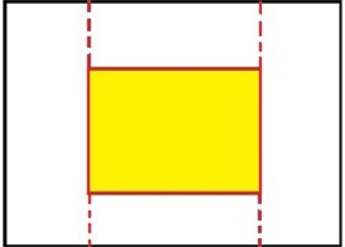
The domain Ω

However, 9 rectangles are required for a conforming decomposition. We mean by conforming that if the intersection of two rectangles Ω_i and Ω_j, i ≠ j is not empty, it is necessarily equal to a corner or to a hole edge of Ω_i and Ω_j.

We suppose that the intersection of each boundary ∂Ω_i of the sub-domain Ω_i with the boundary ∂Ω of the domain Ω is a corner or a hole edge of Ω_i. The skeleton of the decomposition

S=⋃i=1I∂Ωi∖∂Ω

is equal to

S¯=⋃m=1Mym¯,ym∩ym′=∅,1≤m≠m′≤M, (14)

where y_m is called mortar, which is equal to a hole edge of one sub-domain Ω_i that we note Ω_i(m). Let ℙ_{N_i}(Ω_i), N_i ≥ 2, 1 ≤ i ≤ I, the space of the polynomial functions defined on Ω_i, with degree ≤ N_i, for the two variables x and y.

We define the mortar discrete space 𝕏_δ, (δ = (N₁, …, N_I) is the discretization parameter) as the space of functions u_δ such that (see [7]):

u_{δ_{/Ω_i}}, 1 ≤ i ≤ I, belongs to the polynomial space ℙ_{N_i}(Ω_i),
u_δ vanishes on the boundary ∂Ω,
let ϕ the mortar function such that ϕ_{/y_m} = u_{δ_{/Ω_i(m)/y_m}}, for each Ω_i, 1 ≤ i ≤ I and an edge Γ of Ω_i, which is not included on the boundary ∂Ω, we have the following matching condition:

∀χδ∈PNi−2(Γ),∫Γ(uδ/Ωi−ϕ)(ξ)χδ(ξ)dξ=0, (15)

where ℙ_{N_i–2}(Γ) is the space of polynomials with degree ≤ (N_i – 2), defined on Γ. Since Γ does not always coincide with a mortar y_m, 1 ≤ m ≤ 𝓜, this allows us to say that the discretization is not conforming (𝕏_δ is not a subspace of H¹(Ω)).

We remind the Gauss-Lobatto quadrature formula on the interval Λ = ]–1, 1[:

If N ≥ 2 is an integer, let ϵ₀ = –1 and ϵ_N = 1, there exists a unique set of nodes ϵ_k, 1 ≤ k ≤ (N – 1) and weights ϱ_k, 0 ≤ k ≤ N, such that:

∀ψ∈P2N−1(Λ),∫−11ψ(ξ)dξ=∑k=1Nψ(ϵk)ϱk. (16)

Hereinafter, We recall the following property (see [11]):

∀κN∈PN(Λ),∥κN∥0,Λ2≤∑k=0NκN2(ϵk)ϱk≤3∥κN∥0,Λ2. (17)

We find the value of the nodes and weights ϵikx and ϱikx (respectively ϵiky and ϱiky ) in the direction x (respectively in the direction y) by homothety and translation of the domain Ω_i to the reference domain Λ². So, we have the discrete scalar product defined as:

For φ and ψ continuous on each Ω_i, 1 ≤ i ≤ I

(φ,ψ)δ=∑i=1I(φ,ψ)Ni, (18)

where

(φ,ψ)Ni=∑k=0Ni∑l=0Niφ(ϵikx,ϵily)ψ(ϵikx,ϵily)ϱikxϱily.

Let ∣φ∣d,Ω=(φ,φ)δ12 the associate discrete norm.

We introduce the auxiliary space

Yδ={κδ∈L2(Ω);κδ/Ωi∈PNi(Ωi);1≤i≤I}

and ℑ_δ the Lagrange interpolation operator defined as:

For all φ ∈ 𝕏_δ such as φ_{/Ω_i}, 1 ≤ i ≤ I is continuous on Ω_i, ℑ_δ(φ) ∈ 𝕐_δ, with Iδ(φ)(ϵikx,ϵily)=φ(ϵikx,ϵily).

We suppose for any 0 ≤ n ≤ M, fⁿ is continuous on each sub-domain Ω_i, 1 ≤ i ≤ I. Then we define the discrete problem:

Find uδn ∈ 𝕏_δ for each 1 ≤ n ≤ M, such that

uδ0=Iδ(u0),

and

∀vδ∈Xδ,aδn(uδn,vδ)=Lδn(vδ). (19)

The bilinear form aδn (., .), and the linear form Lδn (.), for 1 ≤ n ≤ M are defined as:

aδn(uδn,vδ)=(uδn,vδ)δ+τ∑i=1Iλi(∇uδn,∇vδ)Ni (20)

and

Lδn(vδ)=(uδn−1,vδ)δ+τ(fn,vδ)δ. (21)

Since the discretization is not conforming, we define the broken energy norm on 𝕏_δ

∥vδ∥Xδ=(∥vδ∥0,Ω2+τ∑i=1Iλi∣vδ∣1,Ωi2)12. (22)

Lemma 1

There exist two constants c₁ and c₂ independent of δ such that for all v_δ in 𝕏_δ, we have the following equivalence:

c1min(1,λmin)∑i=1I∥vδ∥1,Ωi2≤∥vδ∥Xδ≤c2max(1,λmax)∑i=1I∥vδ∥1,Ωi2. (23)

Proof

From (22) we deduce that

(∥vδ∥0,Ω2+τλmin∑i=1I∣vδ∣1,Ωi2)12≤∥vδ∥Xδ≤(∥vδ∥0,Ω2+τλmax∑i=1I∣vδ∣1,Ωi2)12.

We conclude (23) since

(∑i=1I∣vδ∣1,Ωi2)12and(∑i=1I∥vδ∥1,Ωi2)12

are equivalent with constants c₁ and c₂ independent of δ (see [12]).□

We prove using (17), Cauchy-Schwarz inequality and lemma 1 that the bilinear form aδn (., .) is continuous on 𝕏_δ × 𝕏_δ, coercive on 𝕏_δ and that the linear form Lδn (.) is continuous on 𝕏_δ. Using the Lax Milgram theorem, we obtain the following result.

Theorem 1

For f continuous on Ω×[0, T] and u₀ continuous on Ω, problem (19) has a unique solution (uδn)0≤n≤M in 𝕐_δ × (𝕏_δ)^M such that

∥uδn∥0,Ω2+τ∑j=1n∑i=1Iλi∥∇uδj∥0,Ωi≤9∥INu0∥0,Ω2+81C2λmaxλmin∑j=1n∥INfj∥0,Ω

where C is the Poincaré-Friedrichs constant which only depends on the domain Ω.

Proof 1

Let v_δ = uδn in problem (19). Using the Cauchy-Schwarz inequality, we have

|uδn|d,Ω2+τ∑i=1Iλi|∇uδn|d,Ωi2≤|uδn−1|d,Ω|uδn|d,Ω+|INfn|d,Ω|uδn|d,Ω.

Using (17), Poincaré-Friedrichs inequality and the fact that ab≤a22μ+μb22,∀μ>0

12|uδn|d,Ω2+τ∑i=1Iλi∥∇uδn∥0,Ωi2≤|uδn−1|d,Ω22+9∥INfn∥0,Ω22μ+λmax9C2μ2λmin∑i=1Iλi∥∇uδn∥0,Ωi2,

where C is the Poincaré-Friedrichs constant.

Doing the sum on n and using (17)

12∥uδn∥0,Ω2+τ∑j=1n∑i=1Iλi∥∇uδj∥0,Ωi2≤9∥INu0∥0,Ω22+92μ∑j=1n∥INfj∥0,Ω2+λmax9C2μ2λmin∑j=1n∑i=1Iλi∥∇uδn∥0,Ωi2.

Then we conclude by choosing μ=λmin9C2λmax.

5 Error estimate

For 1 ≤ n ≤ M, we recall that uⁿ is the solution of problem (7). In the case where λ is piecewise constant, problem (7) is written:

un+τλΔun=un−1+τfn inΩun=0 on∂Ωu0=u0 inΩ. (24)

Multiplying the first equation in (24) by v_δ ∈ 𝕏_δ and integrating by parts gives

an(un,vδ)=Ln(vδ)+∑i=1I∫∂Ωiλi(∂niun)vδdξ,

where n_i is the unit normal vector to ∂Ω_i.

If we define [v_δ] the jump of v_δ through the skeleton S, we obtain

an(un,vδ)=Ln(vδ)+12∫Sλ(∂nun)[vδ]dξ. (25)

Proposition 5

If f and u⁰ are respectively continuous on Ω × [0, T] and Ω, then the error estimate between (uⁿ)_0≤n≤M ∈ L²(Ω) × ( H01 (Ω))^M solution of (8) and (uδn)0≤n≤M∈Yδ×(Xδ)M solution of (19) is

∥un−uδn∥n≤c(infvδn∈Xδ∥un−vδn∥n+[infvδ0∈Yδ∥u0−vδ0∥0,Ω+λmaxλmin∑j=1n(Ea1,j+Ea2,j+Efj+Ecj)]) (26)

where

Ea1,j=1τsupwδ∈Xδ∫Ω(uj−uj−1)(x)wδ(x)dx−(vδj−vδj−1,wδ)δ∥wδ∥xδ,Ea2,j=supwδ∈Xδ∑i=1Iλi(∫Ωi∇uj∇wδdx−(∇vδj,∇wδ)Ni)∥wδ∥Xδ,Efj=supwδ∈Xδ∫Ωfj(x)wδ(x)dx−(f,wδ)δ∥wδ∥Xδ,Ecj=supwδ∈Xδ∫Sλ∂nuj[wδ]dξ∥wδ∥Xδ

and c is a positive constant independent of δ.

Proof 2

Let (vδn)0≤n≤M∈Xδ. By triangular inequality

∥un−uδn∥n≤∥un−vδn∥n+∥vδn−uδn∥n.

To estimate the term ∥uδn−vδn∥n, we consider the two problems (25) and (19) for w_δ ∈ 𝕏_δ:

∫Ωun(x)wδ(x)dx+τ∑i=1Iλi∫Ωi∇un(x)∇wδ(x)dx=∫Ωun−1(x)wδ(x)dx+τ∫Ωfn(x)wδ(x)dx+12∫Sλ∂nun[wδ]dξ

and

(uδn,wδ)δ+τ∑i=1Iλi(∇uδn,∇wδ)Ni=(uδn−1,wδ)δ+τ(fn,wδ)δ.

By doing the difference term by term, we obtain

(uδn−vδn,wδ)+τ∑i=1Iλi(∇(uδn−vδn),∇wδ)Ni=(uδn−1−vδn−1,wδ)δ+τLn(wδ)

where

Ln(wδ)=1τ[∫Ω(un−un−1)wδdx−(vδn−vδn−1,wδ)δ]+∑i=1Iλi(∫Ωi∇un∇wδdx−(∇vδn,∇wδ)Ni)+∫Ωfnwδdx−(fn,wδ)δ+12∫Sλ∂nun[wδ]dξ.

We remark that 𝓛ⁿ is linear and continuous on 𝕏_δ which is an Hilbert space for the scalar product (., .)_δ. Then, by Riesz theorem, there exists a unique element gδn ∈ 𝕏_δ such that

Ln(wδ)=(gδn,wδ)δ.

Therefore, we conclude that zδn=uδn−vδn is solution to problem (8) with a data function equal to gδn and zδ0 = ℑ_δu₀ – vδ0 . Consequently using theorem 1, we have

∥uδn−vδn∥n≤c∥Iδu0−vδ0∥0,Ω2+λminλmax∑j=1n∥gδj∥0,Ω21/2.

We remark that

∥gδj∥0,Ω≤csupwδ∈Xδ(gδj,wδ)δ∥wδ∥Xδ,

which permits to conclude (26).

Let for each mortar y_m ⊂ S, 1 ≤ m ≤ 𝓜, ζ(m) is the set of subscripts i, 1 ≤ i ≤ I, such that ∂Ω_i ∩ y_m has a positive measure. By estimating each term in (26), we obtain the following result proved in section 6.

Theorem 2

For λ constant on each Ω_i, 1 ≤ i ≤ I. Let f such that f_{/Ω_i} ∈ 𝓒⁰(0, T; H^σ_i(Ω_i));

σ_i > 1, u₀ is such that u_{0_{/Ω_i}} ∈ H^μ_i(Ω_i);μ_i > 1 and the solution (uⁿ)_0≤n≤M of problem (8) is such that u/Ωin ∈ H^s_i+1(Ω_i); s_i ≥ 0. Then the error between (uⁿ)_0≤n≤M and (uδn)0≤n≤M solution of problem (19) is

∥un−uδn∥n≤cτ[(1+β+βδ)λmaxλmin∑i=1IλiNi−2silog(Ni)∥un∥si+1,Ωi21/2+1min(1,λmin)1/2∑i=1INi−2σi∥f∥C0(0,T;Hσi(Ωi))21/2+∑i=1INi−2μi∥Iδu0∥μi,Ωi21/2], (27)

where c is a positive constant independent of δ,

β=max1≤m≤Mmaxk∈ζ(m)λkλi(m)1/2

and

βδ=max1≤m≤Mmaxk∈ζ(m)λkNi(m)λi(m)Nk1/2.

Remark 2

For a conforming decomposition, the term β_δ vanishes. Since there is no restriction on choosing of mortars, we opt, if it is possible, for those leading to

∀k∈ζ(m),λk≤λi(m). (28)

Thus β ≤ 1. If it is not possible, we choose the mortars and the degrees of approximation polynomials such that

∀k∈ζ(m),λkNk−1≤λi(m)Ni(m)−1, (29)

which may force us to make a small change in the decomposition. So we can optimize the estimation (27) without forcing the conformity of the decomposition.

6 Annex

This section is devoted to the proof of theorem 2. We need to estimate each term in (26).

6.1 Estimation of Ea1,j

We pose κ^j = u^j – u^j–1. By remarking that ΠNi−11κj=vδj−vδj−1, we deduce that

Ea1,j≤∥κj−ΠNi−11κj∥0,Ω

where ΠNi−11 is the orthogonal projection from H¹(Ω) to P_{N_i–1}(Ω).

The approximation properties of the operator ΠNi−11 are well known (see [11], Theorem 7.3 or [13], Proposition 2.6). This permit to obtain

Ea1,j≤cNi−si∥κj∥si,Ωi,

where, κ^j ∈ H^s_i(Ω_i); for s_i ≥ 1.

6.2 Estimation of Ea2,j

Using the exactness of the quadrature formula for a polynomial of degree ≤ 2N – 1, we write:

∑i=1Iλi[∫Ωi∇uj∇wδdx−(∇vδj,∇wδ)Ni]=∑i=1Iλi[∫Ωi∇(uj−ΠNi−11uj)∇wδdx−(∇(vδj−ΠNi−11uj),∇wδ)Ni].

By the triangular and Cauchy-Schwarz inequalities, we obtain:

supwδ∈Xδ∑i=1Iλi[∫Ωi∇uj∇wδdx−(∇vδj,∇wδ)Ni]∥wδ∥Xδ≤cλmax[∑i=1I|uj−ΠNi−11uj|1,Ωi+|vδj−ΠNi−11uj|1,Ωi],

then we conclude by the properties of operator ΠNi−11 .

6.3 Estimation of Efj

Let Π_{N_i–1} the orthogonal projection from L²(Ω_i) to ℙ_{N_i–1}(Ω_i). We have by the exactness of the quadrature formula, for a polynomial of degree ≤ 2N_i – 1,

∫Ωfj(x)wδ(x)dx−(fj,wδ)δ=∑i=1I[∫Ωi(fj−ΠNi−1fj)(x)wδ(x)dx−(Iδfj−ΠNi−1fj,wδ)Ni]

for all w_δ ∈ 𝕏_δ.

Using (17) in each direction, we obtain

∫Ωfj(x)wδ(x)dx−(fj,wδ)δ≤[10(∑i=1I∥fj−ΠNi−1fj∥0,Ω2)1/2+9∥fj−Iδfj∥0,Ω2]∥wδ∥0,Ω.

Using lemma 1 to bound ∥w_δ∥_0,Ω by ∥w_δ∥_{𝕏_δ} and the approximation properties of operator Π_{N_i–1} (see [11], Theorem 7.1) and ℑ_δ (see [11], Theorem 14.2) for f^j ∈ H^σ_i(Ω_i); σ_i > 1, we obtain

supwδ∈Xδ∫Ωfj(x)wδ(x)dx−(fj,wδ)δ∥wδ∥Xδ≤c(1min(1,λmin))1/2(∑i=1INi−2σi∥fj∥σi,Ωi2)1/2.

6.4 Estimation of Ecj

Let the operator

∂λnu/∂Ωi=λi∂niu,1≤i≤I.

This operator is discontinuous through the skeleton S. It means that if Γ = ∂Ω_i ∩ ∂Ω_i′, 1 ≤ i < i′ ≤ I, we have

∂λnu/∂Ωi+∂λnu/∂Ωi′=0 on Γ.

Lemma 2

For u^j in 𝕏_δ, 1 ≤ j ≤ n, such that u/Ωij∈Hsi+1(Ωi);si>0, we have:

supwδ∈Xδ∫S∂λnuj[wδ]dξ∥wδ∥Xδ≤c(1+β)∑i=1IλiNi−2si(log(Ni))∥uj∥si+1,Ωi21/2

where β=max1≤m≤Mmaxk∈ζ(m)λkλi(m)1/2 and c is a positive constant independent of δ.

Proof 3

Let ψ the mortar function associated to w_δ ∈ 𝕏_δ. By the matching condition (15), for each edge Γ of ∂Ω_i, 1 ≤ i ≤ I which is not mortar, we have:

∫Γ∂λnuj[wδ]dξ=λi∫Γ(∂niuj−πNi−2Γ∂niuj)(wδ/Ωi−ψ)dξ

where πNi−2Γ is the projection operator on ℙ_{N_i–2}(Γ).

We suppose now that the decomposition is conforming, then Γ = Ω_i ∩ Ω_i′, 1 ≤ i ≠ i′ ≤ I. We know that u/Ωij∈Hsi+1(Ωi), we study the two following cases.

If 0 < s_i < 12 , we define the trace of λ_i ∂_{n_i} u^j by duality:

For v ∈ H^1/2–s_i(Γ)

∫Γλi∂niujvdξ=λi∫ΩiΔujv~(x)dx+λi∫Ωi∇uj∇v~dx

where ṽ is the lifting function in H^1–s_i(Ω_i) of v.

Therefore, since πNi−2Γ is the orthogonal operator from H^s_i–1/2(Ω_i) into ℙ_{N_i–2}(Γ), we conclude then for any w_{N_i–2} and ψ_{N_i–2} in ℙ_{N_i–2}(Γ),

∫Γ∂λnuj[wδ]dξ≤∥λi1/2∂niuj∥si−1/2,Γλi1/2[∥wδ−wNi−2∥1/2−si,Γ+∥ψ−ψNi−2∥1/2−si,Γ].

Thus, the approximation properties (see [11]) allows us to deduce

∫Γ∂λnuj[wδ]dξ≤cNi−si∥λi1/2∂niuj∥si−1/2,Γλi1/2[∥wδ∥1/2,Γ+∥ψ∥1/2,Γ].

We remark that ∥w_δ∥_1/2,Γ is bounded by ∥w_δ∥_{1,Ω_i} and since the decomposition is conforming, ∥ψ∥_1/2,Γ is bounded by ∥w_δ∥_{1,Ω_i′} which permit to conclude.
In the case where s_i > 12 , we define πNi−2Γ the orthogonal projection operator from L²(Γ) to ℙ_{N_i–2}(Γ), then

∫Γ∂λnuj[wδ]dτ≤∥λi1/2(∂niuj−πNi−2Γ(∂niuj))∥0,Γλi1/2[∥wδ/Ωi−wNi−2∥0,Γ+∥ψ−ψNi−2∥0,Γ].

We conclude thanks to the approximation properties of πNi−2Γ (see [11], theorem 6.1).

The estimation in the case s_i = 1/2 is given by interpolation argument. In the case where Γ = ∂Ω_i ∩ ∂Ω, the mortar function ψ ∉ H^1/2(Γ) and a modification make appears (log(N_i))^1/2 ([13], proposition 21).

Remark 3

The term (log(N_i))^1/2 is negligible compared to Ni−si when N_i is big enough. This term disappears when the edges of any sub-domain Ω_i, 1 ≤ i ≤ I, which are not a mortar, are in the boundary ∂Ω.

6.5 Estimation of infvδn∈Xδ∥un−vδn∥n

Lemma 3

Let uⁿ ∈ 𝕏_δ; 1 ≤ n ≤ M such that u/Ωin ∈ H^s_i+1(Ω_i), s_i ≥ 2, then we have

infvδn∈Xδ∥un−vδn∥n≤c(1+β+βδ)∑i=1IλiN−2si∥un∥si+1,Ωi21/2

where c is a positive constant independent on δ and

βδ=max1≤m≤Mmaxk∈ξ(m)λkNi(m)λi(m)Nk1/2

depends on δ.

Proof 4

The proof will be done in three steps to construct vδn ∈ 𝕏_δ which represents the best approximation of uⁿ in the space 𝕏_δ.

Let πN0 the operator from H^3/2(Λ) in ℙ_N(Λ) which preserves ±1 (see [11], theorem 6.4), then ∀φ ∈ H^s(Λ), s ≥ 3/2 and 0 ≤ t ≤ 3/2,

∥φ−πN0φ∥t,Λ≤cNt−s∥φ∥s,Λ.

Let πNi0 the operator defined from πN0 by translation and homothety. We choose vδn1 such that

vδn1/Ωi=(πNi0,x∘πNi0,y)(u/Ωin),

where πNi0,x and πNi0,y are the operators in the x- and y-directions on Ω_i. We conclude then, if s_i ≥ 2 (see [11]):

λi1/2∥un−vδn1∥t,Ωi≤cλi1/2Nit−si−1∥un∥si+1,Ωi, (30)

where the function vδn1 vanishes on ∂Ω and coincides with uⁿ at the corners of the sub-domain Ω_i, 1 ≤ i ≤ I.
Let ϖ the set of vertices of Ω_i which are not a boundary of an edge of an other sub-domain Ω_i′. For c ∈ ϖ, ζ(c) is the set of subscripts i, 1 ≤ i ≤ I such that c ∈ ∂Ω_i. We denote by i(c) the index of ζ(c) such that

∀i∈ζ(c);λi≤λi(c)

and for i ∈ ζ(c)/{i(c)}, we define ψic the polynomial of minimal degree such that ψic (c) = 1 and vanishes on the edges of Ω_i which do not contain c and on the other points of ϖ ∩ ∂Ω_i, then:

vδn2=∑c∈ϖ∑i∈ζ(c)/{i(c)}vδ1n/Ωi(c)−vδ1n/Ωi(c)ψic.

So, we have for 0 ≤ t ≤ 3/2

λi1/2∥vδn2∥t,Ωi≤cλi1/2∑c∈ϖ∩∂Ωivδ1n/Ωi(c)−vδ1n/Ωi(c)≤cλi1/2∑c∈ϖ∩∂Ωi∥un−vδn1∥L∞(Ωi)+∥un−vδn1∥L∞(Ωi(c)).

Thanks to the Gagliardo-Nirenberg inequality, for 0 < α_i < 1/2

λi1/2∥vδn2∥t,Ωi≤cλi1/2(∑c∈ϖ∩∂Ωi∥un−vδn1∥1−αi,Ωi1/2∥un−vδn1∥1+αi,Ωi1/2+∥un−vδn1∥1−αi,Ωi(c)1/2∥un−vδn1∥1+αi,Ωi(c)1/2

Since λ_i ≤ λ_i(c) and using (30) (for t = 1 – α_i and t = 1 + α_i), we conclude that:

λi1/2∥vδn2∥t,Ωi≤cλi1/2Ni−si∥un∥si+1,Ωi+∑c∈ϖ∩∂Ωiλi(c)1/2Ni−si(c)∥un∥si(c)+1,Ωi(c). (31)

Therefore, we end by doing the sum on i, 1 ≤ i ≤ I.
Let 𝓗_i, 1 ≤ i ≤ I the set of edges of Ω_i which are not include in ∂Ω and are not mortars.

If φ is the mortar function associated to vδn1+vδn2, then

vδn3=∑i=1I∑Γ∈HiRiLπNiΓ∗φ−(vδn1+vδn2)/Ωi

where

RiL is the lifting operator from ℙ_{N_i}(Γ) ∩ H001/2 (Γ) into ℙ_{N_i}(Ω_i), such that ∀φ_δ ∈ ℙ_{N_i}(Γ) ∩ H001/2 (Γ) (see [14])

∥RiLφδ∥1,Ωi≤c∥φδ∥H001/2(Γ), (32)
πNiΓ∗ is the operator of projection from H001/2 (Γ) to ℙ_{N_i}(Γ) ∩ H001/2 (Γ), such that ∀φ ∈ H001/2 (Γ)

∫Γ(φ−πNiΓ∗φ)ψδ(τ)dξ=0∀ψδ∈PNi−2(Γ). (33)

Then following (31)

λi1/2∥vδn3∥1,Ωi≤cλi1/2∑Γ∈Hi∥πNiΓ∗φ−(vδn1+vδn2)/Ωi∥H001/2(Γ).

Since πNiΓ∗φ−(vδn1+vδn2)/Ωi coincides with (vδn1+vδn2)/Ωi on Γ, then:

λi1/2∥vδn3∥1,Ωi≤cλi1/2∑Γ∈Hi(∥un−(vδn1+vδn2)H001/2(Γ)+∥(id−πNiΓ∗)un−(vδn1+vδn2)∥H001/2(Γ)) (34)

where [.] is the jump through Γ.

Using the trace theorem, (30) and (31), we conclude for t = 1 that

λi1/2∥un−(vδn1+vδn2)∥H001/2(Γ)≤λi1/2(Ni−si∥un∥si+1,Ωi+∑mes(∂Ωi∩ym)>0Ni(m)−si(m)∥un∥si(m)+1,Ωi(m)). (35)

To evaluate the second term in (34), we remark that the operator πNiΓ∗ is equal to the operator of projection from H01 (Γ) into ℙ_{N_i}(Γ) ∩ H01 (Γ). Then, ∀ψ ∈ H01 (Γ)

∥ψ−πNiΓ∗ψ∥H001/2(Γ)≤cNi−1/2∥un−(vδn1+vδn2)∥1,Γ.

Therefore, we proceed as before with t = 3/2, we obtain

λi1/2∥(id−πNiΓ∗)un−(vδn1+vδn2)∥H001/2(Γ)≤cλi1/2Ni−1/2(Ni1/2−si∥un∥si+1,Ωi+∑mes(∂Ωi∩ym)>0Ni(m)1/2−si(m)∥un∥si(m)+1,Ωi(m)). (36)

This is where we introduce β_δ.

To conclude the proof of Theorem 2, we choose vδn=vδn1+vδn2+vδn3 in 𝕏_δ and combine (30), (31), (35) and (36).

Conclusion

This work concerns the numerical analysis of the mortar spectral elements method discretization of the heat equation with a diffusion coefficient λ, depending on the heterogeneity of the domain. To solve the problem of the solution singularity due to the discontinuity of λ, we use a non conform geometric decomposition of the domain. We prove an optimal error estimate that depends only on the local regularity of the solution. The numerical validation of this result will be the subject of a forthcoming work.

Acknowledgments

The authors acknowledge funding from the Research and Development (R&D) Program (Research Pooling Initiative), Ministry of Education, Riyadh, Saudi Arabia, (RPI-KSU).

References

[1] N.S. Papageorgiou, V.D. Radulescu and D.D. Repovs, Nonlinear analysis – theory and methods, Springer Monographs in Mathematics. Springer, Cham, 2019.10.1007/978-3-030-03430-6Search in Google Scholar

[2] A. Bergam, C. Bernardi and Z. Mghazli, A posteriori analysis of the finite element discretization of some parabolic equations, Math. Comp. 74 (2005), no. 251, 1117-1138.10.1090/S0025-5718-04-01697-7Search in Google Scholar

[3] N. Chorfi, M. Abdelwahed and I. Ben Omrane, A posteriori analysis of the spectral element discretization of heat equation, An. St. Univ. Ovidius Constanta. 22 (3) (2014), 13-35.10.2478/auom-2014-0047Search in Google Scholar

[4] V. Thomée, Galerkin Finite Element Methods for Parabolic Problems, Springer Series in Computational Mathematics 25, Springer, Paris, 1997.10.1007/978-3-662-03359-3Search in Google Scholar

[5] C. Bernardi and R. Verfürth, Adaptive finite element methods for elliptic equations with non-smooth coefficients, Numer. Math. 85 (2000) 579-608.10.1007/PL00005393Search in Google Scholar

[6] C. Bernardi and N. Chorfi, Mortar spectral element methods for elliptic equations with discontinuous coefficients, Math. Models Methods Appl. Sci. 12 (2002), no. 4, 497-524.10.1142/S0218202502001763Search in Google Scholar

[7] C. Bernardi, Y. Maday and A. T. Patera, A new nonconforming approch to domain decomposition: the mortar element method, in Nonlinear Partial Differential Equations and their Applications, Collège de France Seminar, H. Brézis, J.-L. Lions, Eds, (1991).Search in Google Scholar

[8] B. I. Wohlmuth, Discretisation Methods and Iterative Solvers Based on Domain Decomposition, Lecture Notes in Computational Science and Engineering, Vol. 17 (Springer 2001).10.1007/978-3-642-56767-4Search in Google Scholar

[9] J. L. Lions and E. Magenes, Problèmes aux Limites non Homogène et Applications, 1, Dunod, (1968).Search in Google Scholar

[10] N. G. Meyers, An L^p-estimate for the gradient of solutions of second order elliptic divergence equations, Ann. Sci. Norm. Sup. Pisa 17 (1963) 189-206.Search in Google Scholar

[11] C. Bernardi and Y. Maday, Spectral Methods, in Handbook of Numerical Analysis V, P.G. Ciarlet and J.-L. Lions, eds., North–Holland, Amsterdam, 1997, pp. 209-485.10.1016/S1570-8659(97)80003-8Search in Google Scholar

[12] M. Azaïez, C. Bernardi and Y. Maday, Some tools for adaptivity in the spectral element method, in Proc. of Third Int. Conf. On Spectral And High Order Methods, Houston J. Math. (1996) 243-253.Search in Google Scholar

[13] C. Bernardi and Y. Maday, Spectral, spectral element and mortar element methods, in Theory and Numerics of Differential Equations, Durham 2000, eds. J. F. Blowey, J. P. coleman and A. W. Craig (Springer, 2001), pp. 1-57.10.1007/978-3-662-04354-7_1Search in Google Scholar

[14] C. Bernardi, M. Dauge, and Y. Maday, Polynomials in the Sobolev World, Internal Report, Laboratoire Jacques-Louis Lions, Université Pierre et Marie Curie, Paris, France, 2003.Search in Google Scholar

Received: 2019-05-06

Accepted: 2019-06-06

Published Online: 2019-10-16

This work is licensed under the Creative Commons Attribution 4.0 Public License.

Articles in the same Issue

https://doi.org/10.1515/anona-2020-0043

Keywords for this article

Elliptic equation; Discontinuous coefficient; Mortar spectral element method; Error analysis

Creative Commons

BY 4.0