The dichotomy between chemical concepts and numbers after almost 100 years of quantum chemistry: conceptual density functional theory as a case study

1 Introduction

The International Union of Pure and Applied Chemistry (IUPAC) has endorsed the celebration of the year 2025 as the International Year of Quantum Science and Technology. By editing a Special Issue of Pure and Applied Chemistry, the official journal of IUPAC, it pays tribute, as the worldwide organization of Chemists, to the importance and achievements of Quantum Science in the field of Chemistry. Quantum mechanics, the most fundamental branch of quantum science and technology which is at the basis of their development, emerged in the first quarter of the 20th century. Brilliant physicists like Planck, Einstein, Bohr, Heisenberg, Schrödinger, Dirac and many others reshaped our thinking and understanding of the world by a rigorous description of the behavior of the (at that time) most elementary particles at atomic and subatomic scales.

Physics it was, at the highest possible level, but some aspects of deep interest for chemists already appeared. Both in the old (Bohr) and the new (Schrödinger) quantum theory, the properties of the hydrogen atom, the simplest atom of all, were treated in detail culminating in the explanation of the frequencies and intensities of the Hydrogen spectrum. The extension to heavier atoms, starting with Helium, though technically more intricate, was ahead with the Periodic Table, the ultimate playground of the chemists, as a possible goal on the longer term. Remarkably, very soon after the fundamentals of quantum mechanics were casted in Schrödinger’s celebrated equation in 1925, two sets of papers were published only two years later which already took the step to the chemist’s beloved molecular world and in which the still mysterious chemical bond plays a decisive role. Heitler and London ¹ on one hand and Hund on the other hand ² presented successful but alternative treatments of the hydrogen molecule. Both approaches were soon after extended/refined by others and are now known as the Heitler-London-Slater-Pauling ^{1 , 3 , 4} vs. the Mulliken-Hund ^{2 , 5} or the Valence Bond vs. the Molecular Orbital Theories, their differences needing no further explanation for this readership. An authoritative review of these first years of what Quantum Chemistry in “statu nascendi” was can be found in Mary Jo Nye’s extensive treatise “From Chemical Philosophy to Theoretical Chemistry”. ⁶

In this treatise the author refers to a quote by Coulson ⁷ claiming that the development of wave mechanics from Schrödinger to Dirac came to a “full stop about 1929 insofar as chemistry was concerned” and cites Hirschfelder stating that “At this point, the theoretical physicists left the chemist to wallow around with their messy molecules while they resumed their search for new fundamental laws of nature”. ⁸

Chemists started to take up the challenge and Pauling’s contribution in this endeavor is hard to overestimate with his quantum-mechanical explanation of directed valence and the introduction of the hybridization concept in his famous 1931 paper. ^{4 , 9} Almost 100 years later this concept is still a basic tool when rationalizing the structure and properties of molecules. In the same period and in the spirit of the Hund-Mulliken approach, Hückel launched a simple but insightful ansatz to investigate unsaturated organic molecules by using an expansion of (π) molecular orbitals in a series of atomic basis functions. ¹⁰ This formed the basis of Longuet-Higgins’ and Coulson’s lasting series of papers on “The Electronic Structure of Conjugated Systems”. ¹¹ It is the authors’ humble opinion that one can say that around 1935 Quantum Chemistry has already matured to a branch of science embedded in chemistry. Indebted in its basic approach to quantum physics it envisaged explaining/interpreting facts and concepts from chemistry on the basis of the fundamental laws of nature as laid down in quantum mechanics. The qualitative aspect was still preponderant at that time, the quantitative one, except for few electron systems, still being out of reach.

This aspect is reflected in the first edition of Coulson’s “Valence” in 1952 ¹² which had an enormous impact on chemistry. It showed that, even with a moderate mathematical machinery, chemists may grasp a better understanding of fundamental concepts in chemistry through Quantum Mechanics. The book has known continuing success in later editions, finally taken care of by Mc Weeny. ¹³

In the same vein we refer to the famous after dinner speech, again by Charles Coulson, at the banquet of the Boulder Conference in Molecular Quantum Mechanics in 1959. In a masterly formulated state-of-the-art address, he reflected on the evolution of the discipline since the pre-war period. ¹⁴ Referring to the quantitative aspect Coulson points to the bottleneck of the efficient evaluation of many-center integrals in the endeavor to get accurate numbers for polyatomic molecules. However electronic computers were becoming developed commercially to the stage where it became feasible to program large scale computations. But… he also insists on the importance of explaining things stating that “…any explanation must be given in terms of concepts which are regarded as adequate or suitable”. When a calculation exactly reproduces an experimental fact, he does not consider that as an explanation but merely a confirmation of the experiment. Everywhere in the literature the quotation to this talk is found as “Give us insight, not numbers”.

Ever since then an astonishing evolution has taken place in what Coulson called ab initio quantum chemistry, at that time restricted however to systems with a small number of electrons. Nowadays, thanks to the combination of more and more performant theoretical approaches (first in wave function theory, later (vide infra) in Density Functional theory) and increasing computing power, overall trustworthy numerical results can be obtained and even chemical accuracy (1 kcal mol⁻¹) can be reached for larger and larger systems. Nevertheless, many chemists, both theoreticians and certainly experimentalists, are mainly interested in understanding what comes out of these impressive calculations and in translating the results into their common language of bonds, hybridization, aromaticity, atomic charges… which is not always evident. There a possible disadvantage of these high-level calculations shows up because, as Mulliken already stated in 1965, “the more accurate the calculations became the more the concepts tended to vanish in the air”. ¹⁵

However, a variety of interpretational techniques have been put forward coping at least partially with this issue and in 2019 Neese and coworkers wrote an interesting paper where they challenged Coulson’s dictum turning it into “Give us Insight and Numbers”. ¹⁶ Concentrating on wave function-based approaches they argue that nowadays accurate first principle calculations can be performed on large molecular systems while tools are available to interpret the results of these calculations in chemical language. They support their claim by giving a few well-chosen examples of interpretational techniques applied to high level computational results in organic, inorganic, organometallic and surface chemistry among others the Local Energy Decomposition ¹⁷ (referring also to the Natural Bond Analysis (NBO), ¹⁸ and the Quantum Theory of Atoms in Molecules (AIM) ¹⁹ ) and ab initio Ligand Field Theory (AILFT). ²⁰ By introducing “numbers” in Coulson’s statement (for which they also refer to Gernot Frenking’s talks) these numbers should in their opinion however not be viewed as the sole and ultimate goal of a theoretical investigation. The chemical “insights” that arise from them are at least as important as they fulfill one of the most important missions of the theory, namely to inspire and guide new experiments.

The present authors fully agree with this statement but would in this contribution address two additional points emerging from their own experience

1. The arguments of Neese and coworkers of course give rise to the question; which interpretational methods are advisable to be used, thereby remaining as closely as possible to traditional chemical concepts but casted in a systematic framework?

2. When defined, is there a unique, optimal way to evaluate these quantities, or are they themselves not subjected to important numerical variations when they are for example treated at different levels of approximation, thereby blurring their broad and systematic use?

These issues will be dealt with in the context of Conceptual Density Functional Theory (CDFT), ^{21 , 22 , 23 , 24 , 25 , 26 , 27 , 28 , 29 , 30} a sub-branch of Density Functional Theory (DFT) ^{31 , 32} which has as primary objective to develop a nonempirical, mathematically and physically sound, density-based, quantum-mechanical theory for interpreting and predicting chemical phenomena, especially chemical reactions. In the past decades this approach, initiated by Robert Parr in the late 1970s, ³³ has turned out to be valuable in the interpretation of both wave function and DFT computational results whatever their level of theory (thus coping with Mulliken’s remark), as well as experimental data. A restricted number of chemical concepts are thereby introduced in a unified and mathematically sound framework. Most of them are related to, or an extension of, existing but sometimes vaguely defined concepts. Response functions, ^{29 , 34 , 35} originating in theoretical physics, thereby play a fundamental role, quantifying the propensity of an atom, molecule, complex… to respond to perturbations in its number of electrons and/ or their external potential, as provoked by e.g. a second reagent.

The question then of course arises how to evaluate these quantities as accurately as possible in order to refine our insight. It is at this moment that a new confrontation “insight vs. numbers” appears because as will be seen from our case studies it may be possible that upon refinement either minor influences show up, but that also fundamental issues arise hidden in the definition and the background of the response functions. To put it otherwise it is worth investigating if when trying to get insight, numbers are also, and in some cases strongly, at stake. This question will be addressed in the context of recent work in our group on efforts to refine the evaluation of CDFT based concepts, thereby proceeding to their analytical evaluation. ^{36 , 37 , 38 , 39 , 40}

In Part 2 of this paper a brief introduction to Conceptual DFT will be given, concentrating on the nature and relevance of these response functions by linking them to classical chemical concepts, thereby answering the first question formulated above. In Part 3 we will show how, once defined, their evaluation can be achieved, yielding numbers but also how these numbers display a different behavior upon refining their evaluation. The three examples considered, the linear response function (3.1), ^{21 , 34 , 36 , 41} the Fukui function (3.2) ^{38 , 42 , 43} and the hardness (3.3) ^{38 , 44 , 45} will be shown to behave differently under refinement thus (partly) answering the second question formulated above.

2 The very basics of conceptual density functional theory: response functions

Density Functional Theory (DFT) ²¹ was recently termed the workhorse of quantum chemistry and materials science. ⁴⁶ This theory was formally established by the two Hohenberg–Kohn theorems, ³¹ justifying the use of the electron density ρ(r) of the system as the basic variable instead of the wavefunction Ψ.

The first Hohenberg–Kohn theorem provides justification for writing the ground state energy E of an atomic, molecular or solid state system and its different components as so-called functionals of its electron density, i.e.

with T[ρ(r)] the kinetic energy, V _ne[ρ(r)] the nucleus-electron attraction energy and V _ee[ρ(r)] the electron-electron repulsion energy density functionals. In the second part of this equation, the so-called Hohenberg–Kohn functional F _HK[ρ(r)] has been introduced collecting the T[ρ(r)] and V _ee[ρ(r)] contributions.

The second Hohenberg–Kohn theorem establishes a variational principle allowing the use of the electron density to obtain the ground state energy of the system: mimimizing the system’s energy with respect to changes in the electron density will yield the ground state energy and electron density of the system. Application of this variational principle, i.e. minimizing the energy of the system with respect to changes in the electron density with the constraint that the density during this process should always integrate to the number of electrons N of the system, yields

In this equation, μ is the Lagrange multiplier attached to the density normalization constraint. Working out this equation ultimately yields the following equation which can be termed the DFT analogue of the Schrödinger equation, i.e.

The exact functional form of F _HK[ρ(r)] is unknown and its magnitude is large, so even the smallest errors in its approximation lead unacceptably large errors when using this equation for determining the energy of chemical systems. To circumvent this problem, Kohn and Sham re-introduced orbitals considering a non-interacting reference system with an electron density exactly equal to the density of the true system. ³² For such a non-interacting system with N electrons, the kinetic energy, denoted as T _s , can be written exactly as

The other term in the Hohenberg–Kohn functional, the electron-electron repulsion of the system, is then written as the classical Coulomb self-repulsion J ρ r and a correction term. This results in the following expression for F _HK[ρ(r)]

with E _XC[ρ(r)] the so-called exchange-correlation energy

This results in the following expression of the Kohn–Sham energy functional

Minimization of this Kohn–Sham energy with respect to the occupied orbitals in the non-interacting reference system now gives rise to the Kohn–Sham equations,

where ϵ _i are the Kohn–Sham orbital energies. v _KS(r) is the Kohn–Sham potential that has three contributions

The first term is the external potential of the system; for an isolated system (i.e. a system in the absence of external fields) this is the potential due to the nuclei i.e.

with M the number of nuclei in the system and Z _A the charge of nucleus A (in a.u.).

v J r is the classical Coulomb potential due to the electrons, i.e.

The last potential term, the only unknown term in the Kohn–Sham equations, is the functional derivative of the exchange correlation energy with respect to the electron density and is called the exchange-correlation potential.

Unfortunately, unlike wavefunction methods that have a well-defined path for convergence to the exact solution of the Schrödinger equation, the exchange-correlation functional is not systematically improvable. A possible organizing principle was put forward by Perdew, the so-called Jacob’s ladder. ⁴⁷ This ladder has its foundations in the Hartree world, where the exchange-correlation energy is zero and the electron-electron interaction if provided only by classical electrostatics, i.e. by J [ ρ r ]. When moving up this ladder, additional ingredients are introduced in the exchange-correlation functional form. “Heaven” is the elusive goal of the exact exchange-correlation functional (and thus the exact solution of the Schrödinger equation), i.e. the heaven of chemical accuracy. Jacob’s ladder is characterized by five rungs:

1. The Local Density Approximation (LDA): the simplest exchange-correlation functionals depend only on the electron density and define the first rung:

1. The generalized gradient approximation (GGA): these functionals include, next to the electron density, also the change of the density in space through the density gradient:

1. Meta GGAs: higher derivatives are included into the functional, namely the density laplacian ∇² ρ or the kinetic energy density τ = ∑ i | ∇ ψ i | 2

1. Hybrid functionals, where a fraction of Hartree–Fock exchange ( E X HF is mixed in. A so-called general hybrid has the following form:

E X DFT and E C DFT can be both GGA or meta-GGA type of functionals. Additionally, this category of exchange-correlation functionals also includes so-called range-separated functionals, where the electron-electron interaction is split into two parts: one long-range and the other short-range.

1. Double hybrid functionals: in these functionals, parts of conventional DFT exchange and correlation are replaced by contributions from nonlocal Hartree Fock-exchange and second-order perturbation theory. As a result, these functionals will also be dependent on the virtual orbitals of the system.

For a review of functionals of the first four rungs of Jacob’s ladder, see e.g. ⁴⁸ ; double hybrid functionals are reviewed in e.g. ⁴⁹

Analytical expressions for the conceptual DFT reactivity indices will be presented in this work using the first four of these rungs.

Through the Hohenberg–Kohn theorems, the ground state energy for a non-degenerate system is proven to be a unique functional of the electron density. Since the density of the system determines its number of electrons (through its integration over space) and its external potential (due to the first Hohenberg–Kohn theorem), the energy is a functional of N and v(r).

In CDFT, the propensity of a molecule to react with a given partner is governed by the change in its energy functional, E = E[N,v(r)], due to the perturbation in N and v(r) induced by the reaction partner and is written as a Taylor series expansion. Using the onset of the reaction as the reference the expansion coefficients or response functions are the partial and functional derivatives of the energy with respect to N and v(r), respectively, i.e., ∂ m δ m ′ E ∂ m N δ v r 1 … δ v r m ′ . ^{21 , 22 , 23 , 24 , 25 , 26 , 27 , 28 , 29 , 30} They measure the sensitivity of the system towards the perturbation or the intrinsic part (i.e. without consideration of the magnitude of the perturbation) of the response of the system and provide interesting chemical information about the system; these quantities can be collected in a so-called response function tree (Fig. 1). ^{23 , 24 , 29 , 34}

Fig. 1:

Response function tree from conceptual DFT up to third order. Reproduced with permission from Chapter 2 of Reference 30], Wiley-VCH, Weinheim Germany, 2022.

The lowest (i.e. first-order) response functions are directly related to fundamental quantities of DFT. From first order perturbation theory one proves that

i.e. the first order response of the energy with respect to a change in the external potential equals the central quantity in DFT, the electron density.

The electronic chemical potential, the Lagrangian multiplier in the variational DFT equation associated to the constraint of fixed electron-number, in turn equals the derivative of the energy with respect to the number of electrons N,

The breakthrough identification of this electronic chemical potential as the opposite of the electronegativity (often given the symbol χ) by Parr, Donnelly, Levy and Palke provided a clear link between DFT, CDFT and long standing chemical concepts.3 ³³ The evaluation of the chemical potential or the electronegativity requires the derivative of the energy with respect to the number of electrons. In a seminal paper, using an ensemble approach, Parr, Perdew, Levy and Balduz showed that the exact E versus N curve comprises a series of straight lines with derivative discontinuities at the integer N. ⁵⁰

Using a finite difference approximation, the μ and χ can be obtained as

where I and A are the vertical ionisation energy and electron affinity of the system. This expression equals the Mulliken definition for the electronegativity ⁵¹ and can also be retrieved when using a quadratic model for the energy versus the number of electrons.

Within a Koopmans type of approximation, ⁵² the electronegativity can be obtained as the average of the HOMO and LUMO orbital energies. ⁵³

We now progress to the higher N and v(r) derivatives in the response function tree and their identification with a variety of chemical concepts.

Parr and Pearson introduced the chemical hardness η as ⁴⁴

This quantity measures the system’s resistance to a charge transfer and, again within a finite difference approximation, can be expressed as

Using again a Koopmans type of approximation, the hardness equals

i.e. the HOMO-LUMO gap. The inverse of the global hardness is the global softness. ⁵⁴

The concept of chemical hardness (and softness) was introduced in the 1960s by Pearson; he proposed, based on a large collection of experimental thermochemical data, a classification of Lewis acids and bases as hard or soft and formulated the Hard and Soft Acids and Bases (HSAB) principle: Hard acids prefer to bond to Hard bases and Soft acids prefer to bond to Soft bases. ⁴⁵ Another CDFT principle involving the chemical hardness is the Maximum Hardness Principle, stating that there seems to be a rule of nature that molecules arrange themselves so as to be as hard as possible.5 ⁵⁵

The mixed derivative in the response function tree, ∂ δ E δ v r ∂ N , was defined by Parr and Yang as the Fukui function. ⁴²

This (local) reactivity index measures the change of the system’s electron density when changing the number of electrons of the system. It integrates to unity over space

Due to the discontinuity of the electron density derivative with respect to the number of electrons, a Fukui function can be defined both for the subtraction or addition of a fraction of an electron. The derivative of the electron density when subtracting a fraction of an electron is the Fukui function for an electrophilic attack, i.e.

In this equation, ρ _N(r) and ρ _N-1(r) are the electron densities of the N and N-1 electron systems respectively, obtained at the geometry of the N electron system (cf. the requirement of the evaluation of the derivative at constant external potential).

The Fukui function for a nucleophilic attack is given by density change upon addition of an electron

where ρ _N+1(r) is the electron density of the N+1 electron system, again evaluated at the geometry of the N-electron system.

For a radical attack, the Fukui function f ⁰(r) is introduced as the average of f ⁺(r) and f ⁻(r). When the exact electron densities of the N, N-1 and N+1 electron systems would be used, the expressions for f ⁻(r) and f ⁺(r) would be exact (i.e. the finite difference evaluation is exact).

Parr, Yang and Pucci derived expressions for the Fukui functions f ⁻(r) and f ⁺(r) in terms of the Kohn–Sham orbitals. For a system of M electrons (the M-th and M+1-th Kohn Sham orbital thus being the HOMO or LUMO respectively), the Fukui functions become ⁵⁶

and

As can be seen, the Fukui functions can be written as the frontier MO densities and a correction term probing orbital relaxation upon changing the number of electrons; these expressions connect CDFT to Fukui’s frontier MO concept.

Yang and Mortier introduced the atom-condensed Fukui functions by taking the difference of the atomic Mulliken populations of the atom in the N, N-1 and N+1 systems. As such, the Fukui functions condensed to an atom k, for an electrophilic, nucleophilic and radical attack are then obtained as ⁵⁷

and

where q _k (N), q _k (N+1) and q _k (N-1) are the atomic populations of atom k in the N, N-1 and N+1 electron system respectively.

Yang and Mortier originally used Mulliken populations to evaluate the condensed Fukui functions but also other population analysis schemes have been used for this purpose. Different condensation schemes will of course yield different numerical values of this quantity. ⁵⁸

The Fukui function describes density changes when changing the number of electrons of the system. As such, it describes a charge transfer contribution during a chemical reaction and can thus be linked to soft-soft (covalent) interactions. The local softness s(r) has been introduced as the product of the Fukui function and the global softness of the system ⁵⁹

The local softness thus gives the same intramolecular reactivity information as the Fukui function; it distributes the total softness of the molecule over the entire system. It can however be used to probe intermolecular reactivity.

One obtains the global softness of the system when the local softness is integrated over space

In analogy to the Fukui function, one can evaluate the local softness for a nucleophilic, electrophilic or radical attack by multiplying the global softness of the system with the appropriate Fukui function.

In this contribution, attention will be focused on the analytical evaluation of response functions up to second order, in particular the chemical hardness, the Fukui function and the linear response function. We do however mention here an important third order derivative, the dual descriptor f ⁽²⁾(r), introduced by Morell and co-workers. ^{60 , 61} This quantity, the derivative of the Fukui function with respect to the number of electrons, can provide a one-shot picture of the electrophilic and nucleophilic regions in the molecule

Coming back to the second order response functions, the last response function we will consider in this paper is the linear response function (or linear response kernel), the second functional derivative of the energy with respect the electron density, i.e. ^{21 , 34 , 36 , 41}

This quantity expresses how the electron density at a given point r changes following a change of the external potential at a point r’ (or vice versa). It is the static equivalent of the frequency dependent linear response function χ(r,r ^′,ω), an important quantity from time-dependent DFT. ⁶²

The theoretical and formal aspects connected to this quantity have been investigated in detail and additionally, it has proven to be a source of highly interesting chemical information, ^{63 , 64 , 65 , 66 , 67 , 68 , 69 , 70 , 71 , 72 , 73} such as e.g. the atomic shell structure, inductive and mesomeric effects, electron delocalization, aromaticity and anti-aromaticity, electrical conductivity, and the nearsightedness of electronic matter principle of Kohn and Prodan. ⁷⁴

3 Refining the evaluation of response functions: the three second order energy derivatives

3.1 The linear response function

3.1.1 Theory

As a first example, we now focus on the linear response function, whose evaluation, interpretation, visualization and application has been a central theme in the CDFT research of our group. ^{36 , 37 , 41 , 63 , 64 , 65 , 66 , 67 , 68 , 69 , 70 , 71 , 72 , 73}

The CDFT linear response function can be considered as an extension of the atom-atom polarizability from the Hückel level of theory. The atom-atom polarizability between atom r and atom s (π _r,s ) was defined by Coulson and Longuet-Higgins as ¹¹

(37) π s , r = ∂ q s ∂ α r = ∂ 2 E π ∂ α r ∂ α s = ∂ 2 E π ∂ α s ∂ α r = ∂ q r ∂ α s = π r , s

with q the π charge, α the Coulomb integral of the atom considered and E _π the total π energy.

In this section, we will discuss a number of examples and representations when this concept is refined from its form traditionally obtained using the independent particle approximation derived from a coupled-perturbed Kohn Sham computation.

For a closed shell system and starting from the coupled-perturbed Hartree–Fock (CPHF) or Kohn–Sham (CPKS) approach, the linear response function can be written as

(38) χ r , r ′ = δ ρ r δ v r ′ N = − 4 ∑ i a , j b M − 1 i a , j b φ i r φ a r φ j r ′ φ b r ′

where the indices i, j, k… are used for occupied and a, b, c… for virtual orbitals φ with corresponding orbital energies ε _i and ε _a respectively. This constitutes a generalization of Eq. (37), replacing E_π and α by the total energy and the external potential respectively. The M matrix in this expression is given by

in Hartree–Fock theory:

(39) M i a , j b H F = ε a − ε i δ i j δ a b + 4 i a | j b − K i a , j b

in Kohn–Sham DFT (LDA, GGA and meta-GGA):

(40) M i a , j b K S = ε a − ε i δ i j δ a b + 4 i a | j b + 4 i a | f x c r , r ′ j b

for Hybrid functionals:

(41) M i a , j b H Y B = ε a − ε i δ i j δ a b + 4 i a | j b − α K i a , j b + 4 i a | f x c r , r ′ ; α j b

for coulomb attenuated functionals (CAM): ⁷⁵

(42) M i a , j b C A M = ε a − ε i δ i j δ a b + 4 i a | j b − α K i a , j b S R − α + β K i a , j b L R + 4 i a | f x c r , r ′ ; α , β j b

with K i a , j b = i b | j a + i j | a b . K i a , j b S R and K i a , j b L R imply the short and long-range contribution of the exact exchange in which the numerator of the 1 r 12 operator is replaced by erfc(ω) and erf(ω), respectively, where ω the range-separation parameter. This separation of short- and long-range parts can also be extended to other range-separation forms. The integrals (pq|rs) are expressed in chemists’ notation, where the first two and the last two arguments have the same spatial variables. As can thus be seen, the Kohn–Sham evaluation of the LRF involves the first four rungs of Jacob’s ladder.

Considering how this M matrix is constructed, one can distinguish between three levels of approximation, both within Hartree–Fock and Kohn–Sham DFT:

1. the independent particle approximation (IPA):

(43) M ≈ ε a − ε i δ i j δ a b ;

This approximation has been used exclusively in the past to uncover the chemistry contained in the LRF.

1. the random phase approximation (RPA)

(44) M ≈ ε a − ε i δ i j δ a b + i a | j b

i.e. adding an extra Coulomb term (ia|jb) to the IPA approximation

1. the “full” expression within HF or DFT theory (HFA or DFT), considering the full set of matrix elements. This implies that the RPA level is extended with either HF exchange or the DFT exchange-correlation term, respectively, additionally taking into account the nature of the functional used (e.g. hybrid, CAM). In the case of Kohn–Sham DFT, the DFT exchange-correlation kernel is included in the expression of the M matrix: it is defined as f _xc ( r , r ^′) = δ ² E _xc /δρ( r )δρ( r ^′). For a LDA or GGA functional, it can be expressed as

(45) δ 2 E x c δ ρ r δ ρ r ′ = δ r − r ′ ∂ 2 e x c ∂ ρ ∂ ρ r ′ − ∇ p ∂ 2 e x c ∂ ∇ p ρ ∂ ρ r ′ − ∇ q ∇ p δ r − r ′ ∂ 2 e x c ∂ ∇ q ρ ∂ ∇ p ρ r ′

The first term, which we call the LDA term, only involves the (second) derivative with respect to the density. The two next terms will appear only in GGAs, and involve a mixed density-(density) gradient second derivative and the double-(density) gradient derivative respectively.

The contribution of these f _xc terms to the M matrix was investigated in our work up to the “full” GGA level. We consider either the LDA term, the first GGA or the first and second GGA terms. In the past, in view of the fact that only the IPA has been used, these “complications” associated to the exchange-correlation kernel were of course absent; in the following parts, we will investigate the robustness of this IPA both qualitatively and quantitatively; do the trends observed and associated chemical conclusions made still survive when refining the evaluation of the M and how different are the numerical values of this quantity?

We will first investigate this in detail for atoms and next move to molecules. In view of the fact that this quantity is a six-dimensional quantity, special attention is devoted to different condensation schemes. ³⁶

3.1.2 Atoms

We will now investigate the LRF for atoms using 1D, 2D and 3D representations; the noble gas atom Ar will serve as an example simplifying the evaluation due to its spherical closed-shell nature. In 1D, we will plot both the quantity χ(r,0), fixing r ^′ at the position of the nucleus, depicting the χ value at distance r from the nucleus; in this case, since the electron density is spherically symmetrical, the linear response will not depend on angular variables. In addition, we will also consider r ² χ(r,0), which can be seen as a “radial distribution” version of χ(r,0). In Fig. 2, we provide the 1D plots of χ(r,0) and r ² χ(r,0) for Ar, computed from B3LYP data using the IPA, HFA, RPA and DFT expressions, the latter computed both with the LDA and (full) GGA approximations for f _xc ( r , r ^′). At all levels of theory, three oscillations can be observed, retrieving the shell structure of this atom. These patterns are similar to the ones observed in our previous studies using the IPA level of approximation. This provides a first indication that these originally obtained IPA results are at least qualitatively trustworthy.

Fig. 2:

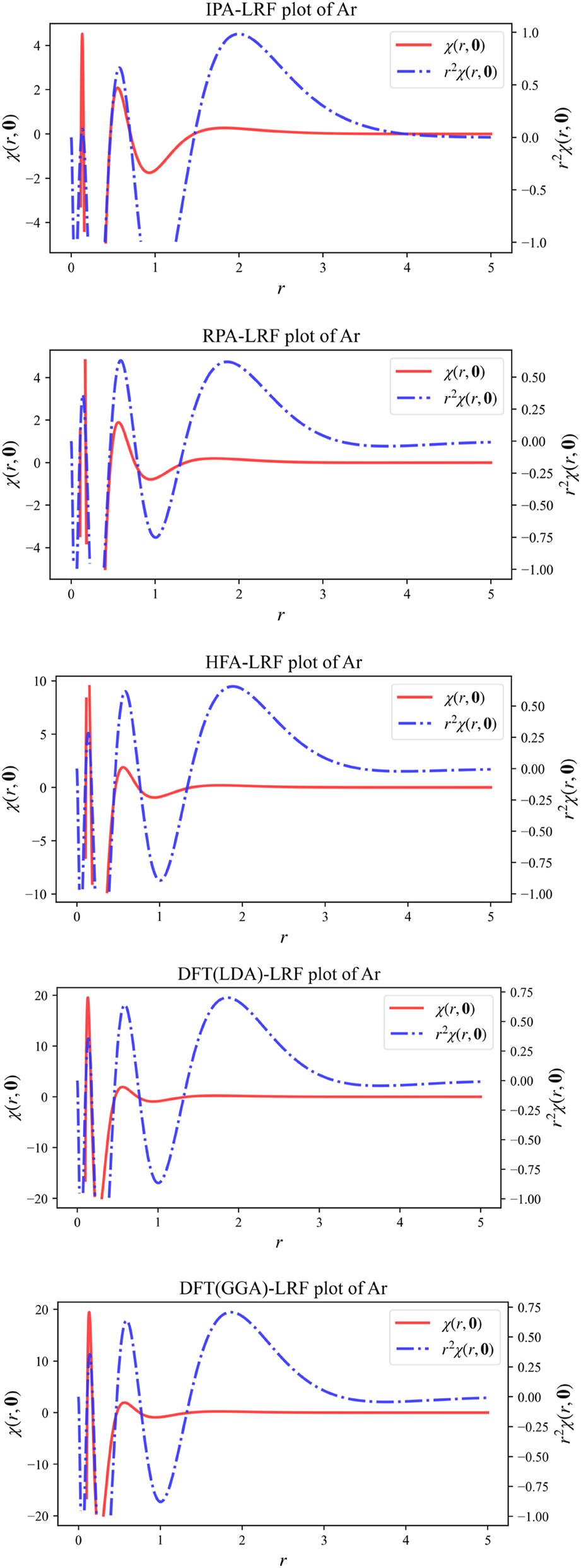
1D plots of χ(r,0) and r ² χ(r,0) for Ar, computed from B3LYP data using the IPA, HFA, RPA and DFT expressions, the latter computed both with the LDA and (full) GGA approximations for f _xc ( r , r ^′). Reprinted with permission from Wang, B.; Geerlings, P.; Van Alsenoy, C.; Heidar-Zadeh, F.; Ayers, P. W.; De Proft, F. J. Chem. Theor. Comp. 2023, 19, 3223–3236. Copyright 2023, American Chemical Society.

In 2D, r 2 r ′ 2 χ r , r ′ , defined as

(46) r 2 r ′ 2 χ r , r ′ = ∫ r 2 r ′ 2 χ r , r ′ sin θ d θ   d φ sin θ ′ d θ ′ d φ ′

will be plotted, obtained by integrating χ( r , r ^′) over all angular variables. These plots will show the density response “intensity” for a given region of the atom, depicting the density response at a distance r to perturbation at distance r’ obtained after spherically averaging.

Figure 3 depicts plots of the B3LYP radial distribution type expression of the LRF r 2 r ′ 2 χ r , r ′ at all levels of theory. Again, the overall structure of these plots is highly similar, giving confidence in the IPA results published previously and also given in this Figure, confirming that chemical insights can already be extracted at this level. As can be seen, these plots are symmetrical w.r.t. the diagonal due to the symmetry of the kernel χ( r , r ^′) = χ( r ^′, r ). The negative regions are mainly located along the diagonal in line with the negativity of the diagonal elements χ( r , r ). When compared to the 1D plots, the 2D plots provide a more detailed vision on the density/potential perturbation relation, showing for example oscillations for all r (or r’) values and not only for the r (or r’) = 0 case, thereby revealing more intricate consequences of the atomic shell structure.

Fig. 3:

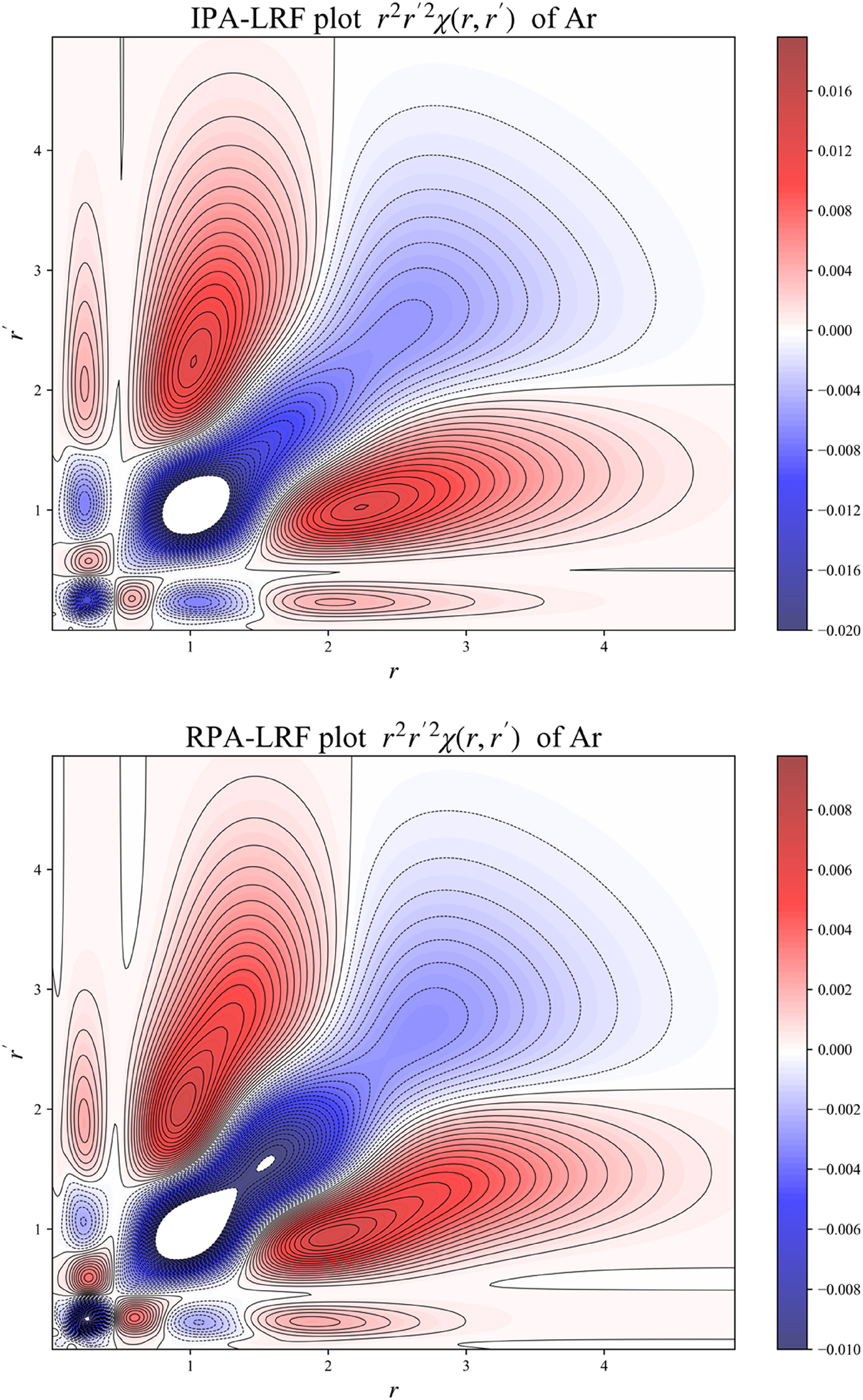
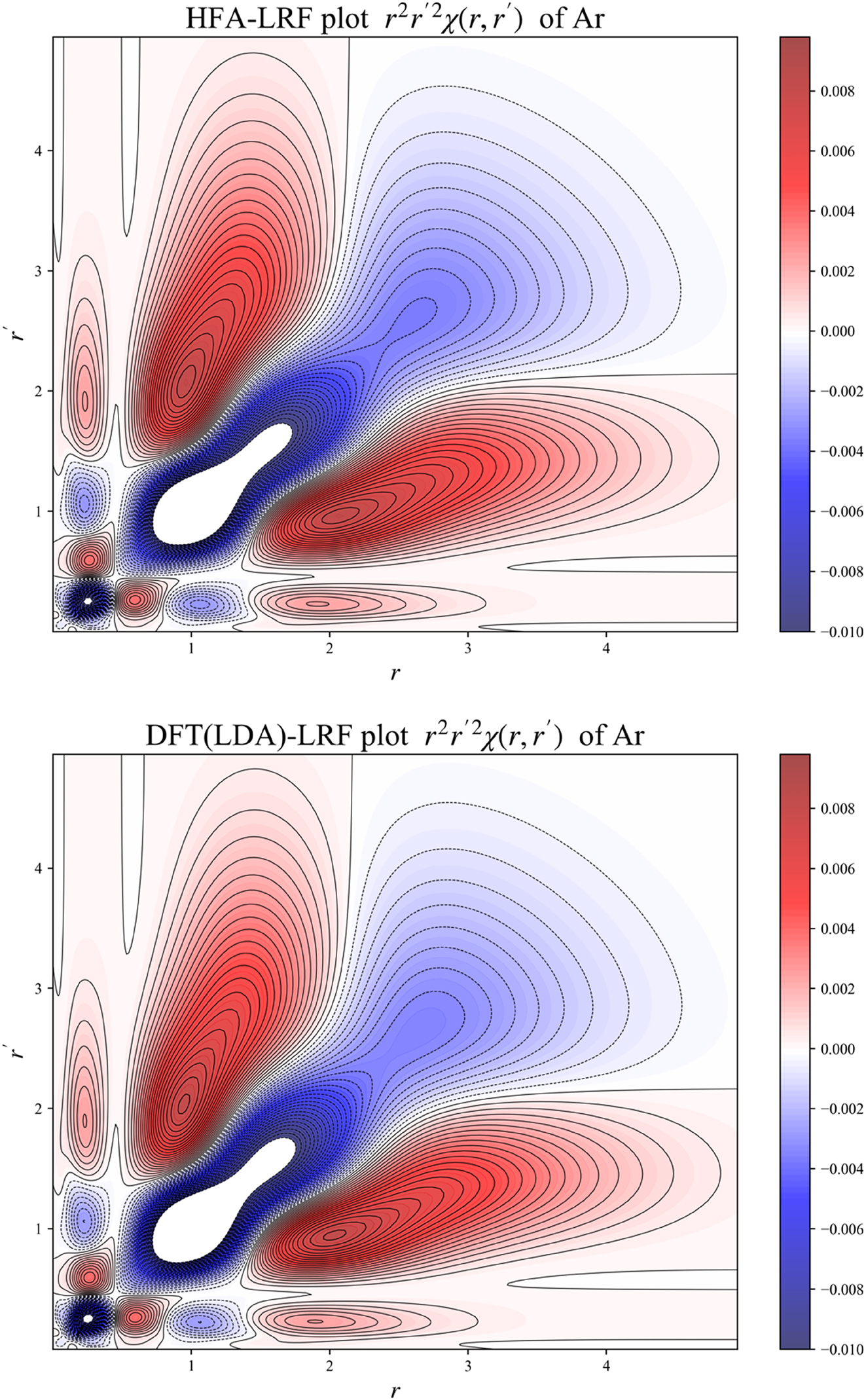
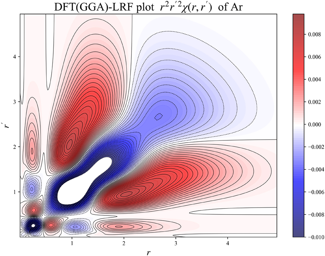
2D plot for r 2 r ′ 2 χ r , r ′ of the Ar atom, computed from B3LYP data, using the IPA, HFA, RPA and DFT expressions, the latter computed both with the LDA and (full) GGA approximations for f _xc ( r , r ^′). Reprinted with permission from Wang, B.; Geerlings, P.; Van Alsenoy, C.; Heidar-Zadeh, F.; Ayers, P. W.; De Proft, F. J. Chem. Theor. Comp. 2023, 19, 3223–3236. Copyright 2023, American Chemical Society.

The 3D representation, given again for the different approximations in Fig. 4 for the Ar atom, represents surface plots of χ( r ,0), showing the response of the density at position r with respect to a perturbation at the position of the nucleus with r ^′ = 0. r is placed in the XY plane with the nucleus centered at the origin. Again, the shell structure can be clearly observed and no large qualitative differences between the different approximations can be noticed.

Fig. 4:

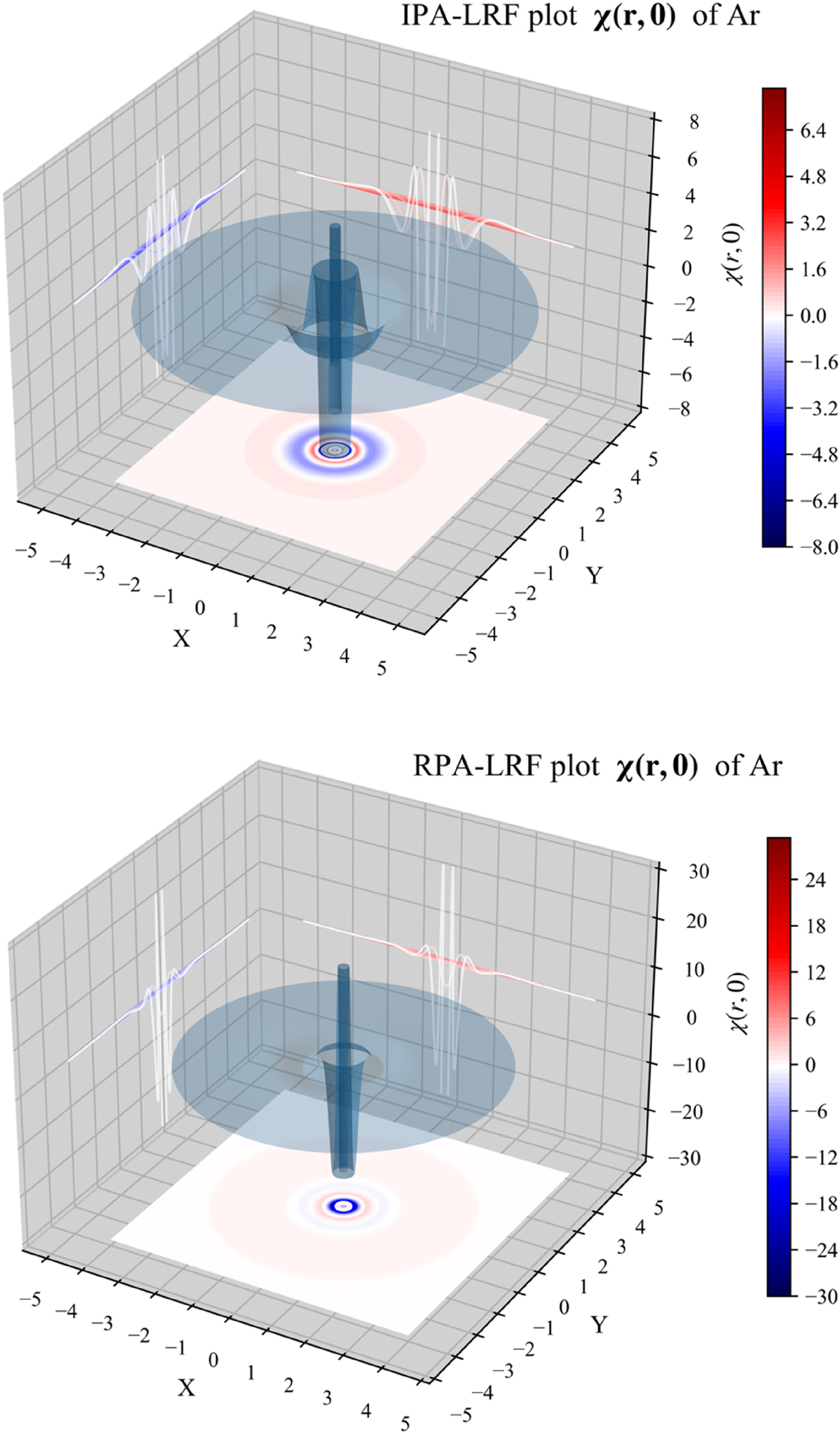
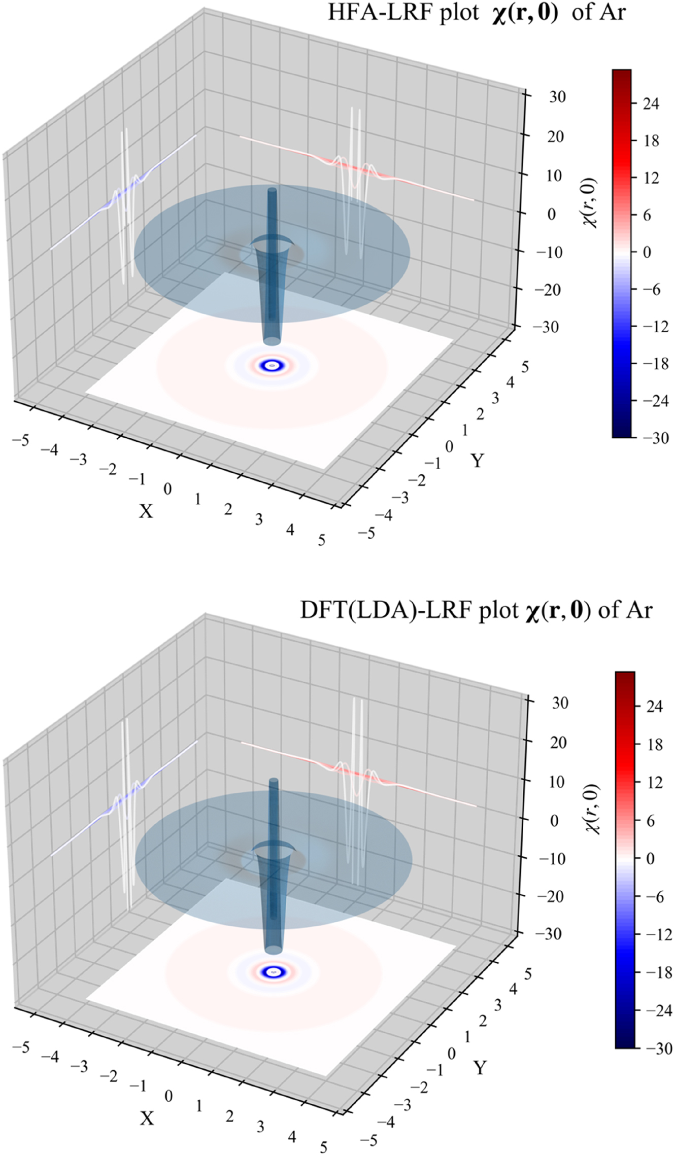
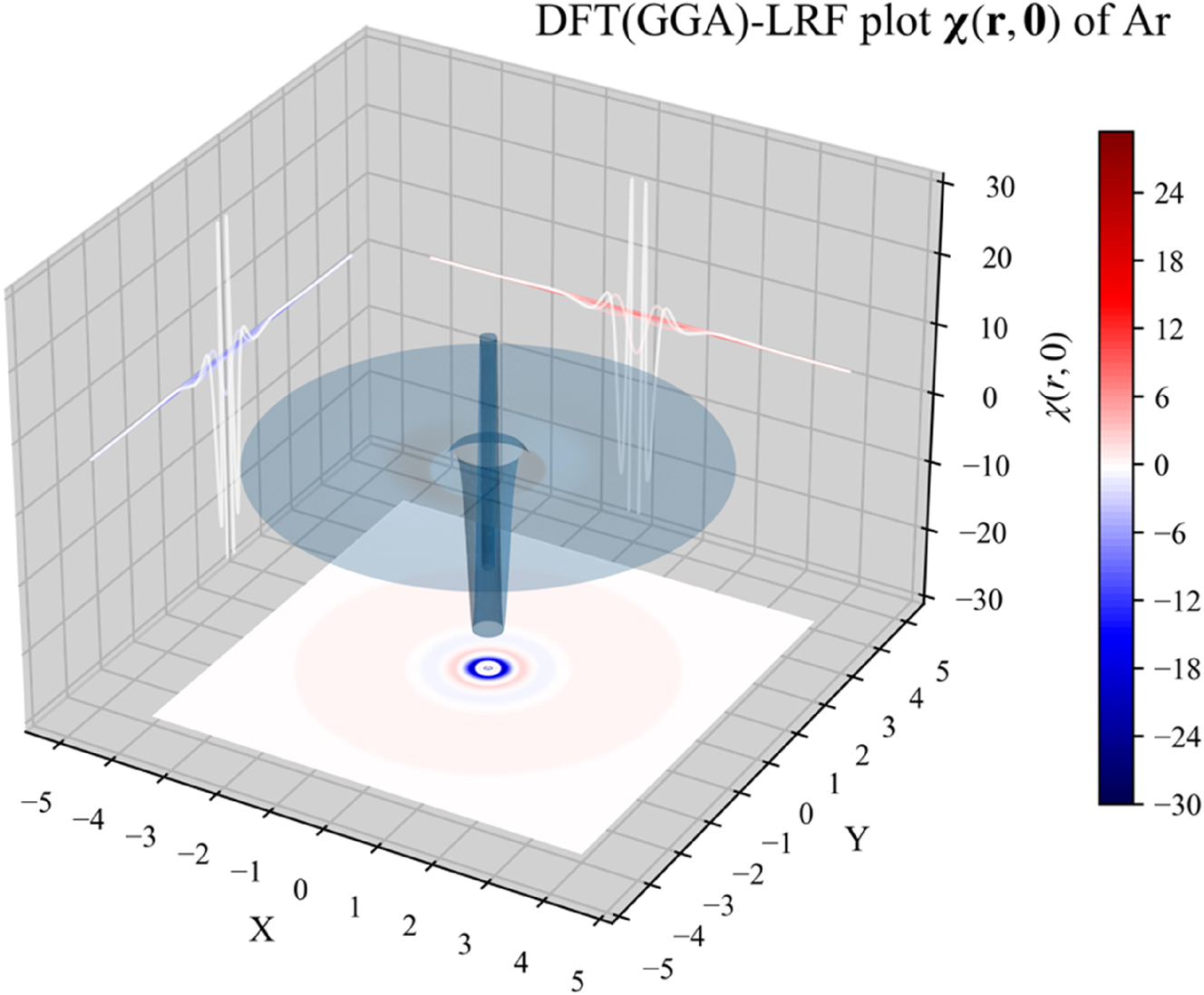
3D plot of χ( r ,0) for the Ar atom, computed from B3LYP data, using the IPA, HFA, RPA and DFT expressions, the latter computed both with the LDA and (full) GGA approximations for f _xc ( r , r ^′). Reprinted with permission from Wang, B.; Geerlings, P.; Van Alsenoy, C.; Heidar-Zadeh, F.; Ayers, P. W.; De Proft, F. J. Chem. Theor. Comp. 2023, 19, 3223–3236. Copyright 2023, American Chemical Society.

We finally focus specifically on the comparison of the simplest (LDA) and the most elaborate (GGA) level for the f _xc term in the linear response function plots in 1D, 2D and 3D to scrutinze explicitly the contribution of the gradient corrections. The difference between the LDA and GGA levels is negligibly small, implying that, for atoms, the LDA part of the kernel is the main contribution to the linear response function; one can thus anticipate that the difference between LDA and GGA levels, both in the uncondensed and condensed form, for molecules will be small. As a consequence, qualitative agreement can certainly be expected.

3.1.3 Molecules

In our previous work, the LRF was used to investigate inductive and mesomeric effects, delocalization and aromaticity. This was mainly done using the linear response matrix (CLRM), obtained as

(47) χ A B ≡ ∫ ∫ χ r , r ′ w A r w B r ′ d r d r ′ = − 4 ∑ i a , j b M − 1 i a , j b S i a A S j b B

The standard Hirshfeld atomic partitioning scheme was used to obtain the elements of this matrix.

The results will obviously depend on the fundamental level of theory (the DFA to calculate the Kohn Sham orbitals) but also on the level at which the LRF is evaluated (Eqs. (43)–(45)). The latter issue is of primary importance in this contribution and will now be discussed in detail. In Table 1 we compare, for a series of 10-electron molecules at a given DFA level (B3LYP), the different approximations for the off-diagonal elements of their atom condensed LRF matrix: IPA, RPA, HFA (for completeness), DFT(LDA) and DFT (GGA). DFT (LDA) refers to the inclusion of only the density-density term in the f _xc term in Eq. (45), DFT(GGA) to including also the mixed density/density gradient and the double density gradient terms. In Table 2, the contributions of the different terms in the f _xc term are further scrutinized.

Table 1:

Off-diagonal elements of the Atom-Condensed LRF matrix elements for 10-electron molecules, obtained from B3LYP orbitals and energy levels, at different levels of approximation (see text).

	IPA	RPA	HFA	DFT(LDA)	DFT(GGA)
HF	0.5644	0.2983	0.3725	0.3536	0.3768
H2O	0.5544	0.2517	0.3167	0.2998	0.3148
NH3	0.4913	0.2068	0.2634	0.2486	0.2582
CH4	0.3833	0.1603	0.2105	0.1988	0.2049

Table 2:

Comparison between different approximations to the f _xc kernel contribution for the off-diagonal element of the Atom-Condensed LRF, χ_AF (A = C, N, O, and F).^a

LRF	B3LYP (LDA)	B3LYP (LDA + GGA1)	B3LYP (LDA + GGA1+GGA2)	Correction % (GGA1→LDA)	Correction % (GGA2→LDA + GGA1)
HF	0.3536	0.3842	0.3768	8.65	−1.93
H2O	0.2998	0.3185	0.3148	6.24	−0.27
NH3	0.2486	0.2589	0.2582	4.14	−0.07
CH4	0.1988	0.2031	0.2049	2.16	0.18

1. ^aLDA, GGA¹ and GGA² stand for the local density (first term), density-gradient (second and third terms), and gradient-gradient (fourth term) contributions in Eq. (45), respectively.

Table 1 shows that an important difference in the actual values is to be noted when passing from IPA to RPA, appreciably larger than when passing from RPA to DFT (both at LDA and GGA levels). However, the trends between the four molecules are identical for all levels. Scrutinizing the f _xc contributions in Table 2, the GGA correction to the LDA term changes the LRF value of the density/density term (LDA) by less than 10 %. More precisely the average contribution from the mixed density/density gradient term amounts to 5.3 %, whereas the contribution from the gradient/gradient term is less than 1 %. Consequently, chemical trends are insensitive to these corrections. It is thus plausible to hypothesize that including higher order corrections involving the Laplacian of the density or the kinetic energy density will be even smaller.

Overall, it can be stated that the evolution of the level of theory for the evaluation of the LRF shows a smooth behavior. If one is interested only in qualitative aspects (trends) the IPA approximation already does well. If numerical accuracy (“numbers”) is aimed at, already trustworthy results can be obtained by restricting the f _xc contribution to the LDA level, be it that the full DFT expression is at the user’s disposal.

As a confirmation, we now present in Fig. 5 the condensed LRF values between C₁ to C₆ of aromatic and non-aromatic six membered rings (benzene, phenol, cyclohexane and cyclohexanol) at the IPA, RPA, and DFT levels, systems we originally studied at the IPA level. ⁷⁰ In this Figure, we plot the LRF χ c 1 − c n (with n = 2, 3, 4, 5, 6), representing the density response of the given carbon atoms when the potential perturbation is exerted on carbon atom 1. The blue and red colors represent the aromatic and non-aromatic systems respectively. As can be seen and as observed in our previous work, for aromatic molecules, high LRF values appear at ortho (C₂, C₆) and para (C₄) positions accentuating mesomerically active atoms. This behavior disappears for non-aromatic molecules and the LRF value decreases with increasing distance only reflecting inductive effects. As can be seen, these distinct “zigzag” and “decay” behaviors are observed for all approximations, illustrating that revealing the mesomeric and inductive effects are qualitatively trustworthy at the simplest (IPA) level. Quantitatively however, some differences can be noticed. The IPA has the highest value, while RPA, HFA and DFT have similar but much smaller values. Nevertheless, IPA is a qualitatively correct approximation for the condensed LRF consolidating our earlier work. However, to obtain quantitively trustworthy values, it is recommended to perform the calculation using the DFT “full” expression (from which, according to our work, the GGA correction in the exchange-correlation kernel is not necessary and can be left out).

Fig. 5:

Atom-condensed LRF for aromatic and nonaromatic 6-membered rings (C₁-C_n where n = 2, 3, 4, 5, 6) at the IPA, HFA, RPA and DFT levels of approximation. At the DFT level, the exchange-correlation kernel only includes the LDA part. Reprinted with permission from Wang, B.; Geerlings, P.; Van Alsenoy, C.; Heidar-Zadeh, F.; Ayers, P. W.; De Proft, F. J. Chem. Theor. Comp. 2023, 19, 3223–3236. Copyright 2023, American Chemical Society.

3.1.4 Conclusions

The studies presented in this section show that evaluation of a well-defined concept, the linear response function as the second derivative of the energy with respect to the external potential, could be refined “smoothly” to obtain better “numbers”, though gradually demanding more analytical and computational efforts, the qualitative aspects being however unchanged.

3.2 The Fukui function

In this section we will investigate whether the mixed second derivative of the energy with respect to the number of electrons N and the external potential v( r ), (δ ² E/∂Nδv( r )) termed the Fukui function f( r ) (see Section 2), shows the same behavior allowing a smooth refinement toward quantitatively more accurate numbers.

In Section 2 it was shown that this second derivative boils down to the partial derivative of the electron density ρ( r ) with respect to the number of electrons N at constant external potential (∂ρ( r )/∂N)_v which is the key expression discussed in the present section.

First of all, there is the analogy with the linear response function as both quantities are in fact more precise/general definitions of well-known concepts of the older literature. As stated above the LRF can be considered as an extension/generalization of Coulson’s atom-atom polarizability, ¹¹ launched in the context of the above mentioned Hückel approach to π-electron systems. ¹⁰ The Fukui function is a generalization of Fukui’s frontier orbital model, ⁴³ in which the molecular reactivity is described solely in terms of the frontier orbitals, the HOMO and the LUMO. Indeed, its definition shows that the N derivative pertains the complete electron density, involving all orbitals of the system.

After its launching in 1984 by Yang and Parr ⁴² the finite difference approach, as presented in the original paper, has become the default method in nearly all of the (numerous) evaluations of the Fukui function. ^{24 , 29} Taking the N derivative of the density, at a given reference N value, typically the neutral atom value, then occurs separately for the electron deficient and the electron abundant side. Considering the density values of the neutral, cationic and anionic systems the standard finite difference approach then leads to the well-known expressions for the left and right Fukui functions, f ⁻ (r) and f ⁺ (r) (where N should be regarded as the reference value; cf. Eqs. (26) and (27))

(48) f F D − r = ρ N r − ρ N − 1 r

(49) f F D + r = ρ N + 1 r − ρ N r

In the frozen core approximation, it is easily seen that these expressions reduce to the HOMO and LUMO densities, respectively, regaining Fukui’s frontier orbital approach ^{21 , 42}

(50) f F O − r = ρ HOMO r

(51) f F O + r = ρ LUMO r

The finite difference approximation however presents two disadvantages: separate calculations for the neutral and charged systems are necessary, and in the case of f ⁺one is forced to consider the anion of the system which is very often unstable necessitating a number of approximate schemes to avoid the negative electron affinity problem. ^{21 , 76 , 77 , 78 , 79 , 80} The solution to the problem in order to get better “numbers” was refining the evaluation and passing to an analytical evaluation of the Fukui function. The derivation was presented in a joint effort with Yang and Cohen, ⁸¹ using (cf. Section 3.1) a Coupled Perturbed Kohn Sham ^{82 , 83 , 84} approach. The tricky derivative with respect to N was thereby circumvented by starting from the alternative expression for the Fukui function as the functional derivative of the electronic chemical potential μ with respect to the external potential at constant N, (δμ/δv( r ))_N, related by a Maxwell relation to the one presented above. The following equations were obtained for closed shell systems where here the case of Kohn–Sham DFT is selected with f referring to a frontier orbital, HOMO or LUMO.

(52) ∂ 2 E ∂ N δ v r = f r = φ f r 2 − ∑ i a , j b M − 1 i a , j b K f f , i a f f φ j r φ b r

The M matrix of Section 3.1 reappears in view of the CPKS ansatz and the K i a f f matrix is defined in the Kohn Sham DFT case as

(53) K f f , i a f f = 4 f f | i a + 4 f f | f x c r , r ′ i a

Depending on the nature of the DFA functional, varying from pure DFT functionals (LDA, GGA, …) to hybrid and range separated functionals on the Jacob’s ladder ⁴⁷ (with modifications of the f _xc integral if exact exchange is present as in Section 3.1) the explicit form of the equations changes, as in Section 3.1 for the LRF. In the same vein the equations for the Hartree Fock case can easily be written down. Eq (52) is an analytical proof that the exact Fukui function can be seen as the sum of a frontier orbital density and a correction term, thereby retrieving 1° the frozen orbital expressions in Eqs. (50) and (51) as a first order approximation and 2° Parr and Pucci’s earlier alternative approach to an exact Fukui function (Section 2, ⁵⁶ ) where the correction term involves orbital N-derivatives. Intuitively, recognizing the importance of the frontier orbitals in Fukui’s reactivity theory, the correction can be expected to be relatively small.

Though a few examples of the analytical approach were already presented in Ref. 81] only recently a detailed and comprehensive comparison between the finite difference and analytical approaches was presented. We here select from that study the case of substituted benzenes, for which the evaluation of the Fukui functions, especially f ⁻, has been at stake since the early days of conceptual DFT. ⁸⁵ The ultimate aim thereby was to investigate the capability of the Fukui function in predicting the ortho, meta, para selectivity upon electrophilic aromatic substitutions. In Fig. 6 we show the comparison between the analytical and finite difference atom condensed Fukui functions for benzene and a number of substituted benzenes with substituents displaying both electron donor and electron acceptor properties (–O⁻, –NH₂, –OH, –OCH₃, –SH, –CHCH₂, –CH₃, –Br, –Cl, –F, –COOH, –CHO, –CN, and –NO₂). The condensed Fukui functions were obtained as (cf. Eqs. (30) and (31))

(54) f A − = q N − 1 A − q N A

(55) f A + = q N A − q N + 1 A

where q indicates the charge on atom A in the N, N-1 and N+1 electron system, respectively. In the case of benzene itself the finite difference calculations were run with a doubly charged cation and anion (dividing the result by a factor 2) to avoid symmetry breaking due to the presence of a doubly degenerate HOMO and LUMO. All calculations refer to a PBE/cc-PVTZ level of theory ⁸⁶ with Hirshfeld type techniques ⁸⁷ for atomic condensations.

Fig. 6:

Linear correlation between Fukui functions (a) f ⁻ and (b) f ⁺ calculated by both the analytical and finite difference approach for benzene with different substituents at ortho, meta and para positions; outliers are highlighted (see text). Reprinted with permission from Wang, B.; Geerlings, P.; Liu, S. B.; De Proft, F. J. Chem. Theor. Comp. 2024, 20, 1169–1184. Copyright 2024, American Chemical Society.

Figure 6 shows that when leaving out the outliers (vide infra) fair correlations with R² = 0.970 and 0.920 for f ⁻ and f ⁺ respectively are found. The intercept is small and the linear term in the regression equations shows that the analytical and finite difference Fukui functions differ by about 10 %, a relatively small factor. The O⁻ substituent in case of f ⁺ is clearly an outlier, due to the inappropriate treatment of the double anion in the finite difference calculation, revealing an obvious shortcoming of the finite difference method. Remarkably for f ⁺ the inductive and mesomeric electron withdrawing (-M, -I) groups –CHO, –COOH and –NO₂ are also outliers. Their disagreement can be traced back to a fundamental issue in the E vs. N curves: in standard applications of CDFT Parr’s parabolic approach ²¹ is adopted ^{24 , 29} (Section 2) based on energy values at integer N values. Over the years this approach led to a variety of results which are mostly in agreement with “chemical” intuition, for example linking the electronic chemical potential and the hardness to the average and the difference between ionization energy and electron affinity, respectively (see Section 2). However, digging deeper in the E vs. N behavior and including fractional electron numbers, a more refined picture appears, dictating a series-of-intersecting-straight-lines behavior in the case of the exact exchange correlation functional. ⁵⁰ This behavior is represented by the following equation

(56) E N + λ = 1 − λ E N + λ E N + 1 ,

expressing that the energy at fractional electron number N+λ with 0 < λ < 1 is a linear combination of the N and N+1 energies. This behavior is at the origin of the N derivative discontinuity of the μ vs. N curve at integer N ⁵⁰ that will be at stake in Section (3.3). For most of the DFAs the E(N) curve however displays a piecewise convex behavior, in the Hartree–Fock case a piecewise concave behavior (Fig. 7). ^{88 , 89 , 90}

Fig. 7:

The E vs N curve and its consequences for the analytical evaluation of CDFT response functions. (a) schematic E vs N curves for the exact functional, most DFAs and the Hartree–Fock method indicating piecewise-linear, -convex and -concave behavior respectively (b) analytical conceptual DFT “stairs” under 0K limit, blue and orange regions indicating zero and first order N-derivatives, and white blocks are second or higher order N-derivatives whose analytical evaluation is hampered by the derivative discontinuity. (see text). Reprinted with permission from Wang, B.; Geerlings, P.; Liu, S. B.; De Proft, F. J. Chem. Theor. Comp. 2024, 20, 1169–1184. Copyright 2024, American Chemical Society.

As the density is the functional derivate of the energy with respect to the external potential (Section 2) an analogous behavior for the ρ( r ) vs. N curve can be expected, ⁹¹ with only a linear piecewise behavior for the exact density which can be written as

(57) ρ N + λ r = 1 − λ ρ N r + λ ρ N + 1 r

The deviations from piecewise linearity in the E = E(N), and consequently for the density curve, are ascribed to the delocalization error (DE), affecting the DFAs, which itself originates from the self-interaction error (SIE). ^{92 , 93 , 94}

The dependence of the chosen frontier orbital f of the analytical expression in Eq. (52) retrieves the difference in the left/right derivative of ρ( r ) at a single integer N, in according with the derivative discontinuity at integer N. The finite difference approach manipulates slopes involving two ρ values pertaining integer N and N+1.

A more concrete picture is given in Fig. 8 where the behavior of the charges at ortho, meta and para positions with small fractional occupation number (up to +/− 0.01) is given for four substituted benzene systems: –OH, –CHO, –CN and –NO₂. The arrow at fractional charge zero points to the out-of-range integer charge values for the cation and anion, calculated with integer occupation.

Fig. 8:

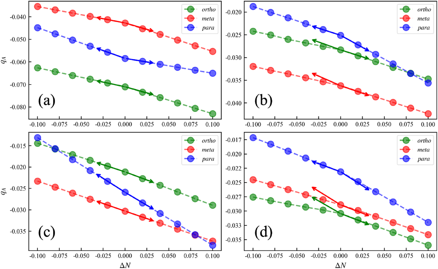
Behavior of Hirshfeld charge at ortho, meta and para position with small fractional occupation number (up to +/−0.01; dashed line) for substituted benzene systems: (a) –OH, (b) –CHO, (c) –CN and (d) –NO₂. The arrows point to the out-of-range cation and anion values calculated with integer occupation. Reprinted with permission from Wang, B.; Geerlings, P.; Liu, S. B.; De Proft, F. J. Chem. Theor. Comp. 2024, 20, 1169–1184. Copyright 2024, American Chemical Society.

For well-behaved systems, Fig. 8a and c, the linearity obtained from fractional occupation is in line with the finite difference method, which indicates that the ρ vs. N curve is indeed (approximately) piece-wise linear (Eq. (57)) in these cases; as a result their finite difference and analytical Fukui functions are similar. In Fig. 8b and d, however, the dashed line is below the solid arrow thus yielding a convex behavior for the ρ vs. N curve similar to the E vs. N curve, obtained with fractional occupation numbers, which causes the difference between the two approaches in calculating the Fukui function. According to Eq. (52) the Fukui function can be written as the difference between the frontier orbital density, and a second term, involving all orbitals, occupied and unoccupied. This situation was already implicitly put forward in the above-mentioned alternative approach by Yang, Parr and Pucci, ⁵⁶ writing the Fukui function as a frontier orbital density term corrected by a term involving N-derivatives of the orbitals. Since in practice the frontier orbital density term is usually much larger in value than the second one, the overall result might indicate that the Fukui function might be less sensitive to the delocalization error than the hardness which will be treated in the next section.

So, how to choose between the analytical and finite difference method in chemical reactivity studies?

Let us start from the fact that when the exact (but unknown) functional is used both the finite difference and the analytical method should give the same results due to what we can call the Fukui function “condition” which should be obeyed in that exact case

(58) f N + λ r = ρ N + 1 r − ρ N r

(the term “condition” ^{81 , 95} will be explained in more detail in the next section). If the (approximate by default) DFA can give highly accurate densities for neutral and charged states the finite difference approach for f ⁻ may then be preferable for practical reasons, though requiring two calculations. The evaluation of f ⁺ involving negatively charged systems is however expected to be not trustworthy in many cases in the finite difference approximation which is not the case for the analytical evaluation for which anyway DFAs with minor (de)localization error are needed. So, the rule of thumb for the Fukui function evaluation: the analytical approach should be by far preferred for the study of negatively charged systems whereas the finite difference approach might be more reliable for f ⁺ in case of too much delocalization error.

In conclusion, this section leads to a result on “numbers for concepts” which differs from that in Section 3.1. Here, refinement, i.e. the analytical evaluation instead of the finite difference approximation, not always leads to better “numbers” contrasting with the conclusions of Section 3.1. The reason is that deep lying fundamental aspects of the underlying physics, the nature of the E vs. N curve, come into play in this mixed N and v derivative which were not at stake in the refinement of the Linear Response Function which is a pure v-derivative. In our view the Fukui function case can be considered as an example of what Löwdin ⁹⁶ once described in more general terms on what happens when refining a theory as depicted in Fig. 9. Starting from simple concepts one reaches at a certain level of sophistication an almost perfect agreement between theory and experiment. Upon further improving the theory the agreement gets worse and worse, reaching a minimum, but from that point on the curve rises again and (hopefully) in the asymptotic limit approaches perfect agreement between theory and experiment. The two particular points were termed by Löwdin as the “Pauling point” and the “PhD point” respectively.

Fig. 9:

Löwdin’s diagram; agreement between theory and experiment vs. refinement of the theory (re-drawn after P.O. Löwdin, International Journal of Quantum Chemistry: Quantum Chemistry Symposium 1986, 19, 19–37). ⁹⁶

Roughly speaking one could, in analogy, consider that in our endeavor of refining the Fukui function results in order to get better “numbers”, the Pauling point refers to the finite difference approximation with moderate DFAs, and that the further refinement by taking analytical derivatives is only partial successful due to the underlying characteristics of the E = E(N) curve caused by the delocalization error. Finally, however, upon increasing quality of the DFAs, the analytical method will yield results closer and closer to the exact result corresponding to the piecewise linear behavior.

3.3 The chemical hardness

As the third case in this Section we consider the second order E vs. N derivative, the chemical hardness η. In nearly all of the applied Conceptual DFT literature the hardness is evaluated starting from Eq. (22) in Section 2, resulting from Parr’s parabolic approach. The hardness is given by (half of) the difference between the ionization energy and the electron affinity of the (mostly neutral) system under consideration, ^{21 , 24} reducing to the “HOMO-LUMO gap” sometimes simply called “the gap” in a Koopmans’ type approximation (Eq. (23)). Note that we gradually pass from a pure v second derivative, the linear response function, to a mixed v and N one, the Fukui function, to a pure N second derivative. The appearance of a first N derivative in the previous subsection 3.2 already prompted us to a more thoughtful handling upon refinement to get better “numbers” as compared to the pure v second derivative. So what about this case if we, as in the two previous cases, refine the evaluation for the hardness through an analytical approach?

We here follow the derivation, originally proposed by Yang, Cohen and the present authors ⁸¹ and later on refined in our recent contribution, ³⁸ where from the start, and as opposed to the Parr expression, a left and right analytical hardness, η ⁻ and η ⁺ is imposed. The reason is the derivative discontinuity of the electronic chemical potential μ, in analogy with the derivative discontinuity of the density ρ( r ), giving rise to two Fukui functions f ⁻(r) and f ⁺(r) (vide supra).

The analytical hardness ∂ 2 E ∂ N 2 v r ± can then be evaluated as the derivative of the chemical potential μ i.e., the HOMO/LUMO energy ε _f with respect to the number of electrons, ^{97 , 98} as

(59) ∂ μ ∂ N v r ± = ∂ ε f ∂ N v r = f ∂ v J ∂ N + ∂ v x c ∂ N + α ∂ v k ∂ N f

where v _J , v _xc and v _k are the Coulomb potential, the exchange-correlation potential, and the Hartree–Fock exchange operator (cf. Section 3.1); v _xc is adapted to the fraction of Hartree–Fock exchange, α, used. For pure DFAs, where there is no contribution from exact exchange, Eq. (59) becomes

(60) η ± = f ∂ v J ∂ N + ∂ v x c ∂ N f = f ∂ ρ r ′ ∂ N δ v J δ ρ r ′ + δ v x c δ ρ r ′ f

which simplifies to Ref. 38], [81]

(61) η ± = K f f , f f η − ∑ i a , j b M − 1 i a , j b K f f , i a f f K f f , j b η

For closed shell systems, the M matrix is defined as in Section 3.2 whereas the K matrix elements are given by

(62) K f f , i a f f = 4 f f | i a + 4 f f | f x c r , r ′ i a

(63) K f f , f f η = f f | f f + f f | f x c r , r ′ f f

(64) K f f , j b η = f f | j b + f f | f x c r , r ′ j b

For hybrid functionals the nonlocal part of the exact exchange should also be taken into account. Since the Hartree–Fock exchange potential depends on the density matrix P( r , r ^′) as ²¹

(65) v k r , r ′ = − 1 2 P r ′ , r r ′ − r

with P( r ^′, r ) = P( r , r ^′), its contribution to the analytical hardness can be derived as

f ∂ v k P ∂ N f = 1 2 f r 1 ∫ δ v k P r 1 , r 1 ′ δ P r 2 , r 2 ′ ∂ P r 2 , r 2 ′ ∂ N d r 2 d r 2 ′ f r 1 ′ = − f r 1 1 r 1 − r 1 ′ f r 1 ′ , r 1 f r 1 ′

= − f r 1 1 r 1 − r 1 ′ ∑ p q F p q p r 1 ′ q r 1 f r 1 ′

(66) = − ∑ p q F p q f f | p q = − ∑ p q F p q f p | f q

where f( r , r ′) is the spatial Fukui matrix defined as the N derivative of the density matrix P(r,r′) and F _pq is the Fukui matrix in the MO basis, which is defined as the derivative of the MO density matrix (i.e., occupation number) with respect to the number of electrons, adding the corresponding orbital relaxation terms. ^{99 , 100} Written in terms of spatial coordinates, the Fukui matrix is

(67) f r , r ′ = ∑ p q F p q φ p r φ q r ′

or, more directly,

(68) f r , r ′ = φ f r φ f r ′ − ∑ i a , j b M − 1 i a , j b K f f , i a f f φ j r φ b r ′ + φ j r ′ φ b r / 2

Full mathematical details on the Fukui matrix and its properties can be found in a recent contribution. ⁴⁰

Using this formalism, the analytical hardness for hybrid functionals is

(69) η ± = K f f , f f η − ∑ i a , j b M − 1 i a , j b K f f , i a f f K f f , j b η − α ∑ p q F p q f p | f q

where the new M i a , j b and K f f , i a f f matrices contain an additional exchange part written as K i a , j b = i b | j a + i j | a b and K f i , f a = f i | f a respectively.

(70) M i a , j b = ε a − ε i δ i j δ a b + 4 i a | j b + 4 i a | f x c r , r ′ ; α j b − α K i a , j b

(71) K f f , i a f f = 4 f f | i a + 4 f f | f x c r , r ′ ; α i a − 2 α K f i , f a

The case of range-separated functionals, though more complicated (analogous to the case of the linear response function in Section 3.1), can be treated in a similar way and we refer to the original publication for the derivation and complete expression.

Using this apparatus the hardness can now analytically be evaluated for a broad series of DFAs. Figure 10 gives a broad overview of the analytical hardness values for H₂O for 35 DFAs varying from LDA to GGA to GGA, hybrids and the Coulomb attenuated CAM-B3LYP functional. First of all we remark that the analytical hardness η ^± is positive for DFAs and negative for Hartree–Fock, as expected, due to their delocalization and localization errors, respectively. ⁹⁰ For DFAs, the analytical hardness on the electron deficient side, η ⁻, is almost always 2 to 3 times bigger than on the electron abundant side. Since exact exchange numerically turns out to be negative (cf. Eq. (69)), larger α values give smaller analytical hardness. ⁹⁰

Fig. 10:

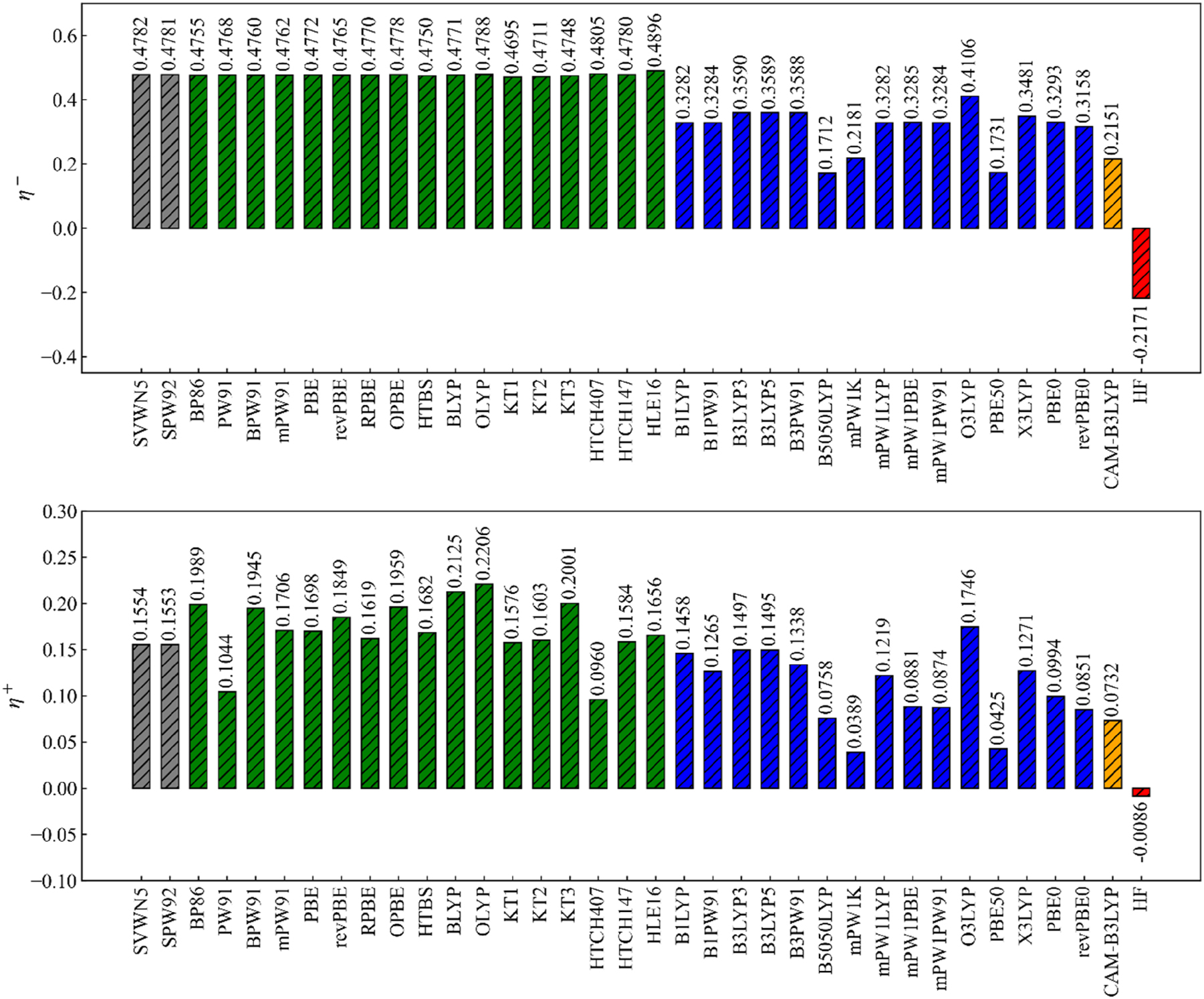
Bar chart of analytical hardness η ^± computed with various density functionals for H₂O. LDA, GGA, hybrid and range-separated functionals and HF are represented by grey, green, blue, orange and red color, respectively. Reprinted with permission from Wang, B.; Geerlings, P.; Heidar-Zadeh, F.; Ayers, P. W.; De Proft, F. J. Phys. Chem. Lett. 2024, 15, 11259–11267. Copyright 2024, American Chemical Society.

It is tempting to compare these values with the traditional Parr Pearson value obtained as I-A but a word of caution should be inserted at this moment. Upon refining the hardness evaluation by taking analytical second derivatives of E with respect to N we are in fact facing a fundamental problem, namely the piecewise linearity of the E vs. N curve, which could be coped with for the Fukui function, but which now becomes very problematic. As the first order derivative of E with respect to N,μ, gives a step function (vide supra) the second order derivative η should be zero on both sides: the derivative discontinuity problem. This leads to an unpleasant result because at first sight the hardness concept is threatened to disappear from the Conceptual DFT picture, where in the Parr-Pearson definition/expression it has gained widespread use and has been extremely useful in various domains of chemistry, thereby often bridging the theoretician’s and experimentalist’s worlds. ^{21 – 30} Its importance can hardly be overestimated. It should however be remembered that the definition was formulated in a quadratic approach to the E = E(N) curve, which does not display a derivative discontinuity, but which apparently resists to a refinement in terms of the intersecting straight lines model. From a chemist’s point of view, it is therefore unthinkable to discard this venerable approach (see also Ref. 29] for a recent discussion)

What to do? Two things: conserve the chemical content of the Parr-Pearson original definition and, on the other hand, exploit our findings on the “analytical hardness”, both its expression and numerical results. The solution should also be casted in a broader context by observing that, in analogy to the hardness, all response properties including second or higher order derivatives of N will in fact become zero for non-integer number of electrons N±λ for the exact functional at 0K and are ill defined at integer values N, as illustrated in Scheme 7b.

Concerning the chemical part we refer to Yang et al. who pointed out that a simple way out is to use the fundamental gap, defined as I-A or, equivalently the HOMO-LUMO gap, as the hardness1 ¹⁰¹ which aligns with Eqs. (22) and (23). Employing the I-A value (resulting from a quadratic E = E(N) curve) or the HOMO-LUMO gap is a sounder and chemically more meaningful candidate for chemical hardness than the η ^± values, which, we repeat, in the case of increasing quality of the v_xc should go to zero. The same strategy can also be used to obtain higher order N-derivatives, for example the hyper hardness γ = ∂ 3 E / ∂ N 3 v yielding γ = ε _LUMO-2 - ε _HOMO+ε _HOMO-1, or mixed second order N-derivatives such as the dual descriptor.

Another, but much more involved, way of addressing the derivative discontinuity, is to include temperature in the energy functional E[N,v( r ),T] and a lot of efforts in this field have been made by Ayers et al. ^{102 , 103 , 104 , 105 , 106} The E vs. N curve is smoothened by a not necessarily small temperature perturbation making it differentiable at the point N. In such way all response quantities are physically meaningful in theory but need to account for the temperature to which the system is exposed.

Is the refinement procedure and the expression/ values we obtained then in vain? On the contrary. As the values for the analytical hardness should be zero both at the electron deficient and abundant sides for the exact energy functional one can impose

(72) η + / − = 0

as (a) hardness condition(s), extended to higher orders ⁹⁵ including second or third order N derivatives, like the dual descriptor ^{60 , 61} and the hyper-hardness. ¹⁰⁷ The actual values are then a measure to estimate how much DFAs might differ from the exact functional due to the delocalization error. In other words, these values are a (be it non-unique) measure of the “quality” of the different DFAs.

Knowing this, we now re-interpret Fig. 10 in terms of the hardness condition. Starting with η ⁻, remarkably no significant improvement (i.e. lower value) can be observed in the pure DFAs when passing from LDA to GGA (and most probably meta-GGAs). A substantial decrease in the delocalization error is however observed for the hybrid functionals, with larger fractions of exact exchange giving rise to lower η ⁻ values. This is in line with the negative contribution of exact exchange to the analytical hardness (cf. Eq (69)). So larger α values give smaller analytical hardness ⁹⁰ and it then bears no surprise that PBE50 violates the hardness condition least. It is easy to obtain the order of magnitude of this improvement by using a weighted expression for the analytical hardness values

(73) η H Y B = 1 − α η G G A + α η H F

Using a η ^GGA = 0.48 and η ^GGA = −0.22 for HF, one obtains η ^HYB = 0.31 for a hybrid functional with 25 % exact exchange, in line with the numerical data in Ref. 39]. Range-separated functionals show further improvement, which can be traced back, presumably, to the large fraction of long-range exact exchange in these functionals. Finally note the (only) negative value for Hartree Fock in line with its piecewise concave behavior, as anticipated.

Overall, the hardness condition on the electron abundant side η ⁺ shows similar behavior as η ⁻ though somewhat more fluctuating.

Digging further in the positive aspects of the refinement procedure we refer to Ref. 89] where Hait and Head-Gordon assess the delocalization error in frequently used DFAs by inserting a linear delocalization function, which we denote as g(x) with g(x) = ax + b, into the energy’s piecewise linearity condition yielding.

E N − x = E N + x g x E N − 1 − E N

(74) ≈ E N + x a x + b E N − 1 − E N

(Ensuring that g(1) = 1 requires b = 1−a) They then fit g(x) to the energy values from fractional occupation calculations for various DFAs. Taking H₂O as an example, it is shown that a linear delocalization function fits E(N) well for most DFAs suggesting that the quadratic coefficient a could be a measure of the (de)localization error. So a relationship between η^+/−and a could be foreshadowed. Figure 11 indeed shows that there is an almost perfect linear correlation between Hait and Gordons a value and our computed values for (in this case) η⁻. This relationship can be justified by taking the second derivative of Eq. (74) with respect to the number of electrons N yielding

(75) η − ≡ η N − x ≈ 2 a E N − 1 − E N

Fig. 11:

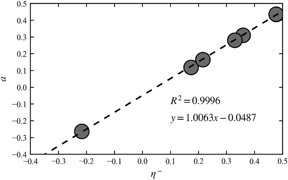
Linear correlation between the analytical hardness η ⁻ (Eq. (69)) for H₂O and the fitted parameter a for BLYP, PBE, B3LYP3, PBE0, PBE50, CAM-B3LYP and HF. Reprinted with permission from Wang, B.; Geerlings, P.; Heidar-Zadeh, F.; Ayers, P. W.; De Proft, F. J. Phys. Chem. Lett. 2024, 15, 11259–11267. Copyright 2024, American Chemical Society.

The analytical hardness thus turns out to be a linear function of the parameter a and the ionization energy (IE). Our numerical results in Ref. 39] lead to η ⁻≈0.9092a with a slope which is also very close to 1.

Though highly useful, Eq. (74) shows a dependence on the ionization energy (and in case of η⁺ on the electron affinity) necessitating the evaluation of the energy of both the neutral and a singly charged system. This calls for two calculations, which is sometimes problematic when anionic states are involved (vide supra). A way out is the following. Ref. 89] shows that the area between the real g(x) = ax + b and the ideal g(x) = 1 curve is |a|/2 and the area between Eq. (56) (when rewritten in terms of x) and Eq. (74) is |a|(E(N-1)-E(N))/6. Inserting Eq. (75) into the latter, the area reflecting the error for the energy curve, denoted as A, boils down to

(76) A = 1 12 η −

without explicit dependence on the ionization energy, or in case η ⁻ in the electron affinity. An explicit and simple expression thereby appears characterizing the delocalization error only in terms of the analytical hardness. The advantage of consideringη ⁻ orη ⁺is of course that the A value can be obtained from a single SCF calculation rather than a series of nonstandard DFT calculations with fractional occupations. Besides its diagnostic value this approach also yields an explicit expression of the energy curve for fractional occupation x in a quadratic approximation, as easily seen by inserting (75) into (74)

(77) E N − x = E N + I − 1 2 η − x + 1 2 η − x 2

where the contribution of the ionization energy can no longer be omitted. This equation was used to evaluate the E versus N curve using for PBE, CAM-B3LYP, PBE50 ^{75 , 86 , 108} and HF where the E(N) value has been set to zero. The areas A are also shown for PBE and PBE50. The three DFAs show, as expected, a convex behaviour, with larger delocalization error associated with greater analytical hardness. The curve of the HF method shown for comparison displays the expected concave pattern. In terms of the area between the exact and approximate energy curve, Eq. (76), Fig. 12 shows the area for both the PBE and PBE50 curves. The area for PBE (η ⁻ = 0.4772) is much larger than that of PBE50 (η ⁻ = 0.1731), in agreement with Eq. (76). Figure 12 indicates that it is feasible to predict the energy curve from a single SCF calculation; it is not necessary to converge SCF calculations for multiple fractional occupations.

Fig. 12:

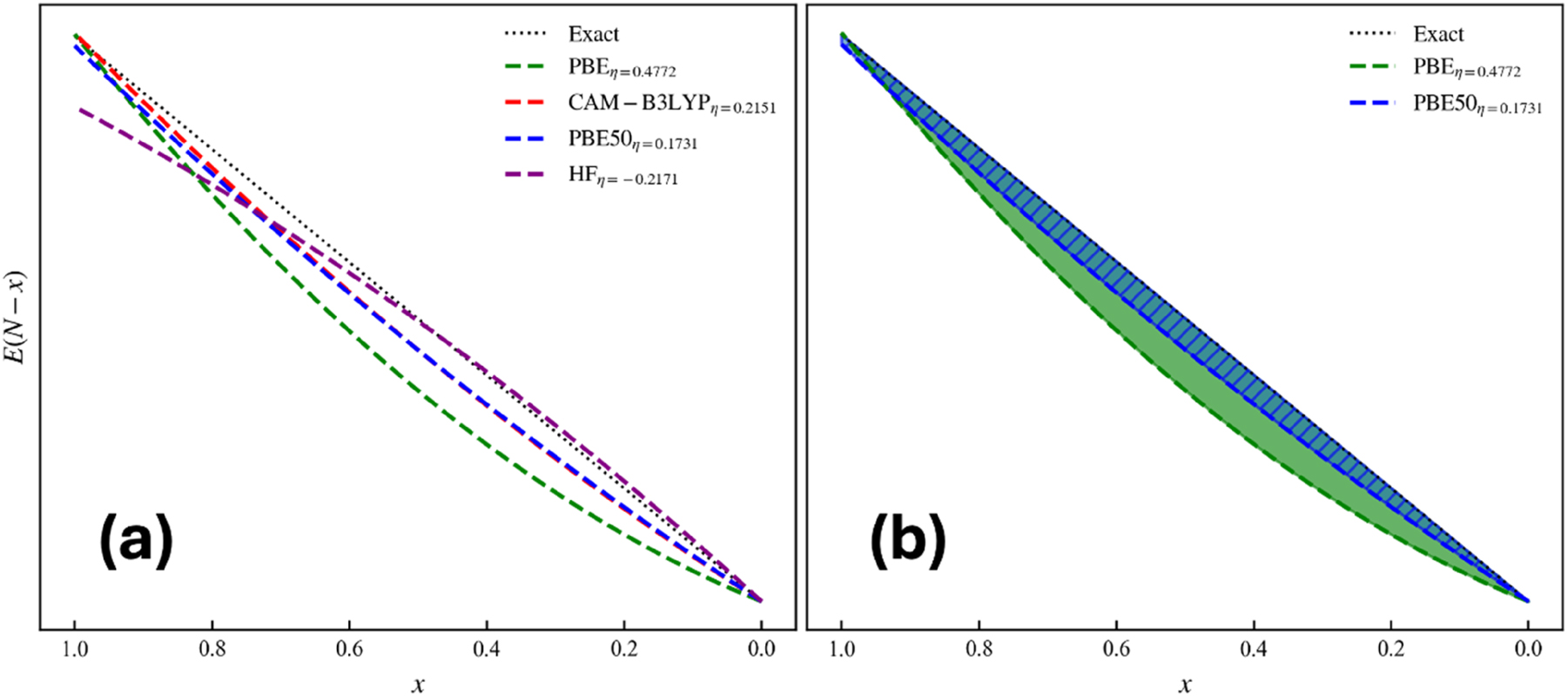
Evaluating the E vs. N curve. (a) The E versus N curve for fractional charge x calculated from Eq. (77) with the neutral reference E(N) set to the same value for all functionals (exact referring to the experimental IE) and (b) filled areas between the exact curve and the PBE (solid green) and PBE50 (blue line) functionals. Reprinted with permission from Wang, B.; Geerlings, P.; Heidar-Zadeh, F.; Ayers, P. W.; De Proft, F. J. Phys. Chem. Lett. 2024, 15, 11259–11267. Copyright 2024, American Chemical Society.

In summary this section showed that refining the hardness expression resulting from Parr’s parabolic approach is not straightforward. Although analytically possible, the resulting equations, leading to analytical hardnesses which both for the electron deficient and abundant side should be zero for the exact functional, confront us with deep-lying shortcomings of the quadratic approach as compared to the intersecting straight lines reality at 0 K. Did we go, in Löwdin’s curve, from the Pauling point (the Parr-Pearson expression) to the PhD point, or not? First of all, the finite difference expression resulting from the quadratic E = E(N) approximation should not be put aside in view of its impressive role it has played over the years in rationalizing experimental and theoretical data. Its representation as the HOMO-LUMO gap can be retained. Secondly, refining led to analytical hardness η ^± expressions which, when used as hardness conditions, led to improved insight in the basics of the E vs. N curve, and proved to be of great use, in a maybe unexpected region. They turn out to be a direct measure of the (de)localization error for a wide range of density functionals and as such can play a role in the development of new functionals. Maybe, the refinement of the hardness as such requires further and deep investments, such as inclusion of the temperature, to move to the right in Löwdin’s curve.

4 Conclusions

In this paper we addressed the longstanding issue whether in Quantum Chemistry insight and numbers are to be placed at equal footing, following the evolution from Coulson’s 1959 claim “Give us insight, not numbers” to Neese’s recently adapted claim “Give us Insights and Numbers”. The more recent claim now seems to be justified as nowadays also for complicated high level computations interpretational techniques are available coping with Mulliken’s reflection. One of these interpretational techniques, the density based Conceptual DFT, offers a unified approach based on firm physical and mathematical grounds for the interpretation of a variety of theoretical (and also experimental) data on molecular properties, among which reactivity has played a predominant role. Its framework is based on the systematic use of response functions of the energy with respect to changes in the number of electrons, N, or the external potential, v(r). In most cases they are refined, sharply defined versions of traditional, chemical concepts. The issue we were confronted with in our CDFT work in recent years is if these expressions can gradually be refined in their evaluation yielding better numbers, a kind of new dimension in the insight/numbers dichotomy.

The three second order energy vs. N and v derivatives, the linear response function, the Fukui function and the chemical hardness, were scrutinized. The response functions were defined already some years ago, but remarkable differences show up when gradually refining the evaluation of these functions, with the ultimate aim to come to analytical expressions. For the linear response function, a pure second order v functional derivative, with Coulson’s atom-atom polarizability as forerunner, no fundamental problems show up. When passing to a full analytical evaluation, one only faces more complicated expressions at increasing levels of sophistication. The upshot is however clear; the better the underlying level of theory, the more accurate final results are expected. In the case of the N and v mixed second derivative, the Fukui function, finding its basis in Fukui’s frontier MO theory, care must be taken due the N-derivative as the E vs. N curve shows in fact a series-of -straight- lines behavior, which in practical applications is mostly avoided adopting a parabolic approximation. The problem can however be circumvented by directly deriving the electronic chemical potential with respect to v. In the final example, the chemical hardness, originating in Pearson’s HSAB theory, the problem with a second analytical derivative w.r.t. N is unavoidable, as the derivative discontinuity in the E vs. N curve turns the hardness in a Dirac delta function. Here refinement of the parabolic Parr-Pearson approach, by taking analytical derivatives, reaches its limit. In the Löwdin curve the Pauling point (here identified with the venerable Parr-Pearson approach) turns into “the PhD point”, by further refinement. The good news is that the analytical derivative proves to be an excellent measure for the (de)localization error for density functionals; it provides a full description of the delocalization error when the energy is quadratic in the (fractional) electron number. Here the best of two worlds is combined; CDFT as a tool to evaluate the delocalization error in DFAs on the road for further improvement of DFAs, a topic in (pure) DFT research, whose importance can hardly be overestimated.

Is refinement, in order to get better hardness “numbers”, then at its end? No, there is a way out by exploring the incorporation of temperature to go beyond Löwdin’s PhD point. The differentiability problem being solved, further systematic explorations are to be undertaken to see where the “numbers” of this ansatz, which are still rather scarce in the literature, lead to. A probably long and winding road, as in Löwdin’s graph, is expected, hopefully leading to a more refined theory, with associated deep insight and with excellent “numbers”.

References

1. Heitler, W.; London, F. Z. Physik 1927, 44, 455–472; https://doi.org/10.1007/bf01397394.Search in Google Scholar
2. Hund, F. Z. Physik 1928, 51, 759–796.10.1007/BF01400239Search in Google Scholar
3. Slater, J. C. Phys. Rev. 1931, 38, 1109–1144; https://doi.org/10.1103/physrev.38.1109.Search in Google Scholar
4. Pauling, L. J.Am.Chem.Soc 1931, 53, 1367–1400; https://doi.org/10.1021/ja01355a027.Search in Google Scholar
5. Mulliken, R. S. Phys. Rev. 1928, 32, 186–222; 1928, 32, 761–772; https://doi.org/10.1103/physrev.32.186.Search in Google Scholar
6. Nye, M. J. From Chemical Philosophy to Theoretical Chemistry; University of California Press: Berkeley and Los Angeles, California, 1993.Search in Google Scholar
7. Coulson, C. A. Inaugural Lecture, Chair of Theoretical Physics; King’s College: London, 1948, cited in Ref 6; p. 239.Search in Google Scholar
8. Hirschfelder, J. O. Ann. Rev. Phys. Chem. 1983, 34, 1–29; https://doi.org/10.1146/annurev.pc.34.100183.005033.Search in Google Scholar
9. Pauling, L. The Nature of the Chemical Bond, 3rd ed.; Cornell University Press: Ithaca, New York, 1960.Search in Google Scholar
10. Huckel, E. Z.Phys. 1931, 70, 204–286; 1931, 72, 310–337; 1932, 76, 628–648; 1933, 83, 632-668.Search in Google Scholar
11. Coulson, C. A.; Longuet-Higgins, H. C. Proc. Roy. Soc. London 1947, 191, 39–60. 1947, 192, 16–32; 1948, 193, 447–464; 1948, 195, 188–197.Search in Google Scholar
12. Coulson, C. A. Valence; Clarendon Press: Oxford, 1952.Search in Google Scholar
13. Mc Weeny, R. Coulson’s Valence, 3rd ed.; Oxford University Press: Oxford, 1979.Search in Google Scholar
14. Coulson, C. A. Rev. Mod. Phys. 1960, 32, 170–177; https://doi.org/10.1103/revmodphys.32.170.Search in Google Scholar
15. Mulliken, R. S. J. Chem. Phys. 1965, 43, S2–S11; https://doi.org/10.1063/1.1701510.Search in Google Scholar
16. Neese, F.; Atanasov, M.; Bistoni, G.; Maganas, D.; Ye, S. J. Am. Chem. Soc. 2019, 141, 2814–2824; https://doi.org/10.1021/jacs.8b13313.Search in Google Scholar PubMed PubMed Central
17. Schneider, W. B.; Bistoni, G.; Sparta, M.; Saitow, M.; Riplinger, C.; Auer, A. A.; Neese, F. J. Chem. Theor. Comput. 2016, 12, 4778–4792; https://doi.org/10.1021/acs.jctc.6b00523.Search in Google Scholar PubMed
18. Reed, A. E.; Curtiss, l. A.; Weinhold, F. Chem. Rev. 1988, 88, 899–926; https://doi.org/10.1021/cr00088a005.Search in Google Scholar
19. Bader, R. F. W. Chem. Rev. 1991, 91, 893–928; https://doi.org/10.1021/cr00005a013.Search in Google Scholar
20. Tanasov, M.; Ganuyshin, D.; Sivalingam, K.; Neese, F. A. Struct. Bonding 2012, 143, 149–220.10.1007/430_2011_57Search in Google Scholar
21. Parr, R. G.; Yang, W. Density Functional Theory of Atoms and Molecules; Oxford University Press: Oxford, 1989.Search in Google Scholar
22. Parr, R. G.; Yang, W. Annu. Rev. Phys. Chem. 1995, 46, 701–728; https://doi.org/10.1146/annurev.pc.46.100195.003413.Search in Google Scholar
23. Chermette, H. J. Comput. Chem. 1999, 20, 129–154.10.1002/(SICI)1096-987X(19990115)20:1<129::AID-JCC13>3.3.CO;2-1Search in Google Scholar
24. Geerlings, P.; De Proft, F.; Langenaeker, W. Chem. Rev. 2003, 103, 1703–1873.10.1021/cr990029pSearch in Google Scholar
25. Ayers, P. W.; Anderson, J. S. M.; Bartolotti, L. J. Int. J. Quant. Chem 2005, 101, 520–534; https://doi.org/10.1002/qua.20307.Search in Google Scholar
26. Gazquez, J. L. J. Mex. Chem. Soc. 2008, 52, 590–600.Search in Google Scholar
27. Liu, S. B. Acta Phys. Chem. Sin. 2009, 25, 590–600.10.1007/s10409-009-0231-0Search in Google Scholar
28. Geerlings, P.; De Proft, F. Phys. Chem. Chem. Phys. 2008, 10, 3028–3042; https://doi.org/10.1039/b717671f.Search in Google Scholar
29. Geerlings, P.; Chamorro, E.; Chattaraj, P. K.; De Proft, F.; Gazquez, J. L.; Liu, S. B.; Morell, C.; Toro-Labbé, A.; Vela, A.; Ayers, P. W. Theor. Chem. Acc. 2020, 139, 36; https://doi.org/10.1007/s00214-020-2546-7.Search in Google Scholar
30. Liu, S. B., Ed.; Conceptual Density Functional Theory (Volumes 1 and 2); Wiley -VCH: Weinheim Germany, 2022.Search in Google Scholar
31. Hohenberg, P.; Kohn, W. Phys. Rev. 1964, B 136, 864–871.10.1103/PhysRev.136.B864Search in Google Scholar
32. Kohn, W.; Sham, L. J. Phys. Rev. 1965, 140, A1133–A1138; https://doi.org/10.1103/physrev.140.a1133.Search in Google Scholar
33. Parr, R. G.; Donnelly, R. A.; Levy, M.; Palke, W. E. J. Chem. Phys. 1978, 68, 3801–3807; https://doi.org/10.1063/1.436185.Search in Google Scholar
34. Senet, P. J. Chem. Phys. 1997, 107, 2516–2524; https://doi.org/10.1063/1.474591.Search in Google Scholar
35. Martin, R. M. Electronic Structure: Basic Theory and Practical Methods; Cambridge University Press: UK, 2012.Search in Google Scholar
36. Wang, B.; Geerlings, P.; Van Alsenoy, C.; Heider-Zadeh, F.; Ayers, P. W.; De Proft, F. J. Chem. Theor. Comp. 2023, 19, 3223–3236; https://doi.org/10.1021/acs.jctc.3c00323.Search in Google Scholar PubMed
37. Geerlings, P.; Van Alsenoy, C.; De Proft, F. Theor. Chem. Acc. 2024, 143, 3; https://doi.org/10.1007/s00214-023-03075-9.Search in Google Scholar
38. Wang, B.; Geerlings, P.; Liu, S. B.; De Proft, F. J. Chem. Theor. Comp. 2024, 20, 1169–1184; https://doi.org/10.1021/acs.jctc.3c01184.Search in Google Scholar PubMed
39. Wang, B.; Geerlings, P.; Heidar-Zadeh, F.; Ayers, P. W.; De Proft, F. J. Phys. Chem. Lett. 2024, 15, 11259–11267; https://doi.org/10.1021/acs.jpclett.4c02263.Search in Google Scholar PubMed
40. Wang, B.; Geerlings, P.; Heidar-Zadeh, F.; Ayers, P. W.; De Proft, F. J. Chem. Theor. Comp. 2025, 21, 1695–1708; https://doi.org/10.1021/acs.jctc.4c01627.Search in Google Scholar PubMed
41. Geerlings, P.; Fias, S.; Boisdenghien, Z.; De Proft, F. Chem. Soc. Rev. 2014, 43, 4989–5008; https://doi.org/10.1039/c3cs60456j.Search in Google Scholar PubMed
42. Parr, R. G.; Yang, W. J. Am. Chem. Soc. 1984, 106, 4049–4050; https://doi.org/10.1021/ja00326a036.Search in Google Scholar
43. Fukui, K.; Yonezawa, Y.; Shingu, H. J. Chem. Phys. 1952, 30, 722–725.10.1063/1.1700523Search in Google Scholar
44. Parr, R. G.; Pearson, R. G. J. Am. Chem. Soc. 1983, 105, 7512–7516; https://doi.org/10.1021/ja00364a005.Search in Google Scholar
45. Pearson, R. G. Chemical Hardness: Applications from Molecules to the Solid State; Wiley-VCH: Weinheim, 2005.Search in Google Scholar
46. Teale, A. M.; Helgaker, T.; Savin, A.; Adamo, C.; Aradi, B.; Arbuznikov, A. V.; Ayers, P. W.; Baerends, E. J.; Barone, V.; Calaminici, P.; Cancès, E.; Carter, E. A.; Chattaraj, P. K.; Chermette, H.; Ciofini, I.; Crawford, T. D.; De Proft, F.; Dobson, J. F.; Draxl, C.; Frauenheim, T.; Fromager, E.; Fuentealba, P.; Gagliardi, L.; Galli, G.; Gao, J.; Geerlings, P.; Gidopoulos, N.; Gill, P. M. W.; Gori-Giorgi, P.; Görling, A.; Gould, T.; Grimme, S.; Gritsenko, O.; Jensen, H. J. A.; Johnson, E. R.; Jones, R. O.; Kaupp, M.; Köster, A. M.; Kronik, L.; Krylov, A. I.; Kvaal, S.; Laestadius, A.; Levy, M.; Lewin, M.; Liu, S.; Loos, P.-F.; Maitra, N. T.; Neese, F.; Perdew, J. P.; Pernal, K.; Pernot, P.; Piecuch, P.; Rebolini, E.; Reining, L.; Romaniello, P.; Ruzsinszky, A.; Salahub, D. R.; Scheffler, M.; Schwerdtfeger, P.; Staroverov, V. N.; Sun, J.; Tellgren, E.; Tozer, D. J.; Trickey, S. B.; Ullrich, C. A.; Vela, A.; Vignale, G.; Wesolowski, T. A.; Xu, X.; Yang, W. Phys. Chem. Chem. Phys. 2022, 24, 28700–28781; https://doi.org/10.1039/d2cp02827a.Search in Google Scholar PubMed PubMed Central
47. Perdew, J. P.; Schmidt, AIP Conf. Proc. 2001, 577, 1–20.10.1063/1.1390175Search in Google Scholar
48. Mardirossian, N.; Head-Gordon, M. Mol. Phys. 2017, 115, 2315–2372; https://doi.org/10.1080/00268976.2017.1333644.Search in Google Scholar
49. Goerigk, L.; Grimme, S. WIREs Comput. Mol. Sci. 2014, 4, 576–600; https://doi.org/10.1002/wcms.1193.Search in Google Scholar
50. Perdew, J. P.; Parr, R. G.; Levy, M.; Balduz, J. L. Phys. Rev. Lett. 1982, 49, 1691–1694; https://doi.org/10.1103/physrevlett.49.1691.Search in Google Scholar
51. Mulliken, R. S. J. Chem. Phys. 1934, 2, 782–793; https://doi.org/10.1063/1.1749394.Search in Google Scholar
52. Koopmans, T. Physica 1934, 1, 104–113; https://doi.org/10.1016/s0031-8914-34-90011-2.Search in Google Scholar
53. Pearson, R. G. Proc. Natl. Acad. Sci. (USA) 1986, 83, 8440–8441; https://doi.org/10.1073/pnas.83.22.8440.Search in Google Scholar PubMed PubMed Central
54. Yang, W.; Parr, R. G. Proc. Natl. Acad. Sci. (USA) 1985, 82, 6723–6726; https://doi.org/10.1073/pnas.82.20.6723.Search in Google Scholar PubMed PubMed Central
55. (a) Pearson, R. G. J. Chem. Educ. 1987, 64, 561; https://doi.org/10.1021/ed064p561.(b) Parr, R. G.; Chattaraj, P. K. J. Am. Chem. Soc. 1991, 113, 1854–1855; https://doi.org/10.1021/ja00005a072.(c) Ayers, P. W.; Parr, R. G. J. Am. Chem. Soc. 2000, 122, 2010–2018; https://doi.org/10.1021/ja9924039.Search in Google Scholar
56. Yang, W.; Parr, R. G.; Pucci, R. J. Chem. Phys. 1984, 81, 2862–2863; https://doi.org/10.1063/1.447964.Search in Google Scholar
57. Yang, W.; Mortier, W. J. J. Am. Chem. Soc. 1986, 108, 5708–5711; https://doi.org/10.1021/ja00279a008.Search in Google Scholar PubMed
58. De Proft, F.; Van Alsenoy, C.; Peeters, A.; Langenaeker, W.; Geerlings, P. J. Comput. Chem. 2002, 23, 1198–1209; https://doi.org/10.1002/jcc.10067.Search in Google Scholar PubMed
59. Lee, C.; Yang, W.; Parr, R. G. J. Mol. Struct. (Theochem) 1988, 163, 305–313; https://doi.org/10.1016/0166-1280-88-80397-x.Search in Google Scholar
60. Morell, C.; Grand, A.; Toro-Labbé, A. J. Phys. Chem. A 2005, 109, 205–212.10.1021/jp046577aSearch in Google Scholar PubMed
61. Morell, C.; Grand, A.; Toro-Labbé, A. Chem. Phys. Lett. 2006, 425, 342–346.10.1016/j.cplett.2006.05.003Search in Google Scholar
62. Runge, E.; Gross, E. K. U. Phys. Rev. Lett. 1984, 52, 997–1000; https://doi.org/10.1103/physrevlett.52.997.Search in Google Scholar
63. Boisdenghien, Z.; Van Alsenoy, C.; De Proft, F.; Geerlings, P. J. Chem. Theory Comput. 2013, 9, 1007–1015; https://doi.org/10.1021/ct300861r.Search in Google Scholar PubMed
64. Boisdenghien, Z.; Fias, S.; Van Alsenoy, C.; De Proft, F.; Geerlings, P. Phys. Chem. Chem. Phys. 2014, 16, 14614–14624; https://doi.org/10.1039/c4cp01331j.Search in Google Scholar PubMed
65. Fias, S.; Boisdenghien, Z.; De Proft, F.; Geerlings, P. J. Chem. Phys. 2014, 141, 184107; https://doi.org/10.1063/1.4900513.Search in Google Scholar PubMed
66. Sablon, N.; De Proft, F.; Geerlings, P. J. Phys. Chem. Lett. 2010, 1, 1228–1234; https://doi.org/10.1021/jz1002132.Search in Google Scholar
67. Fias, S.; Geerlings, P.; Ayers, P. W.; De Proft, F. Phys. Chem. Chem. Phys. 2013, 15, 2882–2889; https://doi.org/10.1039/c2cp43612d.Search in Google Scholar PubMed
68. Sablon, N.; De Proft, F.; Solà, M.; Geerlings, P. Phys. Chem. Chem. Phys. 2012, 14, 3960–3967.10.1039/c2cp23372jSearch in Google Scholar PubMed
69. Fias, S.; Boisdenghien, Z.; Stuyver, T.; Audiffred, M.; Merino, G.; Geerlings, P.; De Proft, F. J. Phys. Chem. A 2013, 117, 3556–3560; https://doi.org/10.1021/jp401760j.Search in Google Scholar PubMed
70. Sablon, N.; De Proft, F.; Geerlings, P. Chem. Phys. Lett. 2010, 498, 192–197; https://doi.org/10.1016/j.cplett.2010.08.031.Search in Google Scholar
71. Stuyver, T.; Fias, S.; De Proft, F.; Fowler, P. W.; Geerlings, P. Geerlings J. Chem. Phys. 2015, 142, 094103; https://doi.org/10.1063/1.4913415.Search in Google Scholar PubMed
72. Fias, S.; Heidar-Zadeh, F.; Geerlings, P.; Ayers, P. W. Proc. Natl. Acad. Sci. USA 2017, 114, 11633–11638; https://doi.org/10.1073/pnas.1615053114.Search in Google Scholar PubMed PubMed Central
73. Fias, S.; Ayers, P. W.; De Proft, F.; Geerlings, P. J. Chem. Phys. 2022, 157, 114102; https://doi.org/10.1063/5.0094653.Search in Google Scholar PubMed
74. (a) Prodan, E.; Kohn, W. Proc. Nat. Acad. Sci. (USA) 2005, 102, 11635–11638; https://doi.org/10.1073/pnas.0505436102.(b) Kohn, W. Phys. Rev. Lett. 1996, 76, 3168–3171; https://doi.org/10.1103/physrevlett.76.3168.Search in Google Scholar PubMed PubMed Central
75. Yanai, T.; Tew, D. P.; Handy, N. C. Chem. Phys. Lett. 2004, 393, 51–57; https://doi.org/10.1016/j.cplett.2004.06.011.Search in Google Scholar
76. Sablon, N.; De Proft, F.; Geerlings, P.; Tozer, D. J. Phys. Chem. Chem. Phys. 2007, 9, 5880–5884; https://doi.org/10.1039/b711428a.Search in Google Scholar PubMed
77. Puiatti, M.; Vera, D. M. A.; Pierini, A. B.; Pierini, B. Phys. Chem. Chem. Phys. 2009, 11, 9013–9024; https://doi.org/10.1039/b908870a.Search in Google Scholar PubMed
78. Peach, M. J. G.; De Proft, F.; Tozer, D. J. J. Phys. Chem. Lett. 2010, 1, 2826–2831; https://doi.org/10.1021/jz101052q.Search in Google Scholar
79. Cárdenas, C.; Ayers, P.; De Proft, F.; Tozer, D. J.; Geerlings, P. Phys. Chem. Chem. Phys. 2011, 13, 2285–2293; https://doi.org/10.1039/c0cp01785j.Search in Google Scholar PubMed
80. Furtado, J.; De Poft, F.; Geerlings, P. J. Phys. Chem. A 2015, 119, 1339–1346.10.1021/jp5098876Search in Google Scholar PubMed
81. Yang, W.; Cohen, A. J.; De Proft, F.; Geerlings, P. J. Chem. Phys. 2012, 136, 144110; https://doi.org/10.1063/1.3701562.Search in Google Scholar PubMed
82. Pople, J. A.; Krishnan, R.; Schlegel, H. B.; Binkley, J. S. Int. J. Quant. Chem. 1979, S13, 225–241.Search in Google Scholar
83. Cook, D. B. Handbook of Computational Quantum Chemistry; Dover Publications: USA, 2005.Search in Google Scholar
84. Neese, F. Coord. Chem. Rev. 2009, 253, 526–563; https://doi.org/10.1016/j.ccr.2008.05.014.Search in Google Scholar
85. Langenaeker, W.; Demel, K.; Geerlings, P. J. Mol. Struct. (Theochem) 1991, 234, 329–342; https://doi.org/10.1016/0166-1280-91-89021-r.Search in Google Scholar
86. Perdew, J. P.; Burke, K.; Ernzerhof, M. Phys. Rev. Lett. 1996, 77, 3865–3868; https://doi.org/10.1103/physrevlett.77.3865.Search in Google Scholar
87. Hirshfeld, F. L. Theor. Chim. Acta 1977, 44, 129–138; https://doi.org/10.1007/bf00549096.Search in Google Scholar
88. Peach, M. J. G.; Teale, A. M.; Helgaker, T.; Tozer, D. J. J. Chem. Theor. Comp. 2015, 11, 5262–5268; https://doi.org/10.1021/acs.jctc.5b00804.Search in Google Scholar PubMed
89. Hait, D.; Head- Gordon, M. J. Phys. Chem. Lett 2018, 9, 6280–628.10.1021/acs.jpclett.8b02417Search in Google Scholar PubMed
90. Li, C.; Yang, W. J. Chem. Phys. 2017, 146, 214109.Search in Google Scholar
91. Ayers, P. W. J. Math. Chem. 2008, 43, 285–303; https://doi.org/10.1007/s10910-006-9195-5.Search in Google Scholar
92. Perdew, J. P.; Zunger, A. Phys. Rev. B 1981, 23, 5048–5079; https://doi.org/10.1103/physrevb.23.5048.Search in Google Scholar
93. Cohen, A. J.; Mori-Sanchez, P.; Yang, W. Science 2008, 325, 792–794.10.1126/science.1158722Search in Google Scholar PubMed
94. Cohen, A. J.; Mori-Sanchez, P.; Yang, W. Chem. Rev. 2012, 112, 289–320; https://doi.org/10.1021/cr200107z.Search in Google Scholar PubMed
95. Peng, D.; Yang, W. J. Chem. Phys. 2013, 138, 184108; https://doi.org/10.1063/1.4803101.Search in Google Scholar PubMed
96. Löwdin, P. O. Int. J. Quantum. Chem. 1986, 19S, 19–37.Search in Google Scholar
97. Cohen, A. J.; Mori-Sanchez, P.; Yang, W. Phys. Rev. B 2008, 77, 115123; https://doi.org/10.1103/physrevb.77.115123.Search in Google Scholar
98. Janak, J. F. Phys. Rev. B 1978, 18, 7165–7168; https://doi.org/10.1103/physrevb.18.7165.Search in Google Scholar
99. Bultinck, P.; Clarisse, D.; Ayers, P. W.; Carbo-Dorca, R. Phys. Chem. Chem. Phys. 2011, 13, 6110–6115; https://doi.org/10.1039/c0cp02268c.Search in Google Scholar PubMed
100. Bultinck, P.; Cardenas, C.; Fuentealba, P.; Johnson, P. A.; Ayers, P. W. J. Chem. Theor. Comp. 2014, 10, 202–210; https://doi.org/10.1021/ct400874d.Search in Google Scholar PubMed
101. Mori-Sanchez, P.; Cohen, A. J.; Yang, W. Phys. Rev. Lett. 2008, 100, 146401; https://doi.org/10.1103/physrevlett.100.146401.Search in Google Scholar PubMed
102. Franco-Perez, M.; Ayers, P. W.; Gázquez, J. L.; Vela, A. J. Chem. Phys. 2015, 143, 154103; https://doi.org/10.1063/1.4938422.Search in Google Scholar PubMed
103. Franco-Perez, M.; Ayers, P. W.; Gazquez, J. L.; Vela, A. J. Chem. Phys. 2015, 143, 244117; https://doi.org/10.1063/1.4938422.Search in Google Scholar
104. Miranda-Quintana, R. A.; Franco-Perez, M.; Gazquez, J. L.; Ayers, P. W.; Vela, A. J. Chem. Phys. 2018, 149, 124110; https://doi.org/10.1063/1.5040889.Search in Google Scholar PubMed
105. Gazquez, J. L.; Franco-Pérez, M.; Ayers, P. W.; Vela, A. Int. J. Quantum Chem. 2019, 119, e25797; https://doi.org/10.1002/qua.25797.Search in Google Scholar
106. Franco-Perez, M.; Heidar-Zadeh, F.; Ayers, P. W.; De Proft, F.; Vela, A.; Gazquez, J. L.; Geerlings, P. Chem. Sci. 2024, 15, 20090–20121; https://doi.org/10.1039/d4sc04181j.Search in Google Scholar PubMed PubMed Central
107. Fuentealba, P.; Parr, R. G. J. Chem. Phys. 1991, 94, 5559–5564; https://doi.org/10.1063/1.460491.Search in Google Scholar
108. Bernard, Y. A.; Shao, Y.; Krylov, A. I. J. Chem. Phys. 2012, 136, 204103; https://doi.org/10.1063/1.4714499.Search in Google Scholar PubMed
© 2025 IUPAC & De Gruyter
Articles in the same Issue
- Frontmatter
- Review Articles
- Minimum energy path methods and reactivity for enzyme reaction mechanisms: a perspective
- The quantum revolution in enzymatic chemistry: combining quantum and classical mechanics to understand biochemical processes
- A quantum chemical perspective of photoactivated biological functions
- Does chemistry need more physics?
- Rotational dynamics of ATP synthase: mechanical constraints and energy dissipative channels
- Transforming dreams into reality: a fairy-tale wedding of chemistry with quantum mechanics
- The quantum chemistry revolution and the instrumental revolution as evidenced by the Nobel Prizes in chemistry
- Influence of symmetry on the second-order NLO properties: insights from the few state approximations