Green chemistry and sustainable development: approaches to chemical footprint analysis
-
Natalia P. Tarasova
 ,
Stanislav F. Vinokurov
,
Stanislav F. Vinokurov

Abstract
The methods to monitor the distribution of chemicals in the biosphere and to estimate the impact of chemicals on the biosphere are necessary to reach Sustainable Development Goals (SDGs). The paper presents the examples of methods to measure the concentration of heavy metals (including rare earth elements) and to rank them by the level of hazard to human health on different scales. The megacity scale presents the investigation of the impact of heavy metals on the small water bodies using water contamination index (WCI); and the investigation of snow contamination to estimate the level of short-term seasonal emission of heavy metals and rare earth elements. The 2nd part of the paper presents approaches to mitigate the exposure to mercury on the regional scale: the estimation of the current concentrations of mercury in atmospheric air, natural soils, and fresh waters using UNEP/SETAC USEtox model, as well as the estimations of the variations in the concentrations of mercury for the year 2045 in the federal districts of the Russian Federation, based on representative concentration pathways (RCPs) scenario and Minamata Convention scenario.
Introduction
Sustainable Development Goals adopted at the UN Summit in 2015 [1] are directly related to the necessity of reducing the impact of chemicals on the components of environment. In particular, Goal 6 (“Ensure access to water and sanitation for all”) includes such targets as “improve water quality by reducing contamination, eliminating dumping and minimizing release of hazardous chemicals and materials, halving the proportion of untreated wastewater and substantially increasing recycling and safe reuse globally” and “protect and restore water-related ecosystems, including mountains, forests, wetlands, rivers, aquifers and lakes.” Goal 11 (“Sustainable cities and communities”) describes the necessity of reducing “the adverse per capita environmental impact of cities, including by paying special attention to air quality and municipal and other waste management.” Goal 15 (“Life on land”) requires ensuring “the conservation, restoration and sustainable use of terrestrial and inland freshwater ecosystems and their services, in particular, forests, wetlands, mountains and drylands, in line with obligations under international agreements”.
The impact of certain chemicals, nitrogen compounds in particular, has already exceeded evidence-based planetary boundaries and may result in disastrous consequences for humanity [2]. Though it is impossible to restrict the presence of all humanmade chemicals in the environment, it is necessary to restrict the discharge of the most hazardous chemicals to limit their impact on the biosphere [3, 4]. The estimation of the impact is of great urgency and needs to be addressed immediately.
The identification of the environmental impact of heavy metals on the state of small bodies of water
As a first object of this study, we examined approaches to the identification of the impact of heavy metals on the state of small water bodies. Small water bodies are among the main elements of urban ecosystems, and their condition directly affects the quality of life of the population.
The existing system for monitoring small rivers in the Russian Federation is not intended to detect the most hazardous admixtures. Hence, under the existing system it is impossible to localize the area of the river where the strongest release of contaminants occurs. The methodical approaches that we have used make it possible to determine and to identify the top priority contaminants and the most problematic parts of the river where special attention should be given in the development of programs for rehabilitating water bodies. The suggested recommendations were tested on the Setun river, which flows in the western part of Moscow and is a right tributary of the Moskva river. The Setun river is about 38 km in length, its watershed area is about 190 km2. The mean water discharge is 1.33 m3/s. One of the river’s distinctive features is that it flows in its natural channel throughout almost its entire territory. In 2003, the adjacent areas were included in the “Setun River Valley,” a specially protected natural reserve. For the purposes of this study, water samples were taken in control stations located along the entire length of the Setun. The estimation of water contamination is performed using various indices that allow the presence of several contaminants to be taken into account. The complex hydrochemical water contamination index (WCI) is an additive indicator equal to the mean value of relative concentrations of the selected n components:
where Ci is the concentration of ith component, mg/L; MACi is the maximum allowable concentration for the ith component established governmentally for the corresponding water body type, mg/L [5].
In our opinion, the impact of chemicals, heavy metals in particular, on the quality of water in a particular water body should be estimated using all the values of heavy metal concentrations known for a given water sample. In this case, we will obtain the index of water contamination with heavy metals WCIh.m. The contribution of each heavy metal to this index provides an estimate of the impact priority of each metal. Heavy metal concentrations in water samples were determined by atomic absorption spectrometry (KVANT-2 instrument) in the Center of Shared Scientific Equipment at Dmitry Mendeleev University of Chemical Technology of Russia. The results are presented in Table 1.
Content of heavy metals in Setun river – Spring 2015.
| Control station no.a | Concentration, mg/dm3 |
|||||||
|---|---|---|---|---|---|---|---|---|
| Cu | Zn | Pb | Fe | Co | Ni | Mn | Al | |
| 1 | <0.001 | 0.02 | <0.001 | 0.33 | <0.01 | <0.01 | 0.28 | 0.14 |
| 2 | <0.001 | 0.04 | <0.001 | 0.32 | <0.01 | <0.01 | 0.28 | 0.11 |
| 3 | 0.013 | 0.04 | <0.001 | 0.31 | <0.01 | <0.01 | 0.08 | 0.31 |
| 4 | <0.001 | 0.01 | <0.001 | 0.12 | <0.01 | <0.01 | 0.22 | 0.36 |
| 5 | <0.001 | 0.02 | <0.001 | 0.11 | <0.01 | <0.01 | 0.11 | 0.09 |
| 6 | <0.001 | 0.02 | <0.001 | 0.11 | <0.01 | <0.01 | 0.17 | 0.47 |
| 7 | <0.001 | 0.01 | <0.001 | 0.15 | <0.01 | <0.01 | 0.17 | 0.25 |
| 8 | <0.001 | 0.01 | <0.001 | 0.22 | <0.01 | <0.01 | 0.22 | 0.05 |
| 9 | <0.001 | 0.01 | <0.001 | 0.06 | <0.01 | <0.01 | 0.11 | 0.28 |
| 10 | <0.001 | 0.01 | <0.001 | 0.13 | <0.01 | <0.01 | 0.10 | 0.29 |
| MACi | 0.001 | 0.01 | 0.006 | 0.1 | 0.01 | 0.01 | 0.01 | 0.04 |
-
aNumbering: from the river source (1) to the river mouth (10).
The index of water contamination by heavy metals at 10 control stations along the Setun river (Table 2) was estimated using the concentrations of Fe, Mn, Al and Zn compounds, since the content of other heavy metals (Cu, Pb, Co, Ni) in the samples was below the determination level. Our data indicate that heavy metals considerably affect the quality of water in the Setun (Table 2).
Index of water contamination with heavy metals.
| Sampling point no. | WCI | Impact of heavy metals |
|---|---|---|
| 1 | 9.2 | Very strong |
| 2 | 8.7 | Very strong |
| 3 | 5.7 | Strong |
| 4 | 8.3 | Very strong |
| 5 | 4.1 | Strong |
| 6 | 8.0 | Very strong |
| 7 | 6.5 | Very strong |
| 8 | 6.6 | Very strong |
| 9 | 4.9 | Strong |
| 10 | 2.9 | Above average |
It should be noted that this impact is observed even in the headwaters, but it decreases to “above average” towards the river mouth, apparently due to being diluted by purer waters. An estimate of the contributions of particular heavy metals to the overall impact (Fig. 1) has shown that the impact of heavy metals throughout the entire river is due to the release of manganese compounds into the water: the fraction of these compounds in the overall water contamination index exceeded 63% at all of the control stations.
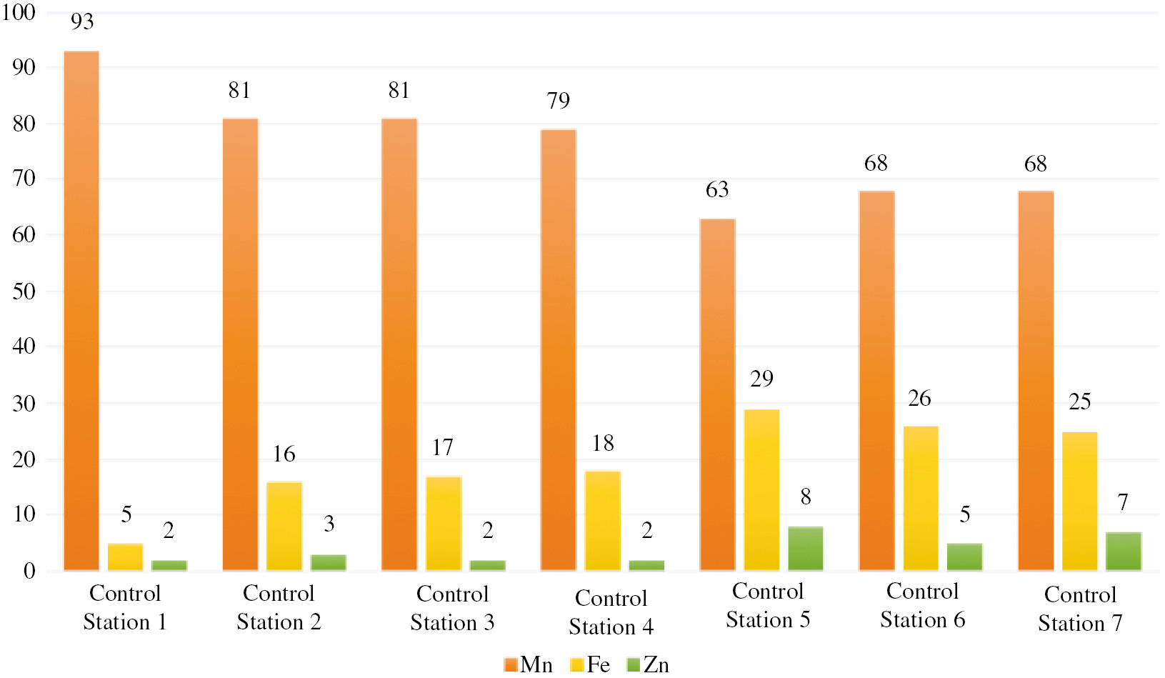
Priority of heavy metals in terms of their contribution to the water contamination index.
The previously reported approaches [6] have been used to estimate the mass fractions of the released contaminants. The release fraction of the ith contaminant in the jth river section between control stations can be determined using the following equation:
For each ith contaminant, the mass of released compound is determined by mass and flow rate according to the equation:
where vj is the incoming water volume in the jth river section per unit time, m3/s; Cij is the concentration of the ith contaminant in the jth river section.
Our estimate of the release of heavy metals in various segments of the Setun river has shown that the majority of manganese compounds enters the river in the territory of the Moscow region, between control stations 1 and 2 (Fig. 2).
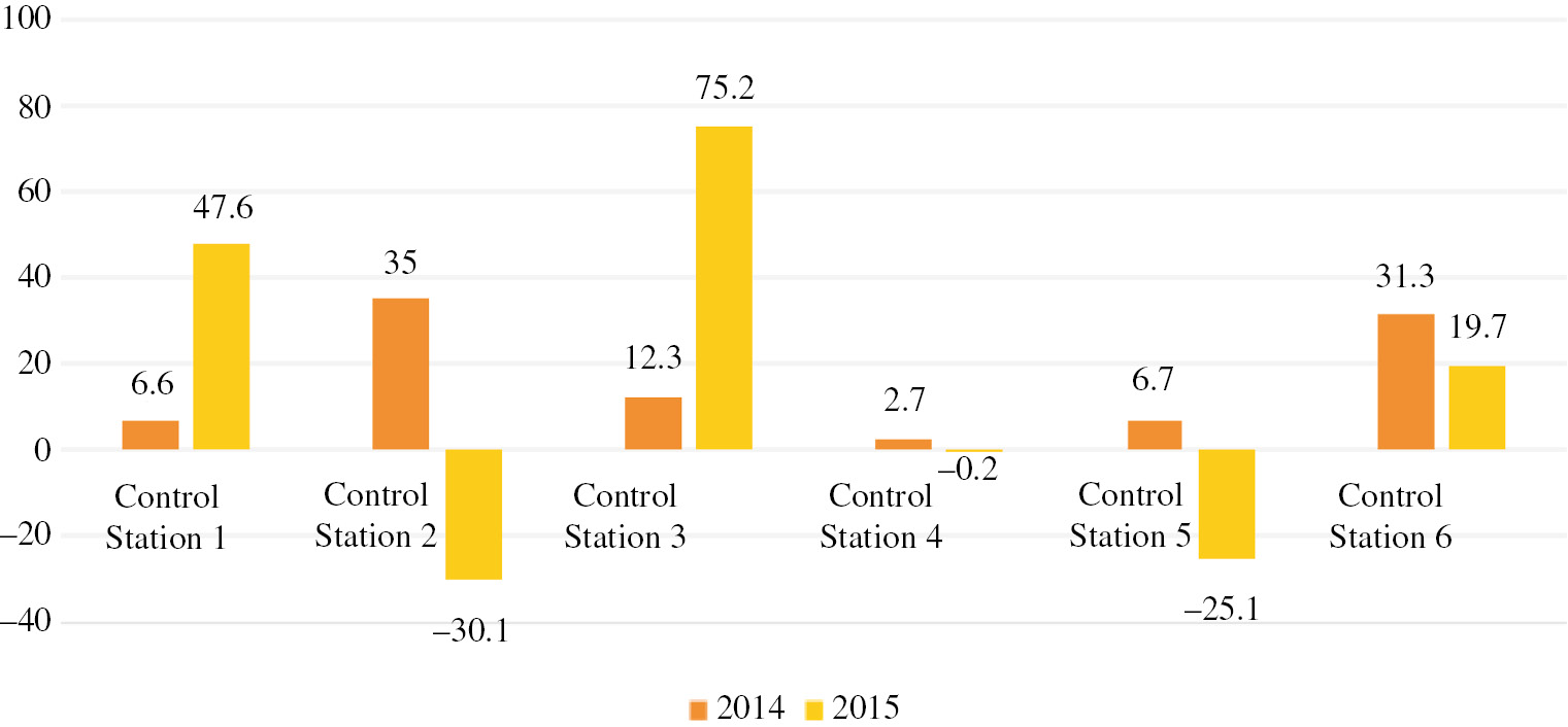
Mass fraction of manganese compounds released in various river parts.
The data obtained for the most hazardous contaminants and their points of entry along the river facilitate the selection of priority environmental solutions for decreasing the impact of heavy metals on the water object studied [7].
The analysis of the heavy metals concentrations in snow
Pollution of the environment with anthropogenic solid airborne particles is a global problem and study of solid airborne particles is of great importance for the problems of environment [8]. Snow is an ideal form of atmospheric precipitation for estimating the level of short-term seasonal emissions of various elements to the environment [9]. Studies were conducted in the Setun River Valley natural reserve. Samples were collected at all depths of the snow cover during its maximum accumulation.
Molten snow was filtered to separate the solid and liquid phases, which were analyzed separately. The results of the study were obtained by mass spectrometry with inductively coupled plasma (ICP-MS). Analysis of snow samples was performed on an XII-ICP-MS Thermo Scientific quadrupole mass spectrometer in the analytical laboratory of Institute of Geology of Ore Deposits, Petrography, Mineralogy and Geochemistry at the Russian Academy of Sciences. The results of the element analysis of solid phase of snow are given in Tables 3 and 4.
Rare earth element concentrations in snow.
| ppb | La | Ce | Pr | Nd | Sm | Eu | Gd | Tb | Dy | Ho | Er | Tm | Yb | Lu | La | La/Yb | Eu/Sm |
|---|---|---|---|---|---|---|---|---|---|---|---|---|---|---|---|---|---|
| 1 | 49.346 | 102.595 | 12.459 | 47.805 | 8.909 | 2.213 | 8.668 | 1.858 | 6.485 | 1.256 | 3.526 | 0.472 | 3.027 | 0.444 | 249.063 | 16.302 | 0.248 |
| 2 | 36.19 | 74.329 | 8.799 | 33.621 | 6.018 | 1.348 | 5.832 | 0.793 | 4.398 | 0.853 | 2.465 | 0.333 | 2.14 | 0.314 | 177.433 | 16.911 | 0.224 |
| 3 | 54.793 | 107.836 | 13.981 | 54.699 | 10.251 | 2.274 | 9.914 | 1.4 | 7.811 | 1.549 | 4.38 | 0.596 | 3.905 | 0.579 | 273.968 | 14.031 | 0.222 |
| 4 | 45.815 | 98.275 | 12.078 | 47.324 | 8.689 | 2.057 | 8.398 | 1.144 | 6.558 | 1.294 | 3.756 | 0.508 | 3.29 | 0.479 | 239.665 | 13.926 | 0.237 |
| 5 | 7.601 | 4.786 | 0.649 | 2.418 | 0.39 | 0.112 | 0.34 | 0.043 | 0.194 | 0.037 | 0.097 | 0.011 | 0.078 | 0.013 | 16.769 | 97.449 | 0.287 |
| 6 | 17.317 | 36.006 | 4.355 | 16.957 | 3.134 | 0.688 | 2.989 | 0.693 | 2.319 | 0.456 | 1.305 | 0.176 | 1.203 | 0.171 | 87.769 | 14.395 | 0.220 |
| 7 | 16.201 | 33.575 | 4.019 | 15.5 | 2.831 | 0.658 | 2.763 | 0.4 | 2.085 | 0.412 | 1.563 | 0.152 | 1.032 | 0.149 | 81.340 | 15.699 | 0.232 |
Metal concentrations in snow.
| ppb | V | Cr | Mn | Fe | Co | Ni | Cu | Zn | Sr | Mo | Cd | W | Tl | Pb |
|---|---|---|---|---|---|---|---|---|---|---|---|---|---|---|
| 1 | 307.41 | 172.57 | 1579.83 | 55024.91 | 51.19 | 446.69 | 296.74 | 1679.65 | 2125.50 | 12.66 | 2.42 | 129.09 | 1.92 | 69.27 |
| 2 | 159.03 | 94.91 | 693.53 | 24129.47 | 27.24 | 136.39 | 220.71 | 1079.84 | 1206.43 | 13.09 | 2.85 | 148.96 | 3.17 | 84.15 |
| 3 | 206.54 | 108.30 | 1120.19 | 43848.19 | 35.66 | 225.48 | 323.44 | 1146.05 | 1019.88 | 28.30 | 10.35 | 172.28 | 2.29 | 92.58 |
| 4 | 220.44 | 105.13 | 1041.58 | 40616.84 | 36.73 | 124.81 | 303.82 | 1006.96 | 1665.39 | 19.21 | 1.39 | 197.20 | 2.72 | 59.52 |
| 5 | 63.10 | 10.74 | 130.40 | 1450.35 | 3.23 | 109.48 | 38.15 | 351.67 | 88.84 | 1.73 | 1.07 | 4.10 | 0.17 | 10.96 |
| 6 | 96.46 | 45.33 | 67.34 | 10737.84 | 11.40 | 111.35 | 122.01 | 452.60 | 704.37 | 6.02 | 1.12 | 39.14 | 1.52 | 30.12 |
| 7 | 127.19 | 64.32 | 24.78 | 13655.00 | 13.96 | 103.10 | 496.13 | 637.81 | 338.04 | 7.37 | 0.96 | 43.48 | 1.42 | 34.10 |
The data obtained allow us to draw some conclusions about the content of the various elements and the nature of the distribution of rare earth elements (REE) in the snow samples studied. The total REE concentration (∑REE) varies from 0,017 to 0,249 ppm and decreases from southwest to northeast. The graphs of chondrite normalized REE concentrations showed negative REE distribution with La/Yb from 14 to 17 and Eu/Sm from 0.22 to 0.25 (Table 3, Fig. 3). Sample 5 is an exception; it has a minimum ∑REE (0.017 ppm) and an extremely high La/Yb=97 (Table 3, Fig. 3).
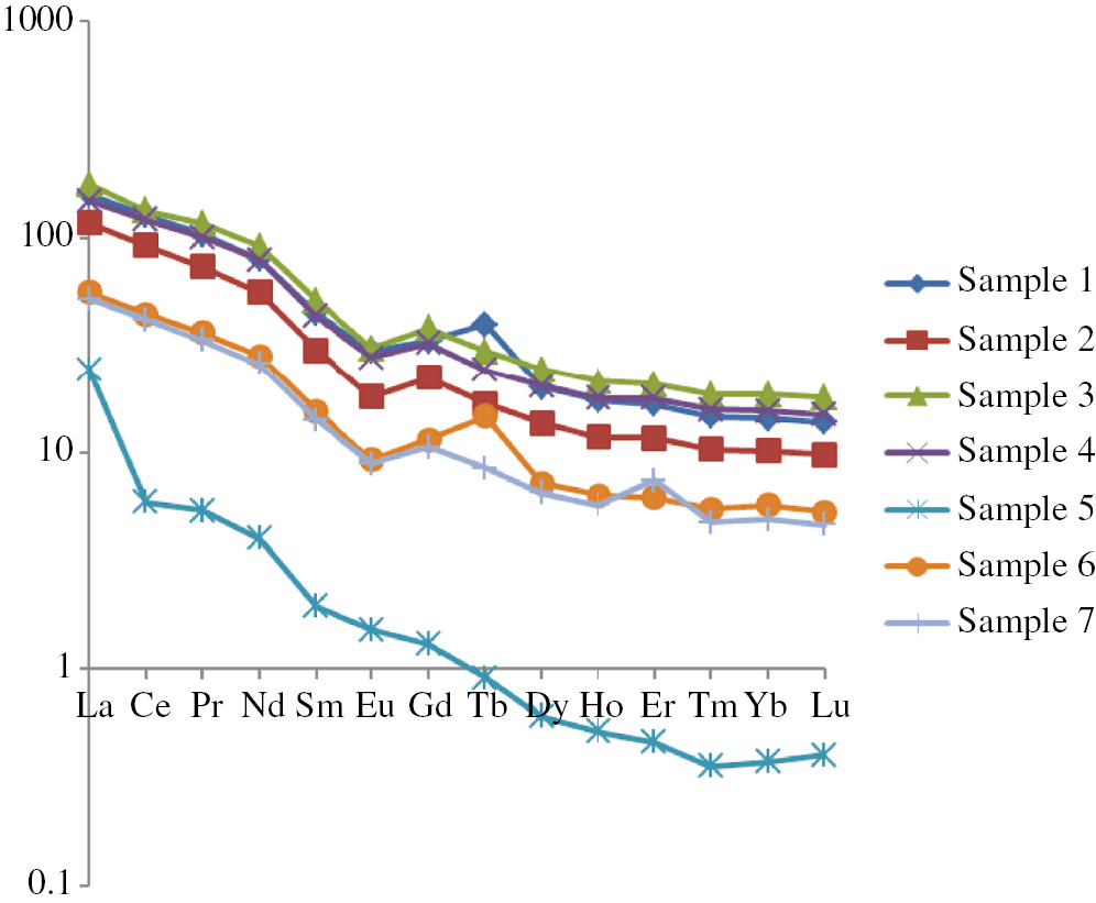
The graphs of chondrite normalized REE concentrations.
This analysis reveals a similar northeast directed downward trend in the content of heavy metals and some other toxic elements. The highest concentrations from 1.4 to 55.0 ppm are characteristic for Fe. It is also correlated with concentration of REE, Mn, Cr, Ni, Co, Pb and other elements (Table 4). Thus, a precise analysis of REE, heavy metals and other toxic elements concentrations and distribution in snow samples by ICP-MS provided an opportunity to assess the level of short-term seasonal eolian contamination in the Setun River Valley natural reserve. The data obtained are part of the ecological monitoring of this specially protected area. The results of the study may be applied to estimate the risks related to the contamination of the environment with heavy metals and other toxic elements.
The estimation of the environmental impact of heavy metals on the global and regional scales
The examples presented above are very illustrative. Rockström et al. [10], who introduced the concept of “planetary boundaries” that set a “safe functional space for the humankind” did not define a quantitative indicator for the “chemical pollution” planetary boundary. Instead, scientists consider several possible parameters that may determine these boundaries [11]. It is assumed that “chemical contamination” is not a unique and independent planetary boundary, but rather that there are a number of processes constituting a significant hazard on a planetary scale because of the chemicals in use. To avoid planetary problems related to the effects of chemical factors, it is necessary to develop a new global and proactive approach to identifying and managing the chemicals that could pose a threat to the entire planet. One of possible options for implementing such an approach is based on estimating the chemical footprint [12], which is most often defined as a quantitative measure describing the ecological space required to dilute the chemical contamination caused by human activity to a level below a defined threshold [13, 14]. This methodology is commonly used in Europe to estimate the impact of the production and use of chemicals [15], the chemical pollution in countries [12, 16], etc.
The evaluation of the adverse effects on the environment and human health caused by mercury mobilization
We applied a chemical footprint estimation methodology to determine the adverse effects on the environment and human health caused by mercury mobilization in the course of anthropogenic activity. Mercury, one of the most dangerous heavy metals, is a well-known hazardous contaminant [17]. Emissions and the discharge of mercury and its compounds create considerable risks both for the environment and for human health. The extent of the problems caused by mercury usage has been investigated, discussed, and received worldwide recognition at the Governing Council of the United Nations Environmental Programme (UNEP), culminating in the Minamata Convention on Mercury [18].
Contamination of mercury and its compounds is a consequence of human industrial activities [19]. According to estimates, about 2/3 of all the mercury circulating in the environment is of anthropogenic origin. Specialists’ estimates show that about 700 000 tons of mercury is human-made. A considerable fraction of this amount is found on the Earth’s surface.
There are four sources of mercury release/mobilization [17, 19]:
primary natural sources (volcanic activity, geothermal activity, the erosion of rocks containing mercury);
primary anthropogenic sources (ore mining and processing, waste incineration plants, cement kilns, large facilities for mining and producing non-ferrous metals (Cu, Zn, Pb, Al, Au, Ag), as well as the use of fossil fuels: coal, oil, etc.);
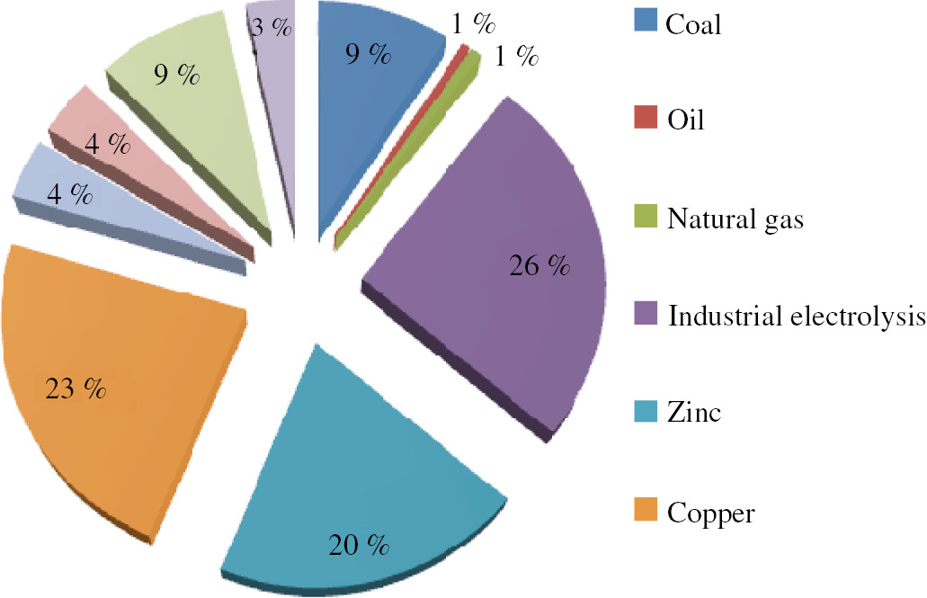
secondary anthropogenic sources (the use of power cells, paints, mercury thermometers, mercury light sources, and mercury as a cathode in electrolytic baths). Mercury is used as a catalyst or raw material in chemical and other industries, mercury and its compounds are present in various industrial and consumable products. Figure 4 depicts the approximate distribution of mercury usage among key industries around the world (data as of 2005) in metric tons;
re-mobilization (transfer of accumulated mercury from one domain to another, e.g. burning-out of forests or flooding of territories, since the biomass of forests and organic compounds of the surface layer of soil often contain mercury).
Distribution of mercury mobilization to the atmosphere in Russian Federation.
The Russian Federation considers the Minamata Convention on Mercury to be one of the key global environmental protection treaties developed under the auspices of UNEP in the past decade [15]. The interest of Russian Federation in this Convention is based on the fact that mercury contamination can have dangerous ecological consequences not only on local but also on regional scale [15]. Implementing the Minamata Convention on Mercury Provisions in the Russian Federation would minimize the risks of contamination with mercury and mercury compounds, provide for the recovery of polluted territories, and decrease mercury emissions in the atmosphere over the territory of the Russian Federation [15].
Figure 5 shows the locations of enterprises in the Russian Federation whose activity may result in potentially significant levels of mercury mobilization to the environment.
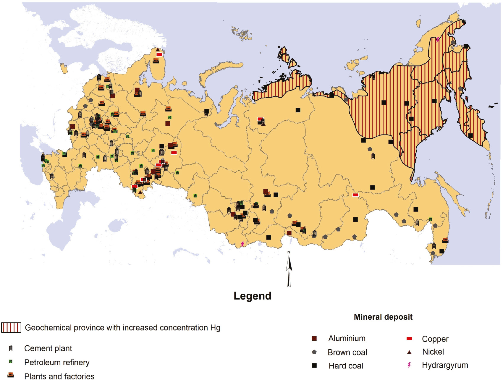
Main sources of mercury release into the environment.
The USEtox model developed by UNEP [20] is aimed to estimate the chemical pollution and chemical footprint. In order to estimate the significance of the impact of mercury and its compounds on the environment and health of the population in the Russian Federation, we have applied the USEtox model on the regional scale, e.g. the scale of federal districts of the Russian Federation. Calculations were carried out assuming that regional systems contain three components: atmospheric air, natural soils, and fresh waters (urban territories and sea waters were not taken into account).
Mean annual temperature, precipitation, river runoff, land area values have been provided by the Ministry of Natural Resources and Ecology of the Russian Federation [21, 22]. Mercury emission values, taken for the calculations, have been collected for the PCA/2013/030 GLF-2310-2760-4C83 grant “Pilot Project on the Development of Mercury Inventory in The Russian Federation”. Wind data have been provided by the European Centre for Medium-Range Weather Forecasts.
The mercury concentration values calculated for the components of the environment are presented in Table 5. The following officially established hygienic regulations for mercury and its compounds were used in the calculations: MAC in atmospheric air, daily average=0.0003 mg/m3 (with respect to mercury) [23]; MAC in fisheries=0.00001 mg/L [5]; MACsoil=2.1 mg/kg [24]. MAC for soil was recalculated with provided that the soil density was 2166.3 kg/m3 [25].
Mercury concentration values calculated for the components of the environment.
| Federal district | Mercury concentration (kg/m3) calculation results based on USEtox model |
||
|---|---|---|---|
| In air | In water | In soil | |
| North Caucasian | 2.35 · 10−14 | 4.64 · 10−8 | 7.10 · 10−3 |
| Central | 1.32 · 10−14 | 3.36 · 10−8 | 2.21 · 10−3 |
| Far Eastern | 5.76 · 10−15 | 1.13 · 10−8 | 2.95 · 10−4 |
| Siberian | 1.12 · 10−14 | 2.89 · 10−8 | 8.72 · 10−4 |
| Urals | 1.45 · 10−14 | 2.67 · 10−8 | 1.04 · 10−3 |
| Northwestern | 2.18 · 10−15 | 3.04 · 10−9 | 8.33 · 10−5 |
| Volga (Privolzhsky) | 2.48 · 10−14 | 5.14 · 10−8 | 4.56 · 10−3 |
| Southern | 6.03 · 10−15 | 8.57 · 10−9 | 1.85 · 10−3 |
| MACs | 3.00 · 10−10 | 1.00 · 10−8 | 4.55 · 10−3 |
The calculated concentrations of mercury for soil exceed MAC in Volga and North Caucasian federal districts. The calculated concentrations of mercury for fishery water bodies exceed MAC in all federal districts.
The assessment of the impact of climate change and national regulation on the mercury concentration in the components of the environment
We have also calculated concentrations of mercury for the year 2045 assuming representative concentration pathways RCP4.5 (the scenario adopted by the Intergovernmental Panel on Climate Change (IPCC) [26]) and corresponding predictions for temperature, wind and precipitation produced by the Institute of Numerical Mathematics (INM RAS) CM4 model [27] for the Coupled Model Intercomparison Project (CMIP5). The RCP 4.5 is a stabilization scenario where total radiative forcing is stabilized before 2100 by employment of a range of technologies and strategies for reducing greenhouse gas emissions [28].
We have concluded that due to significant increase of precipitation in the federal districts of the Russian Federation mercury concentration would decrease in epy atmospheric air (by 22%), in small water bodies (by 12%), and in soil (by 12%), but would respectively increase in seas and oceans [29]. Despite of the above-mentioned decrease, the average mercury concentration in the federal districts would still exceed the established MACs, so additional regulative steps should be taken by the government.
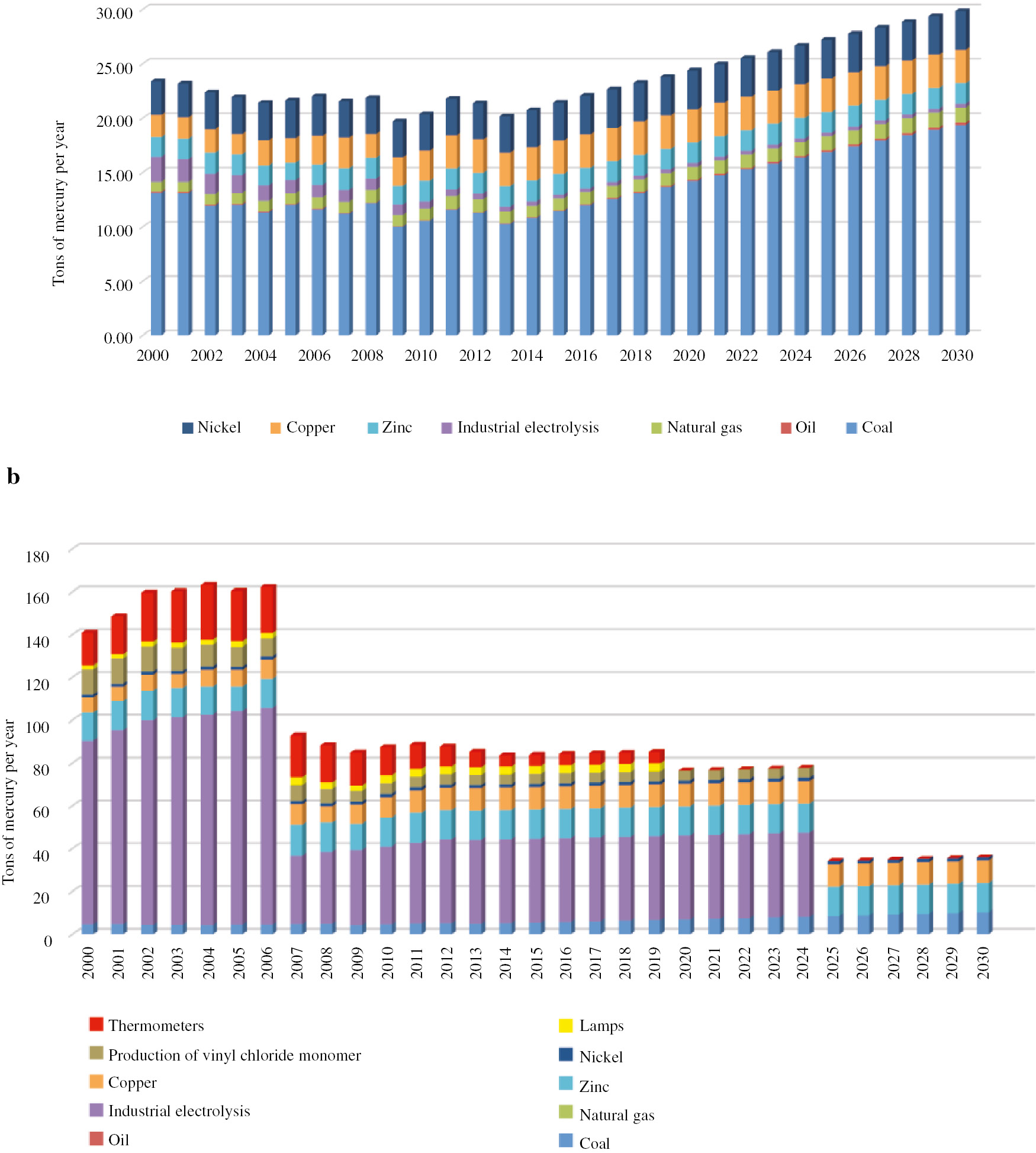
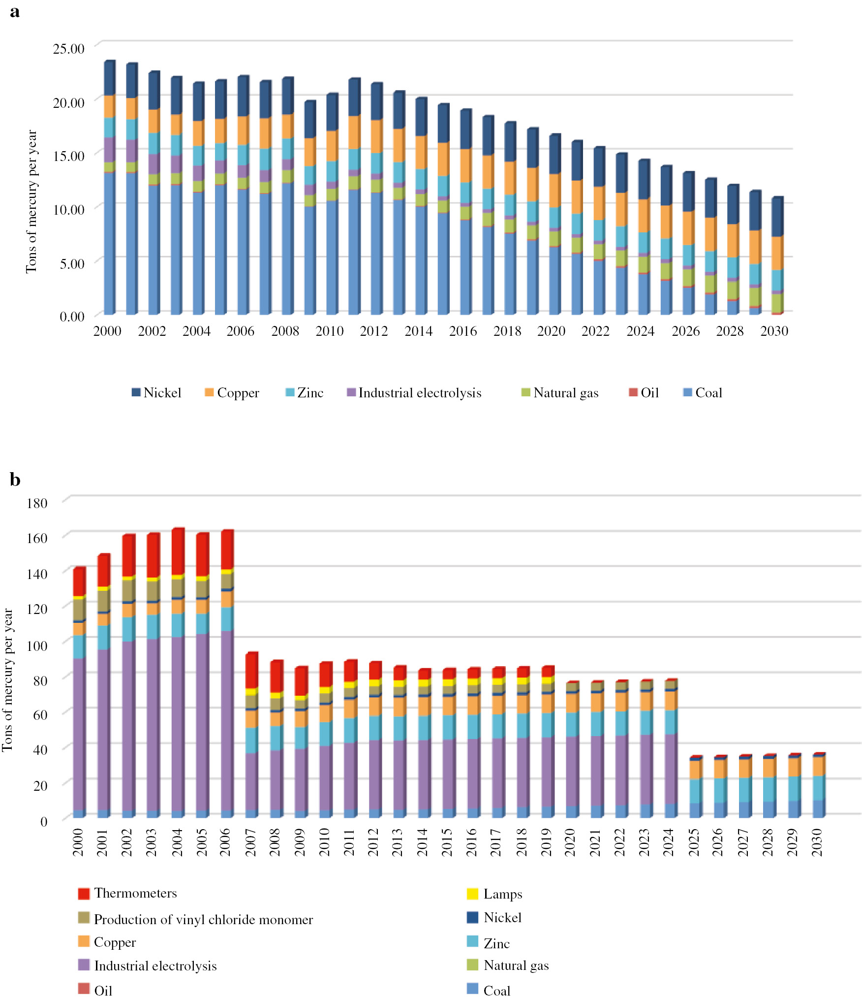
Several scenarios have been considered for the proposals of a national action plan to minimize mercury exposure. The effects of government regulatory systems on minimizing exposure to mercury and its compounds can be seen in Figs. 6–8. In order to perform such an assessment, sources of potential mercury mobilization in the Russian Federation have been identified, and a model has been constructed which predicts the levels of emissions and discharges of mercury depending on decisions made at the national level.
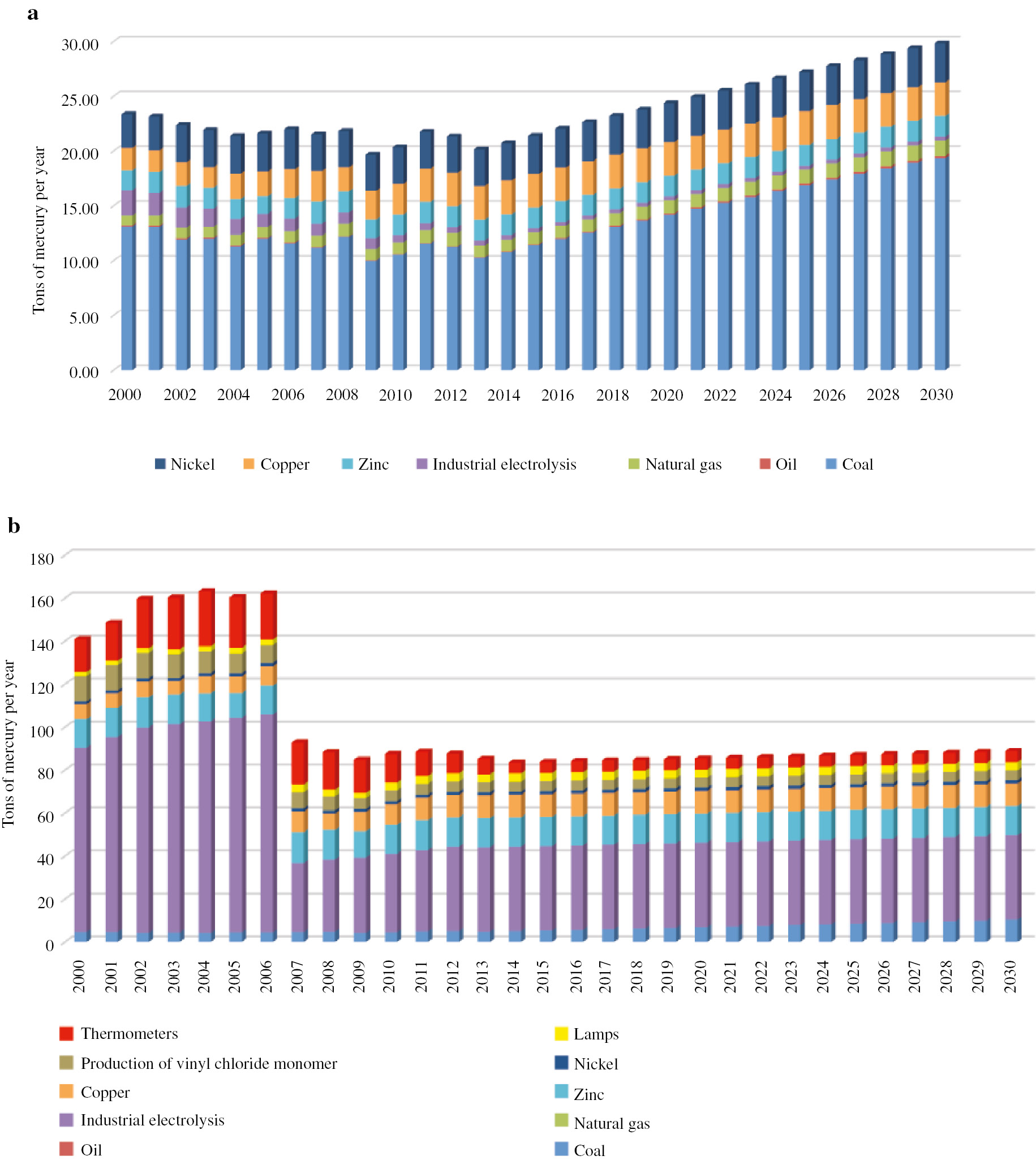
(a) Mercury emission and (b) mercury in waste (scenario 1).
(a) Mercury emission and (b) mercury in waste (scenario 2).
(a) Mercury emission and (b) mercury in waste (scenario 3).
The first scenario corresponds to the situation when the government does not interfere in the regulation of mercury circulation, but still runs industry and energy development programs launched in Russia. The graphs presented in Fig. 6 show a noticeable increase in mercury emissions to the atmosphere and mercury waste generation.
In the second scenario, the government follows the regulatory activities laid out by the Minamata Convention on Mercury. The graphs presented in Fig. 7 show that employing these activities will lead to a minimization of waste generation; this in turn, directly corresponds with one of the key principles of green chemistry.
In the third scenario, aside from compliance with Minamata objectives, the government will conserve resources in addition to increasing energy efficiency by replacing coal with more environmentally friendly natural gas, with the results being even more impressive in the long run (see graphs presented in Fig. 8). It will not only be possible to reduce levels of toxic waste, but also to obtain a reduction of mercury emissions into the environment.
The superposition of RCP 4.5 scenario and the scenario of Minamata convention governmental implementation (prohibition to release to the environment mercury utilized as industrial catalysts, mercury from lamps and other appliances) predicts that the average mercury concentration in soil would be less than the established MAC for mercury concentration by 2045. The average mercury concentration in atmosphere reduces by 33% with the maximal reduction in the South and the North-western federal districts (by 57%) and minimal reduction in the Urals and the North Caucasian federal districts (by 17–18%). The average concentration of mercury in water bodies also reduces by 21% with the maximal reduction in the South federal district (by 93%) and the minimal reduction in the Urals federal district (by 7%) though still exceeding maximal allowable concentrations in all districts except the South and the North-Western districts.
In conclusion, it is necessary to mention that scientific and technological community is one of nine sectors of society (“Major Groups”) formalized as the main channels through which broad participation would be facilitated in the UN activities related to sustainable development. Among the approaches in the field of SD, developed by the community recently, the concept of planetary boundaries might be mentioned as a powerful tool to facilitate analysis of the consequences of the anthropogenic impact on the environment. “Chemical pollution” is one of two planetary boundaries that has not been quantified (because of its’ complexity). The fate of heavy metals (including the rare earth metals) in the environment might serve as an example of this complexity. Never-the-less, the monitoring data allow to rank the levels of pollution with different heavy metals and to identify their sources, as well as to analyse different scenario of the industrial policy.
Article note
A collection of invited papers based on presentations at the 6th international IUPAC Conference on Green Chemistry (ICGC-6), Venice (Italy), 4–8 September 2016.
Acknowledgments
This research was partially supported by the Russian Science Foundation, grant 15-17-30016.
References
[1] United Nations A/RES/70/1. Transforming our world: the 2030 Agenda for Sustainable Development. Resolution adopted by the General Assembly on 25 September 2015. United Nations Sustainable Development Knowledge Platform (2015). URL: sustainabledevelopment.un.org/index.php?menu=2361. Accessed 12 March 2016.Search in Google Scholar
[2] W. Steffen, K. Richardson, J. Rockström, S. E. Cornell, I. Fetzer, E. M. Bennett, R. Biggs, S. R. Carpenter, W. de Vries, C. A. de Wit, C. Folke, D. Gerten, J. Heinke, G. M. Mace, L. M. Persson, V. Ramanathan, B. Reyers, S. Sörlin. Science347, 1259855 (2015).10.1126/science.1259855Search in Google Scholar
[3] P. Gupta, A. Mahajan. RSC Adv.5, 26686 (2015).10.1039/C5RA00358JSearch in Google Scholar
[4] P. Gupta, S. Paul. Catal. Today236, 153 (2014).10.1016/j.cattod.2014.04.010Search in Google Scholar
[5] Federal Fisheries Agency. Order of the Federal Fisheries Agency no. 20 as of January 18, 2010 on the approval of the standards of water quality in water bodies of commercial fishing importance, including the standards of maximum allowable concentrations of hazardous compounds in the waters of the water bodies of commercial fishing importance. Moscow (2010).Search in Google Scholar
[6] B. A. Kuznetsov, N. P. Tarasova, A. E. Biryukov. Ecology of the Urbanlzed Territories2, 100 (2008).Search in Google Scholar
[7] A. V. Dubinin. Rare Earth Elements in the Ocean, I. I. Volkov (Ed.), Nauka Press, Moscow (2006).Search in Google Scholar
[8] A. V. Talovskaya, E. G. Yazikov, E. A. Filimonenko, N. P. Samokhina, T. S. Shakhova, I. A. Parygina. Atmos. Ocean Opt. Atmos. Phys.10035, 100354F (2016). URL: earchive.tpu.ru/handle/11683/38247 (accessed 22 August 2017).Search in Google Scholar
[9] S. F. Vinokurov, D. B. Petrenko, V. A. Sychkova, N. P. Tarasova. Doklady RAS Earth Sci.456, 602 (2014).10.1134/S1028334X14050389Search in Google Scholar
[10] J. Rockström, W. Steffen, K. Noone, A. Persson, F. S. Chapin, E. F. Lambin, T. M. Lenton, M. Scheffer, C. Folke, H. J. Schellnhuber, B. Nykvist, C. A. de Wit, T. Hughes, S. van der Leeuw, H. Rodhe, S. Sorlin, P. K. Snyder, R. Costanza, U. Svedin, M. Falkenmark, L. Karlberg, R. W. Corell, V. J. Fabry, J. Hansen, B. Walker, D. Liverman, K. Richardson, P. Crutzen, J. A. Foley. Ecol. Soc.14, 32 (2009).10.5751/ES-03180-140232Search in Google Scholar
[11] L. M. Persson, M. Breitholtz, I. T. Cousins, C. A. de Wit, M. MacLeod, M. S. McLachlan. Sci. Technol.47, 12619 (2013).10.1021/es402501cSearch in Google Scholar
[12] A. Bjørn, M. Diamond, B. Birkved, M. Z. Hauschild. Environ. Sci. Technol.48, 13253 (2014).10.1021/es503797dSearch in Google Scholar
[13] A. Adriaanse. Environmental Policy Performance Indicators, S.D.U., Hague (1993).Search in Google Scholar
[14] M. C. Zijp, L. Posthuma, D. van de Meent. Environ. Sci. Technol.48, 10588 (2014).10.1021/es500629fSearch in Google Scholar
[15] United Nations. 69th session of the General Assembly. Speech by deputy of Natural Resources and Ecology of the Russian Federation RR Gizatulina at the signing ceremony the Minamata Convention on Mercury. October 25, 2014 UN Headquarters, New York City. URL: russiaun.ru/ru/news/cnv_gza (accessed 12 March 2017).Search in Google Scholar
[16] N. P. Tarasova, A. S. Makarova. Russ. Chem. Bull. Int. Ed.65, 1 (2016)10.1007/s11172-016-1467-zSearch in Google Scholar
[17] J. Weinberg. NGO Introduction to Mercury Pollution. IPEN URL: www.ipen.org/documents/ngo-introduction-mercury-pollution (accessed 12 March 2017).Search in Google Scholar
[18] J. Roberts. Minamata Convention enters force in August. Chemical Watch, Global Business Briefing – July/August 2017. URL: chemicalwatch.com/57847/ (accessed 22 August 2017).Search in Google Scholar
[19] UNEP. Toolkit for Identification and Quantification of Mercury Releases. UNEP URL: www.unep.org/chemicalsandwaste/Mercury/ReportsandPublications/MercuryToolkit (accessed 12 March 2017).Search in Google Scholar
[20] T. B. Westh, M. Z. Hauschild, M. Birkved, M. S. Jørgensen, R. K. Rosenbaum, P. Fantke. Int. J. Life Cycle Assess.20, 299 (2015).10.1007/s11367-014-0829-8Search in Google Scholar
[21] Ministry of Natural Resources and Ecology of the Russian Federation. Public report on the state and use of Russian Federation mineral resources in 2012. Moscow (2013).Search in Google Scholar
[22] Ministry of Natural Resources and Ecology of the Russian Federation. Public report on the state and use of Russian Federation water resources in 2014. Moscow (2015).Search in Google Scholar
[23] Rospotrebnadzor. Maximum allowable concentrations (MAC) of pollutants in the atmospheric air of populated areas: Health standards. Moscow. GN 2.1.6.1338-03 (2003).Search in Google Scholar
[24] Rospotrebnadzor. Maximum allowable concentrations (MAC) of chemical compounds in soil: Health standards. Moscow. GN 2.1.7.2041-06 (2006). ISBN 5-7508-0599-9.Search in Google Scholar
[25] UNEP/SETAC. USEtox® 2.0 Documentation (Version 1). ISBN: 978-87-998335-0-4, DOI: 10.11581/DTU:00000011. http://www.usetox.org/sites/default/files/assets/USEtox_Documentation.pdf Accessed 12 March 2017 (2017).10.11581/DTU:00000011Search in Google Scholar
[26] J. Weyant, C. Azar, M. Kainuma, J. Kejun, N. Nakicenovic, P.R. Shukla, E.La Rovere, G. Yohe. Report of 2.6 Versus 2.9 Watts/m2 RCPP Evaluation Panel. Geneva, Switzerland: IPCC Secretariat. web. http://www.ipcc.ch/meetings/session30/inf6.pdf (2009).Search in Google Scholar
[27] E. M. Volodin, N. A. Diansky, A. V. Gusev. Izvestiya Atmos. Ocean. Phys.46, 414 (2010).10.1134/S000143381004002XSearch in Google Scholar
[28] L. Clarke, J. Edmonds, H. Jacoby, H. Pitcher, J. Reilly, R. Richels. Scenarios of Greenhouse Gas Emissions and Atmospheric Concentrations. Sub-report 2.1A of Synthesis and Assessment Product 2.1 by the U.S. Climate Change Science Program and the Subcommittee on Global Change Research, pp. 154. Department of Energy, Office of Biological & Environmental Research, Washington, USA (2007).Search in Google Scholar
[29] S. Jonsson, A. Andersson, M. B. Nilsson, U. Skyllberg, E. Lundberg, J. K. Schaefer, S. Åkerblom, E. Björn. Sci. Adv.3, 1 (2017).10.1126/sciadv.1601239Search in Google Scholar
©2018 IUPAC & De Gruyter. This work is licensed under a Creative Commons Attribution-NonCommercial-NoDerivatives 4.0 International License. For more information, please visit: http://creativecommons.org/licenses/by-nc-nd/4.0/
Articles in the same Issue
- Frontmatter
- In this issue
- Conference papers
- Papers from the 6th International IUPAC Conference on Green Chemistry (ICGC-6)
- Microwave assisted synthesis of glycerol carbonate from glycerol and urea
- Silica gel mediated oxidative C–O coupling of β-dicarbonyl compounds with malonyl peroxides in solvent-free conditions
- Definition of green synthetic tools based on safer reaction media, heterogeneous catalysis, and flow technology
- Heavy metal removal from waste waters by phosphonate metal organic frameworks
- A clean and simple method for deprotection of phosphines from borane complexes
- Development and treatment procedure of arsenic-contaminated water using a new and green chitosan sorbent: kinetic, isotherm, thermodynamic and dynamic studies
- Bio-adsorbent derived from papaya peel waste and magnetic nanoparticles fabricated for lead determination
- 5-Membered cyclic ethers via phenonium ion mediated cyclization through carbonate chemistry
- Synergy in food, energy and advanced materials production from biomass
- Step economy strategy for the synthesis of amphoteric aminoaldehydes, key intermediates for reduced hydantoins
- Separation technology meets green chemistry: development of magnetically recoverable catalyst supports containing silica, ceria, and titania
- Green chemistry and sustainable development: approaches to chemical footprint analysis
- Greener solvents for solid-phase organic synthesis
- Photocatalytic hydrogenolysis of allylic alcohols for rapid access to platform chemicals and fine chemicals
- IUPAC Recommendations
- Definition of the mole (IUPAC Recommendation 2017)
- Terminology of separation methods (IUPAC Recommendations 2017)