Pottery from Motion – A Refined Approach to the Large-Scale Documentation of Pottery Using Structure from Motion

1 Introduction

In 2021, Göttlich et al. (2021) presented a new large-scale documentation method using the three dimensional (3D)-capture method structure from motion (sfm) to document pottery sherds. They argued that this documentation methodology is significantly faster than the traditional method of drawing while simultaneously being more affordable. However, the methodology was only tested in a minimal timeframe (a couple of days), while only one pottery group (Phoenician amphorae) was photographed and only partly processed.

With the 2021 article as a starting point, a follow-up study was conducted in 2022 and 2023 to see how well this method performs in a large-scale documentation context dedicated solely to the documentation of pottery as 3D models including more complex structures such as handles, tableware (pottery consisting of plates and bowls) as well as painted pottery (such as Greek imports). The results confirm that this methodology truly delivers a fast and precise documentation but the characterization of being “low-cost” has to be questioned. Additionally, it was possible to improve the overall workflow, reduce variability regarding results, and achieve reliable and high-quality 3D models in a short amount of time. However, it is best used for rather quantitative analysis methods and not for the sole documentation of all excavated pottery sherds as I will show throughout this article.

Next to testing this workflow and presenting our results, two additional objectives concerning sfm, which have been neglected so far, will be addressed here. The first objective is to present a detailed walkthrough of the methodology. 3D-related methods and photogrammetry are becoming more and more common in university teaching, but they are still insufficiently represented. At many universities, this methodology is connected mainly to designated fields of study such as cultural heritage or digital humanities and occurs relatively isolated in a student’s CV. In my experience, studies mostly rely on specialists while students have to be lucky to gather limited experience during relatively isolated courses or during excavation season. Specialists are more costly and can only manage a certain amount of work alone. Excavations are – in my opinion – hardly the time and space to explain aspects of photogrammetry in detail since time is heavily limited and respective situations have to be met with spontaneous problem-solving, which often requires a specific set of beforehand experiences. Consequently, this article is mainly addressed to new users in the field of photogrammetry who want to conduct this methodology^[1] presented by Göttlich et al. (2021) since the information they give is relatively scarce. Missing, for example, are detailed descriptions of technical aspects (e.g., the camera settings or camera set-up), and crucial steps regarding the workflow while processing the models are discussed fairly limited. This prevents reproducible results, hinders a deeper understanding of the individual steps of the workflow, and encourages people to rely entirely on the respective software algorithms without knowing what is happening. Consequently, the workflow of documenting pottery via sfm and processing them with the respective software will be presented in detail to give new users a manual (see Appendix).

The second objective of this article is to critically discuss the necessity of documenting hundreds or even thousands of seemingly similar pottery sherds as 3D models since data management rises significantly and equipment (on and off-site) is relatively expensive (see below), even though it is often considered to be “low-cost” (Göttlich et al., 2021, p. 257). Here, the key differences between the traditional method and digital methods, such as the “laser-aided profiler” (LAP) (Demján et al., 2022), as well as sfm, will be discussed, including its limitations and benefits. I will show that this methodology does not – at the current state – qualify for the singular documentation of all excavated pottery sherds from a respective site but as an additional methodology with a quantitative research approach in mind. Ultimately, I will argue that a constant comparison of traditional or digital drawing and 3D modeling methodologies is equally senseless since the produced outcome differs significantly from each other. Lastly, the statement regarding low cost has to be put in the respective research perspective while generally characterizing this methodology as low-cost is not correct.

The material of this study consists of Phoenician amphorae (now included with more complex surface structures such as handles and complete profiles), painted and unpainted tableware pottery, as well as Greek and Cypriote imports excavated in the settlement of Tell el-Burak at the Lebanese coast south of Beirut. The amphorae are currently being studied by Aaron Schmitt and his team (University of Heidelberg) (first results see Di Angelo et al., 2024; Schmitt et al., 2019). Greek imports are studied by Maximilian Rönnberg and Cypriote imports by Meryem Bueyuekyaka (Rönnberg et al., 2023). I am currently analyzing the tableware vessels within the scope of my ongoing PhD project.

2 sfm as a Documentation Method of Pottery

sfm can be defined as extracting information from two-dimensional ([2D] and overlapping) pictures to reconstruct a 3D structure. It is often characterized as “[…] the computer vision equivalent of a human’s ability to understand the 3D structure of a scene as they move through it” (Green et al., 2014, p. 173; Szeliski, 2022). 3D methods such as sfm, laser scanning, or structured light scanning are widely used for the documentation of entire excavation sites or even buildings (see, for example, Green et al., 2014; Jones & Church, 2020), smaller objects such as small finds (Breuer et al., 2020), and also pottery (Barreau et al., 2014; Göttlich et al., 2021; Karasik & Smilansky, 2008; Wilczek et al., 2018).

The method Göttlich et al. (2021) proposed contained the usage of a DSLR Camera paired with a so-called “pottery tree” and was specifically designated for the documentation of pottery. The pottery tree consists of a vertical rod with three horizontal rods carrying a clamp on each side. The idea is to photograph the entire structure as a singular 3D object while pottery sherds are attached to each clamp (Göttlich et al., 2021, Figure 7). Through this approach, several sherds (in this case eight) can be documented simultaneously, which was then compared to the documentation time needed for traditional drawings.

A similar approach was already proposed by Karasik and Smilansky (2008) but differed in the structure of the “pottery tree” (Karasik & Smilansky, 2008, Figure 2) as well as in the usage of a structured light scanner (Karasik & Smilansky, 2008, p. 1150). A later study by Wilczek et al. (2018) also used a structured light scanner. Wilczek et al. (2018) documented singular sherds, while Karasik and Smilansky (2008) documented more than one sherd simultaneously (6–7 sherds) on their version of the “pottery tree” (Karasik & Smilansky, 2008, Figure 2). The set-up proposed by Karasik and Smilansky (2008) seems rather spacious and together with the structured light scanner and – in this specific case – the constant need for electricity, this method hardly seems feasible if longer traveling and difficult surroundings are present. Newer models of structured light scanners also run with batteries and could equally be used, but remain rather expensive.^[2] Here, I assume that the structure of the pottery tree (as can be seen in Figure 1) needs to be altered to provide an efficient workflow to facilitate documentation. This, however, should be tested in a separate study as this one specifically focuses on the methodology presented by Göttlich et al. (2021). Every item Göttlich et al. (2021) use is easy to carry and travel with. Additionally, the workflow can be conducted in smaller spaces efficiently, while solely using electricity provided by rechargeable batteries.

Figure 1

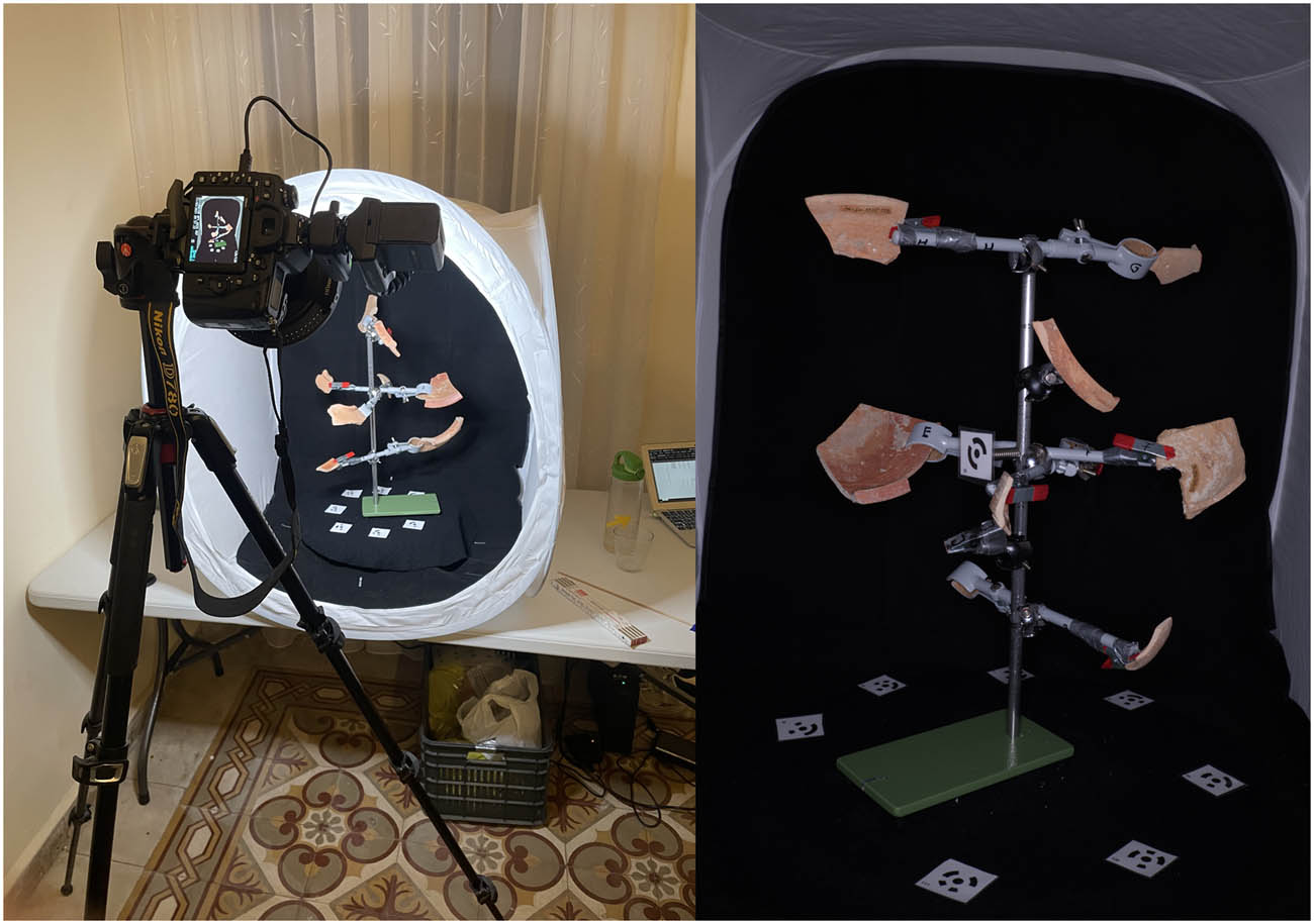
Depiction of a set-up including a close-up photograph of a pottery carrying eight clamps.

Göttlich et al. (2021), Karasik and Smilansky (2008), and Wilczek et al. (2018) share the intended result. The first two studies aimed to use 3D models to produce a profile drawing, similar to traditional drawing or the LAP, and to orientate the sherd automatically. Consequently, the result would be identical to (traditional or digital) drawing. Göttlich et al. (2021) intended to use the entire (orientated) 3D model as a result for publication but also proposed the creation of a digital 2D drawing that derives from the 3D model using the software “TroveSketch” and “Vessel Reconstructor” (Göttlich et al., 2021, p. 266). Additionally, they compared the needed documentation time with the traditional method.

As mentioned before, our study focused on the reproducibility of the method presented by Göttlich et al. (2021), with the difference that there are – for now – no intentions of producing computer-assisted drawings.^[3] In our case, the 3D models are used to obtain measurements, regarding their respective morphometric vessel features such as diameter, preservation, thickness (rim and wall), inclination (rim, wall, shoulder), and so on. Those measurements can be used to analyze certain parameters of production such as standardization to postulate assumptions about – for example – specialization (Blackman et al., 1993; Gandon et al., 2018; Gandon et al., 2020; Harush et al., 2020; Roux, 2003). To do this, statistical calculations such as the coefficient of variation (based on the variation of parameters) or statistical tests^[4] deriving from the field of statistical inference are needed. These tests, however, need specific requirements and – mostly large – neutral, precise, and accurately documented data. For example – in the case of my PhD thesis – the 3D models are used to obtain measurements from them – regarding their respective morphometric vessel features (diameter, preservation, thickness, inclination, etc.). The results are used to conduct the above-mentioned analysis (e.g., multivariate analysis of variance [MANOVA]) to compare morphometric parameters between different assemblages and types excavated at different Phoenician sites to postulate assumptions about the organization of production throughout the late Iron Age. To obtain these fine measurements in the most neutral, accurate, and precise manner, the 3D models are measured automatically. This is done via software provided by Prof. Luca Di Angelo and Prof. Paolo Di Stefano from the University of L’Aquila, Italy (Di Angelo et al., 2018, 2020, 2024). In this example textures of 3D models are not used or processed, meaning only a specific aspect of this documentation is utilized in our case. However, processing models with texture or without holes still remain possible as all needed information is documented through the described workflow and respective raw material (see below).

3 Göttlich et al. (2021) and Case Studies of 2022 and 2023

The following text only focuses on the “3D models” aspect of the paper by Göttlich et al. (2021, pp. 263–271) to present significant changes and additional detail on how to conduct this methodology. As mentioned above, the focus here lies on how to do this in greater detail, as well as to present the changes that were implemented in the method. I will first give an overview of the “on-site” documentation method presented by Göttlich et al (2021), followed by our case study as well as the changes we conducted. Following this, I will again present the “off-site” (processing) documentation given by Göttlich et al. (2021), which is again followed by our workflow and the respective changes. The last aspect of this article will be a brief discussion of the method in comparison to manual and digital drawing.

Göttlich et al. refer to the 3D documentation and mention the needed equipment, which consists of a DSLR-Camera^[5] (Canon EOS 70D), fixed focal length of 35 mm, a tripod, a light tent, a turntable, the “pottery tree,” as well as the general set-up of all mentioned equipment (2021, pp. 264–265). Only a very fragmentary description of the set-up is given, and no technical information such as aperture, shutter speed, sensor size, or white-balancing is presented. Photographs were taken in landscape mode which is not mentioned but visible through pictures provided by the authors (Göttlich et al., 2021, Figures 8 and 10). Photographs of the sherds were conducted in bright shade, avoiding direct sunlight, using a light tent with a black background. The so-called markers are placed on the turntable from which the distance is taken to reference the 3D models. Camera calibration (to counter several distortion parameters such as lens distortion) was done once a day using the checkerboard calibration provided by the software. Camera placement is only referred to as a range between 50 and 100 cm, depending on the lens. The text does not mention any reason for this beyond the information that this distance differs in relation to different lenses (Göttlich et al., 2021, p. 264).

Every tree was photographed twice to document the area of the sherds, which was covered by the clamp. Each pass contains roughly 90–100 shots in total. A total of 23–25 shots are conducted per revolution of the turntable. This is repeated in four different angles of height (Göttlich et al., 2021, 265, Figure 9). In both directions – horizontally and vertically – an overlap of 80% has to be ensured for a complete calculation of the object surface (Göttlich et al., 2021, p. 265).

In March 2022, a 4-week follow-up study was conducted in Beirut to document a large number of undocumented amphorae and tableware from the excavation site of Tell el-Burak, solely with the use of sfm. A second shorter campaign was conducted in November 2022 (8 full workdays) and another 4-week campaign in March 2023. In March 2022, two pottery trees with eight clamps each were used. In November 2022, tests were conducted with 10 and 12 clamps, which drastically maximized the number of documented sherds. This test was limited to smaller sherds, but documenting larger pottery fragments is technically possible. In March 2023, several combinations of eight and ten clamps were used.^[6]

Every tree was assigned an individual ID, and all clamps were assigned letters from A to H to identify the respective sherds based on their positioning. During the photo sessions, the following information was recorded in the “tree list”: tree ID, clamp ID, sherd ID, target ID, and the measured distances between the targets.

Two of the set-ups (Figure 1) were used during our study, allowing us to document a minimum of eight sherds per tree simultaneously. Two people worked at every station. One person photographed while the other prepared the next tree and repacked the documented sherds. Positioning one person per station is possible, but this negatively affects efficiency because no photography takes place while a new tree is being prepared. Additionally, a second person at every station can check every step while being cross-checked by their partner. This lowers the risk of mistakes. Another possibility would be to use three people, namely two photographers and one assistant, servicing both stations. However, the most efficient way proved to be two persons per station.

3.1 Set-up and Settings

Concerning the equipment used for photography, we followed the recommendations given by Göttlich et al. (2021, p. 264) with small but significant changes. The first change was to use a full-frame camera (Nikon D780) with 24.3 MP instead of a camera with an APS-C or crop sensor (such as the camera used by Göttlich et al. (2021), which only has 20.3 MP). A full-frame sensor enhances quality since the individual pixels on the sensor are larger. Larger pixels catch more light and consequently more detail which leads to better results (Newton, 2022). Additionally, a higher pixel number enhances the quality of pictures because of more pixels, catching more light and therefore more information. On the downside, more pixels (especially large ones) produce larger files. Additionally, full-frame cameras are generally more expensive than cameras with an APS-C or crop sensor.

The second change was to take shots in portrait rather than landscape mode. If the latter is used, much sensor space is wasted on the black background on the right and left of the pottery tree, due to its elongated vertical structure. Photographing in portrait mode enables us to use the sensor space (and the respective pixels) more efficiently, which strengthens the model structure and enables us to always photograph all attached sherds on the tree.

The third change was to slightly elevate the pottery tree inside the tent (roughly 10 cm) to provide more exposure to the camera at steep angles from below. Referencing is done via the so-called markers which were glued on the outer rim at ca. 10–15 cm intervals. Distance between the markers was measured with a ruler and recorded in 1 mm steps. Accepted deviations of manual measuring distance are consequently ±0.5 mm (Taylor, 1982, pp. 8–9).

As mentioned above, camera settings are not mentioned at all by Göttlich et al. (2021). This is problematic and hinders reproducibility because the settings have a critical impact on the results. In our case, the camera was set to manual (M) to control the settings fully.^[7] The auto-focus is set to a single focus point as well as the AF single-mode. Metering is set to single-spot measuring. ISO value was set to 100. The aperture was set to f/16^[8] to achieve a large depth of field, enabling us to have all the sherds of the “pottery tree” in focus. Due to the geometry of the pottery tree, it is hardly possible to have all sherds inside the depth of field at all times. This represents a significant structural problem, which will be explained below. The shutter speed should be increased to compensate for the small aperture. This, however, heavily depends on the lighting in the respective surroundings. If a ring light (diffuse lightning) is used, longer exposure times can be avoided, but a tripod and a remote switch are still necessary to prevent shaking the camera. The chosen shutter speed was between 1/1.6 and 1/4 s.

Another change was to photograph inside a darkened room. Photographing in bright shades, as proposed by Göttlich et al. (2021, p. 264), proved inefficient since different weather situations (changes between indirect sunlight and clouds) influenced color temperatures^[9] between photographs. The room was darkened as much as possible, using the ring lights as the primary light source. This set-up provided identical photography conditions independent of time of day or night and consequently standardized results heavily. Sherds with a brighter surface often appeared far too bright in some images. This problem could be solved using an appropriate white-balance preset that could be altered in the camera settings. The easiest way to insert a preset for the proper white balance is to remove the pottery tree, remove the black background, and photograph the white light tent using the ring light and the above-mentioned camera settings.

Another change from the original article was the camera calibration via the checkerboard method provided in Agisoft Metashape. One of the most critical aspects of photogrammetry is to keep the inner geometry of the camera as constant as possible (Waldhäusl & Ogleby, 1994, p. 428). If the camera changes position (in height), the inner geometry also changes. Consequently, a camera calibration should be done after every change in position, which was not done by Göttlich et al. (2021, p. 264). We chose to use the automated camera calibration by Agisoft Metashape. All photographs belonging to one angle or camera position were labeled similarly (i.e., the lowest angle was named BP1, followed by BP2, BP3, BP4, and BP5).^[10] The software can individually apply corrections for each camera position through this approach.^[11]

The last significant change refers to the set-up again, specifically the distance between the camera and the “pottery tree.” This is important due to the depth of field (dof). The dof refers to the distance between the nearest and furthest point of an area in focus. This aspect is hardly described by Göttlich et al. and only mentioned through the distance between the “pottery tree” and the camera: “[…] approximately 50–100 cm. … but may vary for different lenses” (2021, p. 264). Karasik and Smilansky mention roughly 100 cm^[12] distance which provided “a depth (and width) of view of 50 cm” (2008, p. 1150).

While it may be straightforward for people working in photography or even photogrammetry that distance to the object influences the dof, most users, especially new ones, will not know this. Through both papers, it appears that the dof is solely influenced by distance (Göttlich et al., 2021, p. 264; Karasik & Smilansky, 2008, p. 1150). To be fair, Göttlich et al. mention lens configuration (2021, p. 264) but remain rather vague.

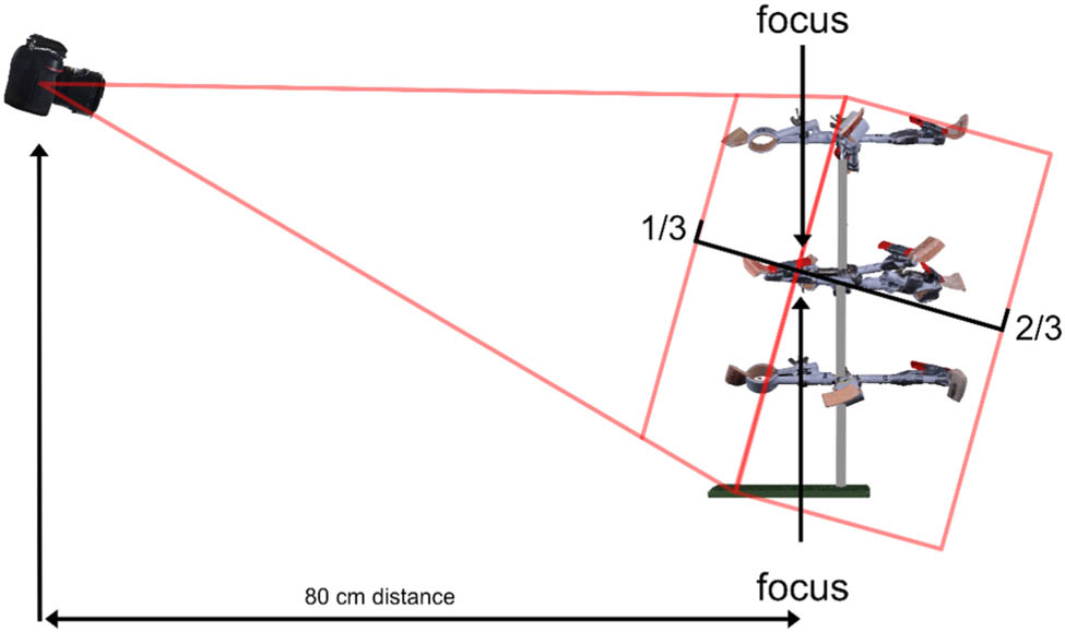
The dof depends on several factors consisting of distance (between point of focus and camera), aperture, used focal length, and camera geometry (sensor size and native aspect ratio). With our equipment (sensor: 35.9 × 23.9; native aspect ratio of 1.5:1; 35 mm focal length), a distance of 80 cm,^[13] and an aperture ratio of f/16, the dof measured 52.70 cm. If these parameters change, the dimensions of the dof change as well (Breuer et al., 2020, p. 54). Furthermore, the dof does not equally extend in both directions from the point of focus. The actual dimensions are roughly 2/3 of the dof ^[14] away from the point of focus and 1/3 of the dof toward the camera. If the focus is set on the “pottery tree,” all sherds will eventually be out of focus as soon as the rotation progresses. To avoid this, the focal point was moved towards the camera while maintaining an 80 cm distance between the camera and the pottery tree. This was done using a marker attached to a cylindrical bar magnet (ca. 5 cm length). The magnet can remain permanently attached and does not change in position, lowering variability. This marker was focused on via auto-focus, which was then disabled. Manual focus ensured that the dof remained static throughout an entire rotation (Figure 2).

However, if the camera’s angle is tilted, the angle of the dof changes simultaneously. Therefore, it is not always possible to have the lower and upper sherds inside the dof when using these steep angles (Figure 3).

Figure 2

Depiction of the depth of field and its relation to the pottery tree as well as the camera.

Figure 3

Depiction of the depth of field when the camera is tilted toward steeper angles.

If the blurring effect on these sherds is only marginal and limited to individual images, the processed surface geometry of the 3D model is not negatively affected. If this blurring effect becomes too large, surface geometry is heavily distorted leading to false measurements in the end.

Göttlich et al. (2021, Figure 9) used four angles in total. In smaller tests during the 2022 November campaign, we noticed that six or more angles did not necessarily improve the results but increased documentation time, storage necessity, and processing time. It was observed that fewer angles resulted in more false projections and insufficient overlap when the photography process started to become repetitive, and the concentration of the participants decreased. This might be worth to quantify for future projects to find the best balance between enough overlap or projection and low storage usage on the other side. To achieve a little more margin, lower the error rate, and generate more overlap between adjacent pictures along the vertical axis, we settled for five angles in total.

4 Interim Conclusion

As mentioned above, two stations (consisting of one “pottery tree,” one camera, and two people) were used for 18 workdays in the total campaign conducted in March 2022. During this time, one team tried to record as much data as possible in 1 day (7 h of work with a 1-h break and several shorter breaks in between) to see what was technically feasible. They managed to record 14 pottery trees.^[15] All trees were photographed carrying eight sherds, leading to an estimated maximum workload of 112 sherds per day. Since this entire process is highly repetitive, and working as fast as possible increased the probability of small mistakes due to lower concentration over time, we settled for organizing the work in a way that still provided a high output of images but did not overstrain the energy and concentration of the team. This resulted in a markedly lower error rate.^[16] Optimal results were achieved when photographing 8–10 trees per day and team (between 128 and 160 sherds documented daily).

Ultimately, only four people (two per station) documented more than 2,500 pottery sherds as 3D models in 18 full workdays (March 2022). This is significantly faster than drawing, involves fewer people, and leads to a much greater volume of accurate and precise documented sherds. Fifty-five additional pottery trees were documented in just 6 full workdays (November 2022), using ten clamps (ca. 550 sherds), while only two people did photography. This increased the output and did not decrease the quality of the models. Some tests were conducted using 12 clamps, which also did not affect the quality of the model.^[17] In 2023, only a team of three people serving two set-ups documented 1,264 sherds. Additionally, in all campaigns, we experienced regular power cuts, extending over periods of 4–5 h during both daytime and nighttime. However, our workflow was not affected by the temporary unavailability of electricity. Batteries for the camera, ring light, and remote control were charged overnight and completely charged during the few hours we had electricity. No difficulties for larger fragments were detected, including complete vessels^[18] (Figure 4).

Figure 4

3D model of a restored amphorae from Tell el-Burak using sfm.

Fragments below 15° of preservation were not documented with this methodology since their orientation (regardless of automatic or manual) is almost impossible to achieve precise and accurate values.^[19] Decorated pottery could be documented without altering the workflow^[20] including black-painted pottery such as Greek (Figure 5).

Figure 5

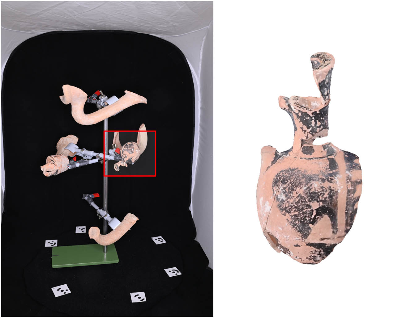
Black-painted pottery from Tell el-Burak on the pottery tree (left) and respective 3D model including calculated texture (right).

No completely black-painted sherds were included in this study. It is possible, however, that they interfere with the black background during the masking process which could be avoided by simply changing the background for a green or blue cloth.

5 3D Processing

Göttlich et al. (2021) used Agisoft Metashape (1.4.2) and MeshLab (V. 2016.12) for processing purposes. Pages 265–266 briefly describe the workflow in Agisoft. Images are loaded into Metashape, followed by the calculation of the sparse point cloud (high quality) and then the dense point cloud^[21] (high quality). Clamps are cut away from the dense point cloud. Marker distance is documented via so-called scale bars containing the respective distances measured between markers. The mesh is calculated in high quality. This is done for both passes of one pottery tree. Göttlich et al. (2021) exported both models and imported them into MeshLab to merge both models into one “whole” model without the holes created by cutting away the clamps. The merging was initially done using the open-source software MeshLab since Göttlich et al. (2021, p. 266) perceived the merging process in Metashape as unsatisfactory. Lastly, the model gets imported into Metashape again to calculate the respective texture.

In our study, we also decided to use Agisoft Metashape (V. 1.8.3). Other pay-to-use or open-source software is equally possible, but Metashape provides the most effective workflow and is more widely used throughout archaeology. It also offers the lowest price for pay-to-use software due to an educational license system.^[22] The instructions by Göttlich et al. (2021, pp. 265–266) were largely followed with minor changes. These changes will be addressed in the following text.

Göttlich et al. recorded photographs as RAW^[23] and converted them to JPEG (2021, Figure 10). We decided to convert RAW into TIFFs since this format provides far better quality and resolution. JPEGs are generally compressed,^[24] which lowers quality.^[25] Directly recording JPEG should be avoided altogether since, next to compression, JPEGs are systematically processed by the respective camera picture controls.^[26] This is not transparent because it is unclear which settings were used to process the images and alter parameters such as color, contrast, clarity, brightness, and saturation. The downside of this is larger storage necessities. With the used camera (Nikon D780 – 24.3 MP), individual file size averages at 26 MB (RAW) instead of 9 MB (JPEG). TIFFs are even larger, with an average of 150 MB per image. The latter, however, is only necessary for processing and can be deleted after the models are processed (see below). RAW files are kept for long-term storage. These files contain metadata such as camera settings and respective long-term storage strategies, following the FAIR principles, are implemented. In our case, the respective strategies are linked to the “Beyond Purple and Ivory Project” and will be presented in a separate publication together with additional data.

Identification of markers was done automatically using the detect targets function. The second step is to apply the camera calibration to correct any distortion produced by the lens construction and other distortion parameters rather than rely on manual calibration (see above). Metashape does this automatically due to the metadata embedded in the photograph from which the software can identify information such as the camera, lens, distance, aperture, shutter speed used, and so on. Since every camera position has individual distortion parameters, the pictures must be separated according to their respective angles. This not only improves overall quality but also lowers variability in results. The process is facilitated through the before-mentioned usage of different naming conventions and can be done via the camera calibration tool (BP1 = one group, BP2 = second group, etc.).

Masking remains heavily important since it reduces processing time drastically. However, it is not possible to simply use one picture as described by Göttlich et al. (2021, p. 266) because, without further editing, the projected mask remains static and does not rotate with the “pottery tree.” The photograph must first be imported into an image editing software, in our case “Paint.”^[27] The entire picture was selected and then deleted, leaving only the metadata embedded in the original file. If this “blank” image is then imported using the import mask and create mask from background settings, the mask will rotate correctly with every rotation of the tree for each photograph.

Singular points and additional noise can then be removed manually using the free-form selection tool. The result of a cleaned model is shown in Figure 6.

Figure 6

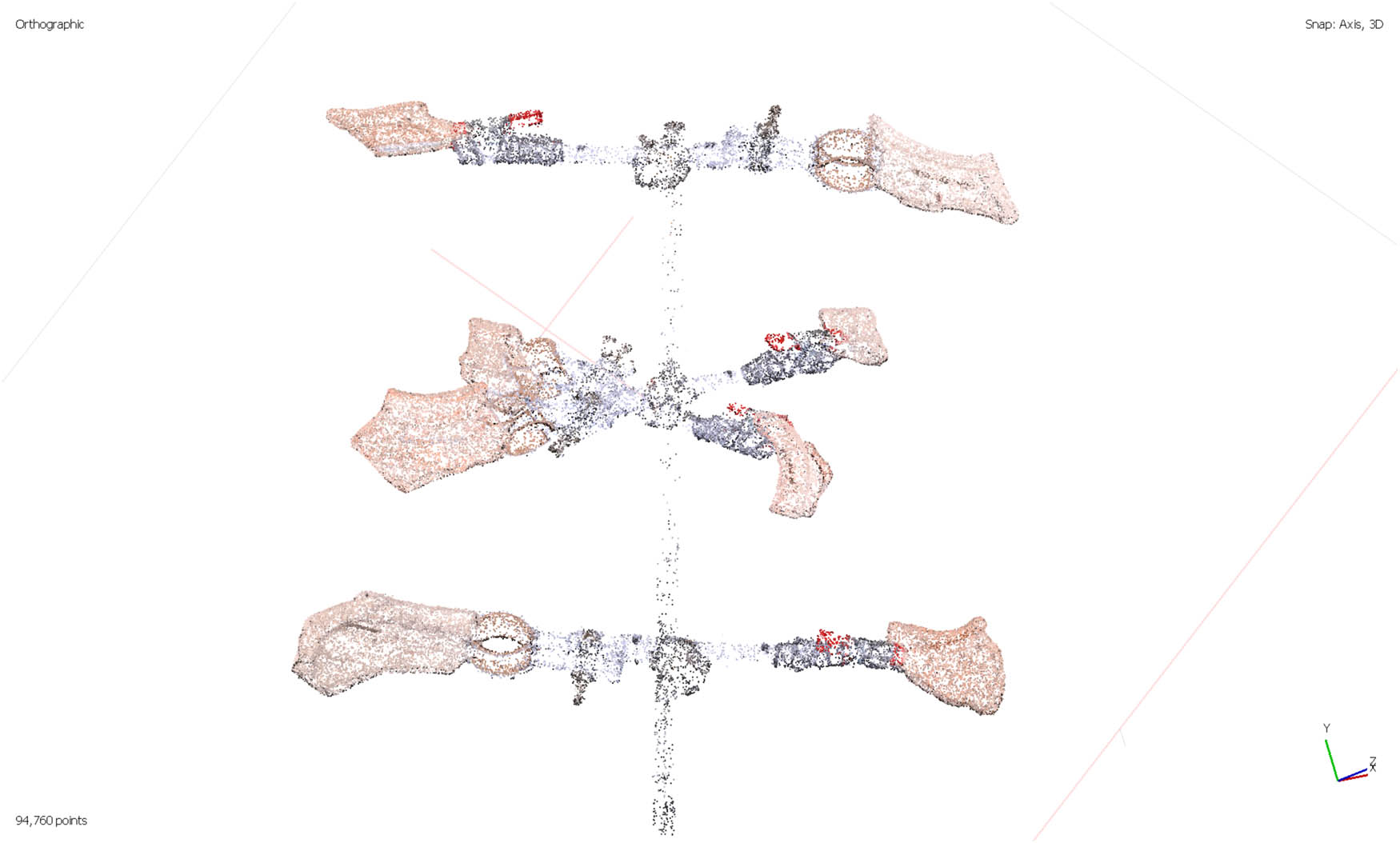
Depiction of the sparse-point cloud after removing unwanted noise.

Afterward, the sherds must be referenced, which is the most crucial aspect to achieve precise measurements of the sherds. This is done with the command create scale-bars (Göttlich et al., 2021, p. 265). After this step is completed, the optimize camera tool or the update button must be used to apply the referencing to the model.^[28]

Once the cleaning and referencing process is complete, the optimize cameras tool is used to recalculate the camera positions and apply the camera calibration, reducing error values such as error (pix).^[29] This is another aspect highly important in photogrammetry but not discussed by Göttlich et al. (2021). Ideally, the error values (error (pix)) are as low as possible since higher values necessarily mean higher levels of distortion. However, the gravity of this error depends on the measuring resolution, which was used to reference the models in the first place. Remember, our referencing included a ruler with 1 mm increments. Acceptable deviations are, therefore, ±0.5 mm (Taylor, 1982, pp. 8–9). In our case, models with values up to 3.0 error (pix) were still considered precise and accurate since deviations in mm equate to ca. 0.4 error (mm).^[30] This is below our maximum acceptable deviation, and manual measuring controls showed no significant deviations between the 3D model and the physical sherd.

The most significant difference between the article published by Göttlich et al. (2021) and the newly refined method described here is found in the order of the following steps: dense cloud calculation, creation of the mesh, and merging of models. Göttlich et al. calculated one dense cloud for the entire tree (2021, Figure 10), then separated each sherd into one chunk to process the meshes and merge models. We decided to split the sherds before calculating the dense cloud since unnecessary points (the entire structure of the pottery tree) do not have to be processed as well, which significantly lowers processing time. Dense cloud and mesh were calculated using the highest setting possible (“Ultra High Quality”) (Figure 7).

Figure 7

Depiction of the dense-point cloud and the calculated mesh.

Calculating the mesh only based on the depth maps is technically possible, which leaves out dense cloud processing and significantly lowers time. Dense cloud processing brought far better results in a direct comparison between mesh created from depth maps and dense clouds. Next to the fact that the mesh which is created via the depth maps is seriously distorted and less accurate, measurements show differences of 1 mm and are consequently above our considered error value of 0.5 mm (Figure 8). This is unfortunate since processing without dense cloud calculations is generally faster (see below). However, creating the mesh via depth map or dense cloud is subject to the desired resolution regarding measurements.

Figure 8

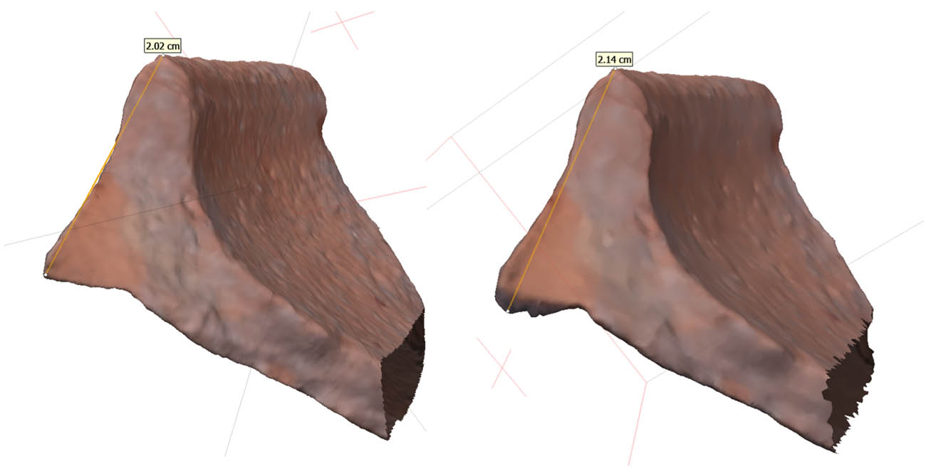
Comparison of two mesh processed via dense-cloud (left) and depth maps (right). Since the same sherd model is used, sherd orientation is based on the data used for referencing and is identical for both 3D models.

As mentioned above, the models are used to extract various additional measurements regarding the micro-morphometric characteristics of each sherd (thickness, diameter, rim thickness, inclination, etc.). Consequently, we are not interested in a complete reconstruction of the individual sherd for presentational aspects. Hence, it was decided not to merge sherds and calculate texture. However, by keeping all the raw data, this still remains an option and can easily be done again if needed. This reduces processing time significantly and allows us only to use one software rather than switching between Metashape and Meshlab, as proposed by Göttlich et al. (2021, p. 266). The clamp is removed from the model after the mesh is calculated in the highest setting possible. This leaves a hole in the sherd, but it did not affect automated measurements (Di Angelo et al., 2024). This is research specific and through the above-described documentation process on site (both pass-throughs photographed), merging remains an option. Marking the sherds with black dots – using a non-permanent marker – facilitates this significantly (Figure 9).

Figure 9

Depiction of the sherds carrying markings to facilitate the merging of models.

These points can be identified quickly on the images in Metashape and reduce the merging process from the original average of 30 min down to 5–10 min. Additionally, this eliminates the necessity of merging in MeshLab, and lengthy import/export situations can be avoided. Ultimately, the documented data support multiple analysis methods or research questions since all necessary information is stored in the raw material. It is therefore relatively easy and fast – without additional documentation time on site – to process selective models with texture or without holes by merging the models.

6 Interim Conclusion

Between 45 and 60 min of manual work is necessary to prepare and finish the results of one entire pottery tree.^[31] This is done without merging and texturing within the workflow described above. To be more precise, the whole process – from the moment images are imported into Metashape until the processing of the dense clouds – can be conducted in 45 min. After processing, 10 and 15 additional minutes are needed to remove noise from the dense clouds, choose the better pass of each sherd, cut away the clamps, and export the model. Exporting models can be done in a batch process using the “{chunklabel}” command.

The necessary time is usually reduced with increasing experience since the work is highly repetitive, and shortcuts and an efficient workflow heavily facilitate the process. Additionally, the required time only rises marginally if more clamps are put on the tree (between 5 and 10 min for each clamp). Processing time, on the other side, rises considerably but does not affect output since processing is done overnight. Additionally, through the background function, projects can easily be queued and processed one after the other. Certain aspects (alignment, masking, identifying targets, referencing) can again be automated via python scripts, reducing manual labor. All dense clouds are calculated in the highest setting possible (ultra-high). Our workstations^[32] need roughly 40 min to render one dense cloud of a model consisting of 9,000–15,000 points.^[33] Calculating all 16 chunks or dense clouds (Passes 1 and 2 of every sherd) takes, on average, 640 min (between 10 and 11 h), and is done overnight.

7 Discussion

Our results confirm that this method is fast, precise, accurate, and straightforward. Results can easily be shared and analyzed in depth. In terms of cost, this method is mainly seen as affordable or a “low-cost methodology” (Avella et al., 2015; Barreau et al., 2014; Göttlich et al., 2021, p. 256). This statement needs to be considered in relation to the respective research aim, especially when connected to the large-scale documentation of pottery. Cheaper equipment affects the results, and low- or mid-budget equipment will inevitably be less precise. It also limits the possibilities for high-quality resolution in the meshes, dense clouds, and textures. More affordable computers will need more time to process and render. On the other hand, high-quality equipment may result in better results or shorter render times but are more expensive. Especially with regard to high-end equipment, it seems this method raises financial costs compared to the traditional method of drawing. On the other hand, campaign time and needed people are lowered significantly, which again lowers cost.

Professional cameras that provide high-resolution images ( ≥ 24 MP) and contain a full-frame sensor can easily cost between 2,000 and 3,000€. Digital single-lens-mirrorless cameras (DSLM) can offer cheaper solutions, which still produce high-quality images and usually have a full-frame sensor.^[34] Additionally, DSLM cameras tend to be smaller and have less heavy weight, which facilitates traveling. Whether a team chooses DSLR or DSLM, one of the most important aspects is the necessity of including high-quality lenses, which are also expensive. On the other side, cheaper solutions can contribute to distortion and error parameters and negatively affect model quality.

Additional equipment includes tripods, remote switches, batteries, high-capacity SD cards, ring lights, a light tent, a turntable, external hard drives for backup, and the actual pottery tree. Furthermore, one or two adequate computers must be acquired, along with the necessary processing software. Additionally, it is necessary to consider indirect costs, such as hardware wear-and-tear and electricity consumption, as well as sufficient storage capacity for all the metadata produced. As mentioned above, one “pottery tree” equals roughly 10 Gb of RAW data. This requires large storage capacity provided via external hard drives or a cloud server, which adds to the overall expenses. The respective 3D files (.obj or .stl) measure between 5 and 20 Mb. Lastly, it has the potential to be conducted “low-cost” if cheaper equipment is used, but it barely can be considered to be truly “low-cost” as it rather shifts cost toward other expenses.

Ultimately, we reach the point where it is necessary to ask why one would document pottery solely as 3D models. In the following text, I will discuss the differences between traditional drawing, digital drawing, and 3D models.

First and foremost, drawings – regardless of whether they are traditionally or digitally drawn – are mainly done for presentational aspects only. They primarily serve the purpose of representation and aim to give the reader a clear overview of the form repertoire found in a specific site, region, or chronological period. This is important and has to be the basis of every analysis dealing with pottery, but it hardly exploits all potential embedded in this particular material culture. Creating a typology should not be the end of modern research projects but rather the starting point for more advanced analysis as observed by Vella (1996, p. 248).

It has been shown here and in other studies (Göttlich et al., 2021; Karasik & Smilansky, 2008; Wilczek et al., 2018) that documentation time is drastically reduced on-site, which lowers costs and minimizes the necessity for longer documentation campaigns. The 3D models cannot only be used to generate profile views, as presented by Göttlich et al. (2021), Karasik/Smilansky (2008), and Wilczek et al. (2018), but they contain all morphometric information of their physical counterparts.^[35] They can be analyzed extensively using advanced methodologies such as automated shape recognition, automated measurement analysis (Di Angelo et al., 2024), and other methods. Additionally, if pottery was documented as a 3D model, we could avoid losing – at least some – knowledge if future circumstances prohibit these sherds from being reexamined due to politically unstable situations or simply because the material culture is destroyed through the act of war. Consequently, far more information and knowledge of the respective material culture is documented through this methodology. Documenting with the LAP also reduces documentation time drastically since around 20–30 sherds per hour are easily possible. The result is a drawing although photographs are also possible to document surface treatment of sherds.^[36] All files are stored in an easy-to-use database system and can be altered or refined as well as shared effortlessly. However, it has to be recognized that results are not as extensive as 3D models. Lastly, this leads me to the next aspect that should be compared between all three methods: precision and accuracy.^[37]

It is possible to conduct measurements on certain variables (diameter, thickness, inclinations) on the physical sherd while drawing or on the drawing themselves. However, this can only be done on a portion – namely the profile – of the sherd. Consequently, measurements only reflect a specific part of the sherd and are more subject to bias if conducted on drawings or while drawing. For example, sherd orientation is done by hand (traditionally and with the LAP) and can vary individually based on the level of experience of the drawing person. This ultimately affects detected diameters, inclinations, and preservations and might distort results. With the LAP, diameter measurements are repeated n times, resulting in mean values and a standard deviation. This is quite helpful but depends on the time repeated measuring is conducted and on the correct and again manual orientation of the sherd during this measurement time.^[38] Highly reflective sherds such as stone vessels are in my experience rather difficult to document even with the respective settings for reflective surfaces. Regarding 3D models, orientation is done automatically using different algorithms or methodologies (Di Angelo et al., 2024; Karasik & Smilansky, 2008; Wilczek et al., 2018). Automated orientation as presented by Di Angelo et al. (2018) and Di Angelo et al. (2024) can of course still be subject to bias, however, would be biased continuously throughout the sample set – especially inside their respective subtypes. Consequently, a possible bias could be accounted for and – if identified – corrected.

Manual measurements of thickness are limited to certain areas of the sherd, and especially with the LAP, only a very thin and isolated fraction of the sherd is measured. Using 3D models helps since the distance between n-points on the sherd surface can be measured, resulting in mean values representing the individual sherd far better than individual measuring spots (Di Angelo et al., 2024). Altogether, measurements taken from 3D models can be considered more accurate and precise, while traditional or digital drawings can also of course be accurate but remain less precise.

Here, one might ask why this level of precision and accuracy is needed and I would argue that through this higher resolution regarding measurements, far-reaching research questions using advanced methodologies such as quantification can be answered based on the most neutral measurement values possible. This is frequently done as several studies (Blackman et al., 1993; Gandon et al., 2018, 2020; Harush et al., 2020; Roux, 2003) aim to observe production parameters behind the material culture, such as standardization, specialization, and ultimately organization of production (see above). As already mentioned, in my case, morphometric measurements are needed to statistically analyze (using MANOVA) the data for my PhD thesis on Phoenician tableware pottery. Detecting a significant difference between assemblages, types, or settlements based on morphometry, because the measurements are distorted or biased would be very problematic and misleading. Consequently, the documentation methodology for such an analysis needs to be highly reliable and to produce accurate and precise results in the shortest amount of time while documenting the required (larger) sample size. However, the necessary data can be collected as part of a sample from the excavated pottery. Consequently, not all pottery has to be documented as a 3D model.

It is obviously possible to create a computer-assisted drawing from a 3D model as presented by several studies (Göttlich et al., 2021; Karasik & Smilansky, 2008; Wilczek et al., 2018) but using the LAP for this is faster, cheaper and equally accurate. It is equally possible to use profile sections to measure morphometric vessel features to conduct quantitative analysis but results are less precise and potentially subject to an individual bias which distorts results as presented elsewhere (Di Angelo et al., 2024). Generally, it would be great to have 3D models for entire ceramic collections of any given excavation, but this remains not advisable right now, especially if one is only interested in an overview regarding the form repertoire found at a specific site. However, as mentioned above traditional and digital drawings as well as 3D models ultimately can serve different purposes and consequently, it has to be questioned if a constant comparison of the methods is even appropriate. Lastly, both methods produce different results from which different research questions can emerge.

In my opinion, the best solution would be to combine the method presented here with digital drawings provided through the LAP. The method presented here is best used to document a limited set of samples, which is intended to answer quantitative research questions that need this level of precision and accuracy. For such requirements, 3D modeling remains the best solution since all necessary information is embedded in the processed 3D model. It can be handled effortlessly while upholding the FAIR principles since the final result (the 3D model files) is rather small and can be uploaded on any database system. Documentation is fast, accurate, and precise; it can be done using only two people and in a very short amount of time in almost any surrounding, while the majority of excavated pottery can be documented through the LAP.

8 Conclusion

In this study, I presented a refined approach to the large-scale documentation of pottery using sfm based on the paper published by Göttlich et al. (2021). I provided detailed information regarding the workflow and technical details to make this methodology as reproducible as possible. This was further accompanied by the results of several case studies in which this methodology was truly tested in large-scale documentation surrounding. The results of ca. 2,500 fully documented pottery sherds in 18 full workdays show how fast this methodology is. Furthermore, this workflow is easy to learn if the right information is provided and produces reliable, accurate, and precise results. Time and cost spent on campaigns can be significantly reduced while the amount of documented sherds is high. However, this method is not low-cost effective because it has to be remembered that all models have to be processed off-site, and the respective infrastructure to process and save all the data is needed. This method is best conducted if a quantitative research approach is present and the analysis that needs this level of accuracy and precision can be conducted on a selected sample of pottery sherds. It is not advisable to simply document the entirety of pottery from an entire site. In this case, the costs would outweigh the benefits. A combined approach of using the LAP and this methodology is therefore proposed.

References

Agisoft LCC. (2021). Metashape Python Reference Release 1.8.0. https://www.agisoft.com/pdf/metashape_python_api_1_8_0.pdf.Search in Google Scholar
Avella, F., Sacco, V., Spatafora, F., Pezzini, E., & Siragusa, D. (2015). Low cost system for visualization and exhibition of pottery finds in archeological museums. SCIRES-IT - SCIentific RESearch and Information Technology, 5(2), 111–128. doi: 10.2423/i22394303v5n2p111.Search in Google Scholar
Barreau, J., Nicolas, T., Bruniaux, G., Petit, E., Petit, Q., Bernard, Y., Gaugne, R., & Gouranton, V. (2014). Ceramics fragments digitization by photogrammetry, reconstructions and applications. International Conference on Culturage Heritage. https://arxiv.org/abs/1412.1330.Search in Google Scholar
Blackman, M. J., Stein, G. J., & Vandiver, P. B. (1993). The standardization hypothesis and ceramic mass production: Technological compositional and metric indexes of craft specialization at Tell Leilan, Syria. American Anqituity, 58(1), 60–80.10.2307/281454Search in Google Scholar
Breuer, M., Czichon, R. M., Koch, M., Lehmann, M., & Mielke, D. P. (2020). Photogrammetrische 3D-Dokumentation von Nassholzfunden aus Oymaagac Höyük/Nerik (Provinz Samsun/TR). Restaurierung Und Archäologie, 2017(10), 47–62.Search in Google Scholar
Demján, P., Pavúk, P., & Roosevelt, C. H. (2022). Laser-Aided Profile Measurement and Cluster Analysis of Ceramic Shapes. Journal of Field Archaeology, 1–18. doi: 10.1080/00934690.2022.2128549.Search in Google Scholar
Di Angelo, L., Di Stefano, P., Guardiani, E., & Pane, C. (2020). Automatic shape feature recognition for ceramic finds. Journal on Computing and Cultural Heritage, 13(3), 1–21. doi: 10.1145/3386730.Search in Google Scholar
Di Angelo, L., Di Stefano, P., & Pane, C. (2018). An automatic method for pottery fragments analysis. Measurement, 128, 138–148. doi: 10.1016/j.measurement.2018.06.008.Search in Google Scholar
Di Angelo, L., Schmitt, A., Rummel, M., & Di Stefano, P. (2024). Automatic analysis of pottery sherds based on structure from motion scanning: The case of the Phoenician carinated-shoulder amphorae from Tell el-Burak (Lebanon). Journal of Cultural Heritage, 67, 336–351. doi: 10.1016/j.culher.2024.03.012.Search in Google Scholar
Gandon, E., Coyle, T., Bootsma, R. J., Roux, V., & Endler, J. (2018). Individuals among the pots: How do traditional ceramic shapes vary between potters? Ecological Psychology, 30(4), 299–313. doi: 10.1080/10407413.2018.1438200.Search in Google Scholar
Gandon, E., Nonaka, T., Endler, J. A., Coyle, T., & Bootsma, R. J. (2020). Traditional craftspeople are not copycats: Potter idiosyncrasies in vessel morphogenesis. PloS One, 15(9), 1-18. doi: 10.1371/journal.pone.0239362.Search in Google Scholar
Göttlich, F., Schmitt, A., Kilian, A., Gries, H., & Badreshany, K. (2021). A new method for the large-scale documentation of pottery sherds through simultaneous multiple 3D model capture using structure from motion: Phoenician carinated-shoulder amphorae from Tell el-Burak (Lebanon) as a case study. Open Archaeology, 7(1), 256–272. doi: 10.1515/opar-2020-0133.Search in Google Scholar
Green, S., Bevan, A., & Shapland, M. (2014). A comparative assessment of structure from motion methods for archaeological research. Journal of Archaeological Science, 46, 173–181. doi: 10.1016/j.jas.2014.02.030.Search in Google Scholar
Harush, O., Roux, V., Karasik, A., & Grosman, L. (2020). Social signatures in standardized ceramic production – A 3-D approach to ethnographic data. Journal of Anthropological Archaeology, 60, 101208. doi: 10.1016/j.jaa.2020.101208.Search in Google Scholar
Jones, C. A., & Church, E. (2020). Photogrammetry is for everyone: Structure-from-motion software user experiences in archaeology. Journal of Archaeological Science: Reports, 30, 102261. doi: 10.1016/j.jasrep.2020.102261.Search in Google Scholar
Karasik, A., & Smilansky, U. (2008). 3D scanning technology as a standard archaeological tool for pottery analysis: Practice and theory. Journal of Archaeological Science, 35(5), 1148–1168. doi: 10.1016/j.jas.2007.08.008.Search in Google Scholar
Newton, M. (2022). Full Frame vs APS-C – Image Quality is Key! https://www.theschoolofphotography.com/tutorials/full-frame-vs-aps-cSearch in Google Scholar
Rönnberg, M., Büyükyaka, M., Kamlah, J., Sader, H., & Schmitt, A. (2023). Preliminary report on the Cypriot and Greek imports from the Iron Age settlement at Tell el-Burak, Lebanon. A first survey of imported pottery reaching the Central Levant, ca. 750–325 BCE. Rivista Di Study Fenici, 51(51), 37–71. doi: 10.19282/rsf.51.2023.02.Search in Google Scholar
Roux, V. (2003). Ceramic standardization and intensity of production: Quantifying degrees of specialization. American Antiquity, 68(4), 768–782. doi: 10.2307/3557072.Search in Google Scholar
Schmitt, A., Badreshany, K., Tachatou, E., & Sader, H. (2019). Insights into the economic organization of the Phoenician homeland: A multi-disciplinary investigation of the later Iron Age II and Persian period Phoenician amphorae from Tell el-Burak. Levant, 50(1), 52–90. doi: 10.1080/00758914.2018.1547004.Search in Google Scholar
Sokal, R. R., & Rohlf, F. J. (2012). Biometry: The principles and practice of statistics in biological research (4th ed.). Freeman.Search in Google Scholar
Szeliski, R. (2022). Computer vision: Algorithms and applications (2nd ed.). Texts in computer science. Springer.10.1007/978-3-030-34372-9Search in Google Scholar
Taylor, J. R. (1982). An introduction to error analysis: The study of uncertainties in physical measurements. A series of books in physics. Univ. Science Books.Search in Google Scholar
VanPool, T. L., & Leonard, R. D. (2011). Quantitative analysis in archaeology (1. publ). Wiley-Blackwell.10.1002/9781444390155Search in Google Scholar
Vella, N. (1996). Elusive phoenicians. Antiquity, 70(268), 245–250. doi: 10.1017/S0003598X00083241.Search in Google Scholar
Waldhäusl, P., & Ogleby, C. (1994). 3-Rules for simple photogrammetric documentation of architecture. International Archives of Photogrammetry and Remote Sensing, 30, 426–429.Search in Google Scholar
Wilczek, J., Monna, F., Jébrane, A., Chazal, C. L., Navarro, N., Couette, S., & Smith, C. C. (2018). Computer-assisted orientation and drawing of archaeological pottery. Journal on Computing and Cultural Heritage, 11(4), 1–17. doi: 10.1145/3230672.Search in Google Scholar
© 2024 the author(s), published by De Gruyter
This work is licensed under the Creative Commons Attribution 4.0 International License.
Articles in the same Issue
- Regular Articles
- Social Organization, Intersections, and Interactions in Bronze Age Sardinia. Reading Settlement Patterns in the Area of Sarrala with the Contribution of Applied Sciences
- Creating World Views: Work-Expenditure Calculations for Funnel Beaker Megalithic Graves and Flint Axe Head Depositions in Northern Germany
- Plant Use and Cereal Cultivation Inferred from Integrated Archaeobotanical Analysis of an Ottoman Age Moat Sequence (Szigetvár, Hungary)
- Salt Production in Central Italy and Social Network Analysis Centrality Measures: An Exploratory Approach
- Archaeometric Study of Iron Age Pottery Production in Central Sicily: A Case of Technological Conservatism
- Dehesilla Cave Rock Paintings (Cádiz, Spain): Analysis and Contextualisation within the Prehistoric Art of the Southern Iberian Peninsula
- Reconciling Contradictory Archaeological Survey Data: A Case Study from Central Crete, Greece