An analytical method with Padé technique for solving of variational problems

H. Jaffarian; K. Sayevand; Sunil Kumar

doi:10.1515/nleng-2016-0065

Artikel Open Access

An analytical method with Padé technique for solving of variational problems

H. Jaffarian , K. Sayevand und Sunil Kumar

Veröffentlicht/Copyright: 6. September 2017

Veröffentlicht von

Veröffentlichen auch Sie bei De Gruyter Brill

Manuskript einreichen Informationen für Autor*innen

Aus der Zeitschrift Nonlinear Engineering Band 6 Heft 4

Abstract

In this paper, the homotopy analysis method (HAM) is employed to solve a class of variational problems (VPs). By using the so-called ħ-curves, we determine the convergence parameter ħ, which plays key role to control convergence of solution series. Also we use Pade’ approximant to improve accuracy of the method. Two test example are given to clarify the applicability and efficiency of the proposed method.

Keywords: Variational problems; Euler-Lagrange; Homotopy analysis method; Padé

MSC 2010: 41A58; 39A10; 34K28; 41A10

1 Introduction

1.1 Motivation of paper

The investigation of exact solutions to fractional VPs plays an important role in the study of nonlinear physical phenomena.

1.2 Some history

The Homotopy analysis method (HAM) has been presented by Liao [1, 2, 3], to obtain the analytical solutions for various nonlinear problems. There are many letters that deal with Homotopy analysis method such as, Abbasbandy et al. [4] applied the Newton-homotopy analysis method to solve nonlinear algebraic equations, Allan [5] constructed the analytical solutions to Lorenz system by the HAM, Bataineh et al. [6, 7] proposed a new reliable modification of the HAM, Alomari and et al. introduced the solution of delay differential equation by means of homotopy analysis method , Chen and Liu [9] applied the HAM to increase the ciatonvergent region of the harmonic balance method, Liao [10] proposed the HAM to study nonlinear problems and others [11, 12].

1.3 Structure of paper

In this paper, we extend the application of HAM for solving variational problems. The structure of this paper is organized as follows.

In Section 2, we present our main results concerning to our method. In Section 3, we present a test example. Finally, we end the paper with few concluding remarks in Section 4.

2 VPs with Caputo fractional derivative

Consider the following functional

Jy=∫abF(x.yx,y′(x))dx(1)

defined on the set of continuous curves y : [0, 1] → R, where F has continuous derivatives with respect to the second, third and fourth variable. Consider the problem of finding the extremum of the functional (1) with boundary conditions y (a) = A and y (b) = B. Let us denote this problem by (P). A necessary condition for problem (P) is given by the next theorem.

Theorem1

(see [12]) If y is a local minimizer to problem (P), then ysatisfies the Euler-Lagrange equation

∂F∂y−ddx∂F∂y′=0,ya=A,yb=B(2)

The Euler-Lagrange equation (2) is in general a nonlinear differential equation of fractional order, which does not always have an analytic solution.

3 Solution guidelines for variational problems

First, we rewrite the Euler-Lagrange equation in the following operator form

Lyx+Nyx−gx=0,ya=A,yb=B.(3)

where L is a linear operator, N is a nonlinear operator which contains differential operators less than 2 and g(x) is a given function.

Let ħ denote a nonzero auxiliary parameter. By means of generalizing the traditional homotopy method, we construct the so-called zero th-order deformation equation

1−pLYx;p−Y0x=pℏ[Lyx+N[yx]−gx]),(4)

Where pε[0, 1] is the so-called homotopy parameter, (x; p : [a, b] × [0, 1] → R, and Y₀ defines the initial approximation of the solution of (3). Assume the solution of (3) to be in the form

Y=Y0+pY1+p2Y2+p3Y3+…(5)

In order to determine the functions Y_j, j = 1, 2, 3, … substituting (5) into (4) and collecting terms of the same power of p gives

LY1=ℏLY0+N0Y0−gx,LY2=LY1+ℏ[LY1+N1[Y0,Y1]]LY3=LY2+ℏLY2+N0Y0,Y1,Y2,⋮

where

NY0+pY1+p2Y2+p3Y3+…=N0Y0+pN1Y0,Y1+P2N2Y0,Y1,Y2,

and

N0N1N2N3N4⋮=10000…0Y1000…0Y212!Y1200…0Y3Y1Y213!0…0Y412!Y22+Y1Y312!Y12Y214!Y14…⋮⋮⋮⋮⋮…N~[Y0]N′~[Y0]N″~[Y0]N(‴)~[Y0]N(4)~[Y0]⋮

where

N(n)~Y0=N(n)Y0+∑m=1∞Ympm|P=0,n=0,1,2,…

Then, the solution of (2) has the form

y(x)=limn→∞∑j=0nYjx.(6)

If it is difficult to determine the sum of series (6), then as an approximate solution of the equation, we approximate the solution y(x) by the truncated series

ynx=∑j=0nYjx.(7)

3.1 Convergence theorem

Theorem 1

(see [1]) If the solution series defined by (6) is convergent, then it must be the solution of the equation (2).

Theorem 2

(see [13]) Let A(ħ) be a continuous function on [a₁ , b₁]. Further, suppose that yⁿ (x, A(ħ)) be the approximate solution about A(ħ), then

∀ϵ>0,x¯ϵa1,b1,∃N0and∃ℏ1,ℏ2,sothat

∀ℏϵℏ1,ℏ2andn≥N0⇒yx¯,Aℏ−ynx¯,Aℏ<ϵ.(8)

Theorem 3

(see [13]) Let A(ħ) be a continuous function on [a₁ , b₁ ] and yⁿ (x, A(ħ)) be the series of (7) about A(ħ) such that for each fixed ħ is a function of x, then the curve of yⁿ (x, A(ħ)), where x ∊ (a₁ , b₁), becomes a horizontal line when n → ∞.

Theorem 4

(see [13]) Let A(ħ) be a continuous function on [a₁ , b₁ ] and yⁿ (x, A(ħ)) be the series of (7) about A(ħ) such that for each fixed ħ is a function of x, then the curve of ddxynx,Aℏ|x=x¯, where x ∊ (a₁ , b₁ ), becomes a horizontal line when n → ∞.

Remark

So, it can be deduced that if for every fixed x ∊ (a₁ , b₁ ), the ħ-curve becomes horizontal, thus the series (7) is convergent, and according to the Theorem 1, converges to the exact solution.

3.2 Padé technique

There exist some techniques to improve the convergence rate of a given series by HAM. Among these techniques, the so-called Padé technique is widely applied. The so-called homotopy- Padé technique was suggested by means of combining the Padé technique with HAM [1]. For a give series

Y=∑j=0∞yjpj,(9)

the corresponding [LM] Padé approximant is expressed by

LM=∑j=1Lripj1+∑j=1Mqjpj,(10)

The formal power series:

Y=∑j=0∞YjPj(11)

Y−∑j=0Lrjpj1+∑j=1Mqjpj=OpL+M+1,(12)

Determine the coefficients r_j and q_j by equating. Then, we can write out (12) in more details as:

YL+1+YLq1+…+YL−MqM=0,YL+2+YL+1q1+…+YL−M+2qM=0⋮YL+M+YL+M−1q1+…+YLqM=0(13)

Y0=r0Y1+Y0q1=r1⋮YL+YL−1q1+…+Y0qL=rL(14)

Setting p = 1 provides the [LM] Padé approximant

LM=YL−M+1…YL+1…⋱…YL…YL+M∑j=MLYj−M…∑j=0LYjYL−M+1…YL+1…⋱…YL…Yl+M1…∑j=0LYj(15)

For more details refer to [14].

4 Test examples

In this section, we solve a test problem to demonstrate the accurate nature of the proposed method. The validity of the method is based on assumption that the series (5) converges at q = 1. There is the convergence control parameter A(ħ) which guarantees that this assumption can be satisfied. We need to concentrate on the convergence of the obtained results by properly choosing ħ.

Example 1

Consider the problem of finding the minimum of the functional

Jy=∫011+y2(x)y′2(x)dx,(16)

with boundary conditions

y0=0,y1=0.5.(17)

The exact solution of this problem is y(x) = sinh(0.4812118250596x).

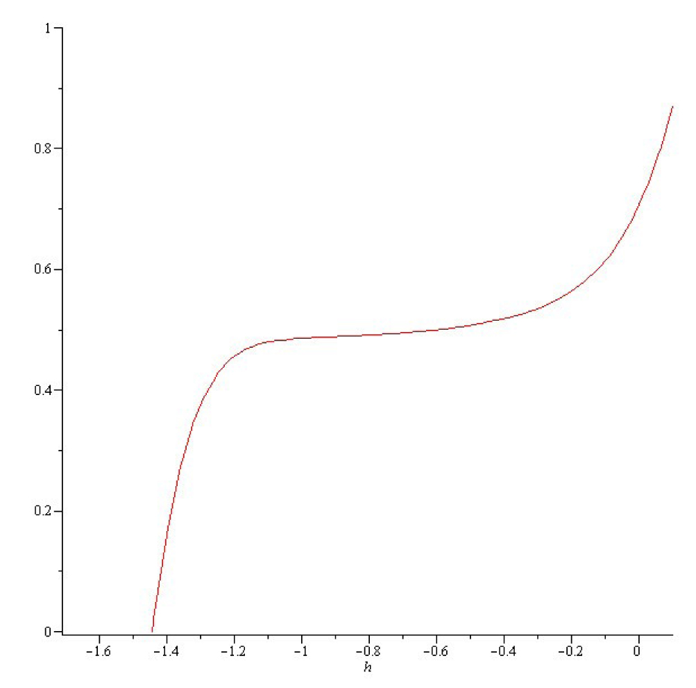
We choose y0(x)=π2 as initial approximation guess. We study the influence of ħ on the convergence of y¹⁰(1). We can investigate the influence of ħ on the convergence region of y¹⁰(1) by means of ħ -curve as shown in Fig. 1 From Fig. 1, the convergence region of y¹⁰(1) is [−1.2,−0.3]. The absolute values of the errors are given in Table 1 which proves the accuracy of the solution.

Fig. 1

The ħ -curve of y¹⁰(1).

Table 1

The absolute errors of the solutions for Example 1.

x	y_exact	ħ = −0.9	ħ = −0.5
0.1	0.0481397563	4.56E–6	5.98E–6
0.2	0.0963910086	5.60E–6	5.24E–6
0.3	0.1448655114	6.05E–6	6.23E–6
0.4	0.1936755370	8.76E–6	9.87E–6
0.5	0.2429341332	9.36E–6	1.56E–5
0.6	0.2927553881	6.14E–5	7.86E–5
0.7	0.3432546921	5.21E–5	6.12E–5
0.8	0.3945490069	4.77E–4	5.87E–4
0.9	0.4467571349	5.08E–4	7.43E–4

We employ the Padé technique to gain more accurate approximations of the solution, as shown in Table 2.

Table 2

The [LM] padé approximant for Example 1

x	66	77	[88]
0.1	0.0481399145	0.0481398235	0.0481398143
0.2	0.0963913376	0.0963912365	0.0963911255
0.3	0.1448658458	0.1448657355	0.1448656331
0.4	0.1936759781	0.1936758684	0.1936757566
0.5	0.2429344883	0.2429343784	0.2429332645
0.6	0.2927585751	0.2927574832	0.2927563297
0.7	0.3432578831	0.3432567985	0.3432557102
0.8	0.3945754189	0.3945653129	0.3945562789
0.9	0.4467995789	0.4467873909	0.4467772909

5 Concluding remarks

In this paper, we studied the application of the HAM for solving the variational problems. One advantage of this method is the use of a computational algorithm with fast convergence. We also used Padé approximant to improve accuracy of the HAM. An example is presented to illustrate the accuracy of the present method. The given example reveal that the HAM yields a very effective and convenient technique to the approximate solutions of the variational problems.

References

[1] S. J. Liao: Beyond Perturbation: Introduction to Homotopy Analysis Method, Chapman Hall/ CRC Press, Boca Raton (2003).10.1201/9780203491164Suche in Google Scholar

[2] S. Abbasbandy, Y. Tan and S. J. Liao: Newton-homotopy analysis method for nonlinear equations, Appl. Math. Comput. 188(2007) 1794-1800.10.1016/j.amc.2006.11.136Suche in Google Scholar

[3] S. Abbasbandy: Solitary wave solutions to the Kuramoto Sivashinsky equation by means of the homotopy analysis method, Nonlinear Dynam. 52 (2008) 35–40.10.1007/s11071-007-9255-9Suche in Google Scholar

[4] S. Abbasbandy and E.J. Parkes: Solitary smooth hump solutions of the Camassa-Holm equation by means of the homotopy analysis method, Chaos Solitons Fract. 36 (2008) 581–591.10.1016/j.chaos.2007.10.034Suche in Google Scholar

[5] F. M. Allan: Construction of analytic solution to chaotic dynamical systems using the Homotopy analysis method, Chaos Solitons Fractals 39(2009) 1744-1752.10.1016/j.chaos.2007.06.116Suche in Google Scholar

[6] A. S. Bataineh, M. S. M. Nooraniand and I. Hashim: Solving systems of ODEs by homotopy analysis method, Commun. Nonlinear Sci. Numer. Simul. 13(2008) 2060-2070.10.1016/j.cnsns.2007.05.026Suche in Google Scholar

[7] A. S. Bataineh, M. S. M. Noorani and I. Hashim: On a new reliable modifcation of homotopy analysis method, Commun. Nonlinear Sci. Numer. Simul. 14(2009) 409-423.10.1016/j.cnsns.2007.10.007Suche in Google Scholar

[8] A. K. Alomari, M. S. M. Noorani and R. Nazar: Solution of delay differential equation by means of homotopy analysis method, Acta. Appl. Math. 108(2009) 395-412.10.1007/s10440-008-9318-zSuche in Google Scholar

[9] Y. M. Chen and J. K. Liu: Improving convergence of incremental harmonic balance method using homotopy analysis method, Acta. Mech. Sin. 25(2009) 707-712.10.1007/s10409-009-0256-4Suche in Google Scholar

[10] S.J. Liao: The proposed homotopy analysis technique for the solution of nonlinear problems, PHD thesis, Shanghai Jiao Tong University (1992).Suche in Google Scholar

[11] S. J. Liao: An approximate solution technique not depending on small parameters: a special example, Int. J. Non-linear Mech. 30(1995) 371-380.10.1016/0020-7462(94)00054-ESuche in Google Scholar

[12] T. Odzijewicz, A. B. Malinowska and D. F. M. Torres: Fractional variational calculus with classical and combined Caputo derivatives, Nonlinear Anal . Theory Methods Appl. 75(3) (2012) 1507-1515.10.1016/j.na.2011.01.010Suche in Google Scholar

[13] M. Ghasemi, M. Fardi and R. K. Ghaziani: Solution of system of the mixed Volterra-Fredholm integral equations by an analytical method, Math. Comput. Model. 58(2013) 1522-1530.10.1016/j.mcm.2013.06.006Suche in Google Scholar

[14] G. A. Baker: Essentials of Padé approximants, Academic Press, London (1975).Suche in Google Scholar

Received: 2016-10-11

Accepted: 2017-7-6

Published Online: 2017-9-6

Published in Print: 2017-12-20

This article is distributed under the terms of the Creative Commons Attribution Non-Commercial License, which permits unrestricted non-commercial use, distribution, and reproduction in any medium, provided the original work is properly cited.

Artikel in diesem Heft

https://doi.org/10.1515/nleng-2016-0065

Schlagwörter für diesen Artikel

Variational problems; Euler-Lagrange; Homotopy analysis method; Padé

Creative Commons

BY-NC-ND 3.0