A New Computational Technique for the Generation of Optimised Aircraft Trajectories
-
Kenneth Chircop
 ,
David Zammit-Mangion
,
David Zammit-Mangion

Abstract
A new computational technique based on Pseudospectral Discretisation (PSD) and adaptive bisection ε-constraint methods is proposed to solve multi-objective aircraft trajectory optimisation problems formulated as nonlinear optimal control problems. This technique is applicable to a variety of next-generation avionics and Air Traffic Management (ATM) Decision Support Systems (DSS) for strategic and tactical replanning operations. These include the future Flight Management Systems (FMS) and the 4-Dimensional Trajectory (4DT) planning and intent negotiation/validation tools envisaged by SESAR and NextGen for a global implementation. In particular, after describing the PSD method, the adaptive bisection ε-constraint method is presented to allow an efficient solution of problems in which two or multiple performance indices are to be minimized simultaneously. Initial simulation case studies were performed adopting suitable aircraft dynamics models and addressing a classical vertical trajectory optimisation problem with two objectives simultaneously. Subsequently, a more advanced 4DT simulation case study is presented with a focus on representative ATM optimisation objectives in the Terminal Manoeuvring Area (TMA). The simulation results are analysed in-depth and corroborated by flight performance analysis, supporting the validity of the proposed computational techniques.
1 Introduction
Trajectory optimisation has been a core research topic in the aerospace engineering domain for several decades. Most of the operational, economic and environmental performances of an aerospace vehicle’s mission are in fact directly correlated to the flown trajectory [1]. The maximisation of range or endurance performances and the minimisation of fuel-based or time-based costs are some of the objectives that have been frequently pursued in these studies. In the 1930’s, Ernst Zermelo studied the problem of wind-optimal aircraft routing [2,3]. This was one of the first and most challenging trajectory optimisation problems tackled in the aerospace domain, extensively investigated by De Jong and the Royal Netherlands Meteorological Institute in the 1970’s [4], and is still actively researched at present [5–7]. While the steady-state approximations of aircraft dynamics adopted in these and more generic aircraft performance studies have been very successful in providing the rough figures required to develop Multidisciplinary Design Optimisation (MDO) and basic flight planning algorithms, the limitations of this approach have been increasingly evident with the steady growth of air traffic, which has resulted in new constraints on route and airspeed and in an increasing congestion in low altitude terminal airspace regions. To resolve the emerging issues and simultaneously improve the predictability of traffic demand, the aviation research community has committed to better capture aircraft, airspace and airport dynamics in all trajectory planning, prediction and management algorithms that will be integrated in future avionics and Air Traffic Management (ATM) Decision Support Systems (DSS). This evolution will be enabled by shifting from legacy flight plans to 4-Dimensional Trajectory (4DT) intents which will be exchanged, negotiated and updated continuously by exploiting Air-to-ground Data-Links (ADL) communications [8–11].
When introducing aircraft dynamics in the problem statement, the formulation of the Trajectory Optimisation Problem (TOP) mathematically corresponds to the formulation of the Optimal Control Problem (OCP). Optimal control is exploited for a wide range of engineering problems, as it permits finding theoretically optimal control laws that minimise a performance criterion (cost functional) of a dynamic system through mathematical optimisation techniques. In the aerospace and avionics domain, the optimisation process involves defining aircraft dynamics, path costraints (imposed by adverse weather conditions or by ATM and Air Traffic Flow Management services) and a set of objectives (usually formulated to maximise fuel/time efficency and to reduce the environmental impacts) to compute trajectories that are optimal with respect to user-preferred performances. The aircraft dynamics model consists of a set of differential equations correlating the system states and its control inputs, which are usually accompanied by a set of constraints on the control inputs leading to a reduced set of admissible inputs or controls. The solution of the OCP consists in determining the admissible inputs that fulfill all constraints and, in doing so, minimize the cost functional [12]. The techniques available to solve aerospace OCP are reviewed in [13–16]. Traditionally, OCP were solved using indirect methods, applying the calculus of variations or Pontryagin’s maximum principle to satisfy first-order necessary conditions for optimality [13–16]. These methods are characterized by attempting an explicit solution of the optimality conditions stated in terms of the adjoint differential equations, the maximum principle, and associated boundary conditions [14]. This is practical for classical problems and some special weakly non-linear low dimensional systems. However, to obtain a solution of dynamic systems described by strongly non-linear differential equations, it is necessary to use numerical methods [13]. These methods suffer from the fact that the addition of new constraints requires deriving new necessary conditions. In many complex problems, determining the necessary conditions in a useful form can be a very difficult task [26]. As problems became more complex, indirect methods became increasingly harder to use, eventually being replaced by the more computationally intensive direct methods. Direct methods transcribe the continuous OCP into a parameter optimisation problem [8910111213141516]. Satisfaction of the system equations is accomplished by integrating them stepwise using either implicit or explicit rules; in either case, the effect is to generate non-linear constraint equations which must be satisfied by the parameters, which typically correspond to the discretised state and control histories [27]. The problem is thus converted from the original infinite dimensional OCP into a finite Non-Linear Programming (NLP) problem that can be solved using standard NLP solvers. A significant opportunity is recently identified when considering the application of very efficient direct numerical OCP solution methods for aircraft 4DT planning and management algorithms [1]. Visser, among others, analysed the application of OCP in 4D Trajectory Based Operations (TBO) [8]. Since the concept of 4D-TBO by itself required substantial research, the subsequent Programme for Harmonised ATM Research in EUROCONTROL (PHARE) research initiative focussed on the operational concept [17–19]. With the growing concerns for environmental sustainability of aviation in the last decade, the application of optimal control to compute environmentally optimal aircraft trajectories has been one of the key focus subjects of the Systems for Green Operations Integrated Technology Demonstrator (SGO-ITD) of the Clean Sky joint technology initiative for aeronautics and air transport [1,20–22]. As part of this and similar endeavours, a need for more versatile multi-objective formulations, encompassing operational, economic and environmental criteria at the same time was identified [23]. Although a large number of studies have tackled the application of optimal control techniques to aircraft flight trajectories, only a few have undertaken such investigation with the aim of implementing these aspects in avionics and ATM DSS [23]. A notable challenge consists in the transposition of the mathematically opimal trajectory computed by OCP solution methods into an operationally meaningful 4DT that can be flown by state-of-the-art Automated Flight Control Systems (AFCS) and that can be concisely described so to minimise the impacts on the data-link bandwidth and system processing [24]. Due to the aforementioned growing focus in multi-objective TOP formulations, computationally efficient bi- and multi-objective optimality techniques are an essential element of 4DT optimisation algorithms that will be integrated in future avionics and ATM DSS. The work presented in this paper investigates the adoption of custom developed techniques to solve aircraft TOP using direct methods to determine optimal trajectories. The computationally-efficient adaptive bisection ε-constraint scalarisation method is adapted to attain a computationally-efficient generation of Pareto frontiers for bi-objective optimal control problems (BOOCPs). This method is well suited for bi- and multi-objective trajectory optimisation algorithms that will be implemented in future avionics and ATM DSS. The underlying NLP solver which is used for the solution of the discretised BOOCP is the open-source large-scale non-linear solver IPOPT [28], which has been integrated with the MATLAB environment , where all the algorithms were numerically verified in representative simulation case studies. The basis of this work was initially presented in [30].
The paper is structured as follows. Section 2 formulates a generic single-objective continuous OCP that is discretised using pseudospectral techniques in Section 3. In Section 4, the discretised OCP is transcribed into a parameter optimisation problem that can be supplied to the NLP solver. In Section 5, the OCP is extended to encompass bi-objective problems, and the formulation of the adaptive bi-section ε-constrained scalarisation method is described in Section 6, supporting an efficient solution of bi-objective TOP with standard solvers. Section 7 discusses the NLP solver selection and its implementation in our algorithms. In Section 8, the techniques are validated against a classical problem of optimal control theory (i.e., the brachistochrone). Furthermore, a conventional vertical trajectory optimisation problem is evaluated. Section 9 presents the proposed implementation of these algorithms to solve realistic single- and multi-objective 4DT optimisation problems in avionics and ATM DSS for 4D-TBO. The paper terminates with some concluding remarks and directions for further research.
2 Optimal control problem formulation
In general, a Single-Objective Optimal Control Problem (SOOCP) is solved by finding the state trajectories x(t), the control trajectories u(t), and times t0 and tf in the interval t ∈ [t0,tf], that minimize a specific cost functional J. The problem is formulated as follows [31]:
where ϕ is the endpoint cost and L is the integrand cost, known as the Mayer and Lagrange cost respectively. The SOOCP is subjected to the following constraints that must be satisfied by the solution:
where ẋ represents the system dynamics in the form of differential constraints, and h and e are the path and event constraints respectively. The state, control and time variables are also bounded as follows:
3 Pseudospectral discretisation
Solving the OCP analytically is generally very difficult even for simple problems and becomes prohibitive for complex nonlinear problems. This difficulty can be eliminated adopting efficient numerical techniques on digital computers. By following this approach, the OCP is discretised such that state and control trajectories are represented by vectors of discrete values for each time interval. The solution of the resulting discretised OCP involves a number of steps, the most computationally intensive of which are those approximating the derivatives of the state trajectories at the discretisation nodes and integrating the cost functionals. Over the last few years, pseudospectral discretisation techniques have emerged as the most effective transcription methods for solving complex nonlinear OCP owing to their accuracy and speed, with an impressive convergence rate known as spectral accuracy [32]. In particular, for smooth problems, spectral accuracy implies an exponential convergence rate [33]. For these reasons, pseudospectral techniques are now very commonly adopted in aerospace TOP and have been selected for this work. The pseudospectral formulation starts with a polynomial expansion, which is well known in numerical analysis [34]. If τ0τ1,…,τN are N + 1 distinct values and f is a function whose values are given at those values, then a unique polynomial P(τ ) of degree at most N exists with:
Assume that {pk}k = 0,1,… is a system of algebraic polynomials (with degree of pk = k) that are mutually orthogonal over the interval (–1, 1) with respect to a weight function w ≠ 0 [35]:
The classical Weierstrass theorem implies that such a system is complete in the space
The formal series of a function
where the coefficients of the expansion are given by:
Equation 13 represents the polynomial transform of f. For an integer N > 0, the truncated series of f of order N is the polynomial:
The polynomial P(τ)in equation 10 is known as a Lagrange polynomial and it is given by:
where
A particular class of orthogonal polynomials are the Legendre polynomials. The Legendre polynomials Lk (τ), k = 0, 1, …, N are the eigenfunctions of the singular Sturm-Liouville problem. If Lk (τ) is normalised (i.e., Lk (1) = 1) then for any k:
where [k/2] denotes the integral part of k/2. Consider the N-th degree Legendre orthogonal polynomial LN(τ). The polynomial LN has N – 1 extrema τk, i.e.,
is exact for all polynomials p of degree ≤ 2N – 1. Legendre Gauss, Legendre-Gauss-Radau and Legendre-Gauss-Lobatto (LGL) series are the most common Legendre series, the choice of which determines the relative displacement of the quadrature nodes and their corresponding weights. Since equations for the quadrature nodes are not available in explicit form, the associated values have to be calculated using implicit numerical approximations. The quadrature weights can be expressed in closed form in terms of the nodes, as indicated in the following formulas for the LGL series, which is used extensively in the literature for trajectory optimisation:
If L(τ) is a general smooth function, then for a suitable N, its integral over τ ∊ [–1, 1] can be approximated as follows:
In a collocation method the fundamental representation of a smooth function f on τ ∊ [–1, 1] is in terms of its values at the discrete Gauss-type points. Derivatives of the function are approximated by analytic derivatives of the interpolating polynomial. The interpolating polynomial is denoted by IN f and satisfies:
Since it is a polynomial of degree N, interpolated over the LGL nodes as a discrete expansion using Legendre polynomials, funtion f admits an expression of the form:
Therefore, from equation 14, the weights of the expansion are approximated as follows:
where
Since IN f (τ) is an interpolant of f (τ) at the LGL nodes, and since the interpolating polynomial is unique, IN f (τ) may be expressed as a Lagrange interpolating polynomial:
so that equations 24 and 27 are mathematically equivalent. It is possible to write the Lagrange basis (or characteristic) polynomials as follows:
The use of polynomial interpolation to approximate a function using the LGL points is known in the literature as the Legendre pseudospectral approximation method. Denote f N (τ)=IN f (τ). Then,
It should be noted that Lk (τj) = 1 if k = j and Lk (τj) = 0, if k ≠ j, so that:
If the function f is known at the LGL quadrature points, one can compute an approximate derivative of f by differentiating the interpolant IN f and evaluating it at the same nodes. The polynomial of degree N – 1
is called the Legendre interpolation derivative of f relative to the chosen set of quadrature nodes, since in general, it is different from the projection derivative
The entries (DN) kl can be computed by differentiating the characteristic Lagrange polynomials Lk of degree N, which are 1 at τl and 0 at all the other collocation points. For the commonly used Gauss-Lobatto points, the closed form for the first-derivative matrix is:
The discretisation process of the general OCP derived in Section 2 commences with the introduction of the following transformation [36]:
This results in the mapping:
The objective of the OCP solution process is now to find the state and control trajectories x(τ) and u(τ) respectively, in the interval τ ∈ [–1, 1], and times t0 and tf, which minimize the performance index:
subject to the following constraints and bounds:
In the Legendre pseudospectral approximation, the state and control trajectories x(τ) and u(τ) respectively, in the interval τ ∈ [–1, 1], are approximated by Nth order Lagrange polynomials xN(τ) and uN(τ) based on interpolation at the Legendre-Gauss-Lobatto nodes [33]:
where xN(τ) and uN(τ) are the Lagrange interpolating polynomials, and ϕk(τ) are known as Lagrange basis polynomials. It should be noted that ϕk (τj) = 1 if k = j and ϕk (τj) = 0 if k ≠ j such that:
The derivative of the state vector is approximated as follows:
where D is (N + 1) × (N + 1) differentiation matrix corresponding to the LGL nodes. By defining uNand xN as the nu × (N + 1) control and nx × (N +1 ) state matrices storing the trajectories at the LGL nodes respectively:
Then, the trajectory of the state derivatives can be easily calculated with a simple matrix multiplication such that ẋN = xNDT to result in the ẋN matrix of dimensions nx × (N + 1):
The matrix of the differential constraints, i.e. the RHS of the differential equations in the OCP formulation, of dimensions nx × (N + 1) is calculated at each node as follows:
The matrix of differential defects at the collocation points, of dimensions nx × (N + 1), is obtained from the subtraction of the differential constraints from the state derivatives:
The differential defects are introduced to enforce the differential constraints at the LGL nodes. A subsequent step consists in defining the matrix of path constraint function values evaluated at the LGL nodes as:
The objective function of the OCP is therefore approximated as follows:
where the weights ωk are defined at the LGL nodes.
4 NLP formulation
In Non-linear Programming (NLP), a feasible solution of a system of equalities and/or inequalities is determined over a set of unknown variables, such that an objective function is minimized. In general, a NLP problem is defined as:
where y is the vector of decision variables of size ny to be optimised with lower and upper bounds yli and yui respectively. gj (y) and hk (y) are the r inequality and s equality constraints respectively. The OCP can be directly transcribed into a NLP problem by following a simple procedure. The objective function can be derived directly from equation (55), by constructing the decision vector y as a combination of the state vector xN, the control vector uN and the initial and final times t0 and tf respectively. This results in vector y having dimension ny = nx(N + 1) + nu(N + 1) + 2 and this can be expressed as:
The decision vector is constrained by a lower bound vector yli and an upper bound vector yui:
The equality constraint vector hk (y) is constructed from the differential constraints such that:
with the dimension of the equality constraints vector r equal to nx(N + 1). The equality constraints vector incorporates the path, event and time constraints with their respective bounds:
5 Generic BOOCP problem formulation
In aircraft trajectory optimisation, it is often the case that flight planners as well as aircraft designers and operators need to determine the optimal control law that minimizes the fuel consumption and the time of flight, or a compromise might be required between carbon dioxide and nitrogen oxides emissions. These are inherently BOOCPs. In the bi-objective case, the OCP is formulated similarly to the SOOCP in Section 2 with the exception for equation (1) which is now modified to cater of two objective functions:
where i = 1,2.
Following the pseudospectral discretisation and approximation processes described in Section 3, the objective functions are calculated as follows:
where i = 1,2. NLP formulation of the BOOCP will lead to the following problem:
Solving the BOOCP problem results in a Pareto set of optimal solutions. A standard NLP solver is limited to solving only single objective optimisation problems. Therefore, a scalarisation technique (also known as multi-objective articulation of preference techniques) needs to be used to reduce the BOOCP into a series of SOOCPs to populate the Pareto frontier. The three most applied scalarisation methods in the literature are the linear weighted sum (LWS), the normal boundary intersection (NBI) and the normal constraint (NC) methods. In previous works, the authors of this paper have proposed a new method, that of the adaptive bisection ε-constraint method which has been shown to perform better than the reviewed methods [30,37]. Hence, the adaptive bisection ε-constraint method was adopted to generate Pareto frontiers for the BOOCPs in this work.
6 Adaptive bisection ε-constraint method
The adaptive bisection ε-constraint method [37], is a scalarisation method conceived to efficiently generate optimal Pareto frontiers in BOOCPs. Similarly to other scalarisation methods, the Pareto frontier is generated by solving a sequence of single-objective optimisation problems in a systematic manner. In this method, one of the objective functions is selected to be optimised while the other is converted into an additional constraint, leading to a solution that can be proven to always be weakly Pareto optimal. Systematic modifications to the value of the objective function forming the additional constraint leads to the generation of an evenly distributed Pareto frontier. The method transforms the BOOCP into np SOOCPs, where np is user specified and it determines the target number of points on the Pareto frontier. The algorithm starts by obtaining the anchor points
with the additional constraint:
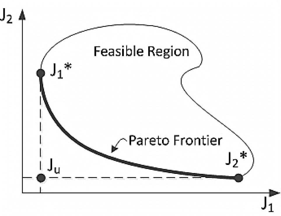
Graphical representation of the design metric space of a BOOCP.
The value of εc for each of the remaining SOOCPs is calculated as follows. Once the the anchor points are determined, the utopian line, which is a straight line joining the anchor points, is bisected to obtain the first value of εc in equation (75). The solution of the resulting SOOCP will lead to an additional point on the Pareto frontier. Sometimes this will lead to an infeasible problem that leads to no solution. In this case, the line joining the anchor points is subdivided into four sections and the constraint εc is set to the value of J2 at one-fourth the length of the line. If the problem is still infeasible, the value of J2 at three-quarters of the line joining the anchor points is then tried. The line will continue being bisected until a solution is found or a constant K set by the user is reached. Once an additional point
7 NLP solver implementation
A number of Nonlinear Programming solvers are publicly available, the predominant ones are SNOPT, IPOPT and fmincon. SNOPT is a software package for solving large-scale optimisation problems (linear and nonlinear programs) that was developed by Gill, Murray and Saunder [38]. It is implemented in Fortran 77 and distributed as source code against a license fee. IPOPT is an interior-point optimiser that was written by Wächter to solve large-scale nonlinear optimisation problems [39]. The algorithm is written in C++ and distributed open-source. Finally, fmincon is a function included in MATLAB’s optimisation toolbox which seeks the minimiser of a scalar function of multiple variables, with a region specified by linear constraints and bounds. In this work, both IPOPT and fmincon were adopted to demonstrate that the proposed method is non-solver-specific, as the intended application to avionics and ATM DSS will require the impementation in potentially very diverse platforms, such as ADA language on 64bit Acorn RISC Machine (ARM64) architectures. SNOPT was not used due to software licensing restrictions. The trajectory optimisation tool can be configured to use either fmincon or IPOPT. However, the latter is the preferred solver because in all test cases, IPOPT always converged faster than fmincon or converged in cases when fmincon did not find a solution. The execution time depends significantly on the length and complexity of the required trajectory.
8 Vertical trajectory optimisation case studiy
An aircraft trajectory optimisation problem was tackled to demonstrate the validity of the presented technique. The trajectory optimisation problem involves generating a Pareto frontier of optimal climb trajectories for an aircraft flying from 35 ft Above Mean Sea Level (AMSL) to a cruising altitude of 35,000 ft AMSL while covering a range of 900 kilometres. Two cost functionals were considered in this case: the minimization of flight time and the minimization of fuel consumption. Eurocontrol’s Base of Aircraft Data (BADA) coefficients of an Airbus A320 airliner were used to develop the aircraft dynamics model, following the methodology of Glover and Lygeros [41], described by the following state equations:
where X is the horizontal distance (range) covered by the aircraft on the ground, h is the altitude AMSL , V is the true airspeed (TAS) of the aircraft and m is the mass of the aircraft. X, h, V and m constitute the four state variables characterising the vertical profile of the aircraft. The control inputs are the flight path angle y, and the thrust ratio TR, which is a fraction of the maximum thrust available from the engines at a particular altitude, Tmax. The engine model integrated in the set of dynamic constraint to determine Tmax as a function of altitude and airspeed is an empirical turbofan thrust model adopted by BADA. CD is the coefficient of drag that varies with the aircraft configuration i.e. take-off, initial climb or clean. S represents the total area of the lifting surfaces on the aircraft, ρ is the air density at a particular value of h assuming standard atmospheric conditions and f is the rate of fuel consumption. Finally, g is the gravitational acceleration assumed to be constant. The initial and final conditions of the aircraft, formulated as event constraints in the BOOCP problem are defined in Table 1. Representative path constraints were applied to the trajectory optimisation problem to reproduce realistic limits on the performance of the aircraft and its propulsion system. The first path constraint is the stall speed of the aircraft which is a function of the aircraft configuration and constitutes the minimum value for the airspeed. The upper end of the speed scale is limited by VMO and MMO which are the maximum operating speed and the maximum operating Mach number respectively. Finally, the maximum thrust provided by the engines is also formulated as a path constraint.
BOOCP event constraints.
| Event | Initial or Final Condition |
|---|---|
| 1 | Xi = 0 km |
| 2 | hi = 35 ft |
| 3 | Vi = 165.2 kts |
| 4 | mi = 68 tonnes |
| 5 | Xf = 900 km |
| 6 | hf = FL 350 |
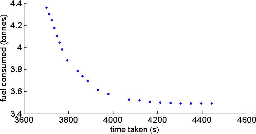
The Pareto frontier of this climb case study is presented in Figure 2. The frontier is evenly distributed and illustrates the extremal solutions at the far ends of the frontier, as well as intermediate solutions that provide a compromise between fuel consumed and flight time for a particular trajectory. The altitude-range profiles of the complete Pareto set are illustrated in Figure 3 as a three-dimensional surface plot. The trajectory at the front of the surface is the minimum time trajectory, whereas the profile at the far back represents the trajectory which consumes the least fuel. The complete surface is filled with successive plotting of trajectories representing the rest of the points in the Pareto optimal set. The discussion henceforth will focus on the extremal solutions.
Pareto frontier for minimum time and minimum fuel burn.
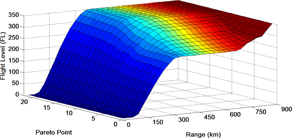
Altitude profiles for Pareto set.
Figure 4 illustrates the altitude-range profile for the two extremal solutions. A total of 4.36 tonnes of fuel are consumed in the minimum time trajectory, which is flown in 1 hr 2 mins. On the other hand, 3.49 tonnes of fuel and a flight time of 1 hr 14 mins characterise the minimum fuel trajectory. This means that for this specific problem, an increased flight time of 12 mins over a 900 km leg can be traded for approximately 20% of the fuel consumed.
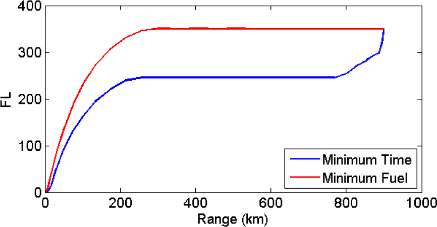
Altitude profile for minimum time and minimum fuel burn.
The minimum fuel trajectory involves a direct climb to the cruising altitude at which the aircraft flies the rest of the leg. This behaviour is expected since modern jetliners are most efficient at high altitudes where the air density is lower, which results in less drag on the aircraft. However, it is worth noting that the upper bound on the altitude in the BOOCP formulation was that of 45,000 ft giving the aircraft the possibility to fly higher than 35,000 ft in the level flight phase followed by a descent to the requested altitude at the end of the leg. This did not materialise, however, since the cost of attaining higher altitudes was larger than the savings in fuel yielded by flying a few flight levels higher. It is interesting to note that the minimum time trajectory follows a completely different strategy. The flight starts with a slightly shallower climb up to around 24,500 ft, followed by a level flight and finally an additional shallower climb to the requested altitude of 35,000 ft. The altitude flown for most of the time by the aircraft is the cross-over altitude i.e. the altitude at which the airspeed corresponding to the maximum operating Mach number MMO coincides with the maximum operating speed VMO. Consequently, this happens to be the altitude at which the aircraft can fly at the maximum true airspeed, which results in minimum flight time. In both cases, the climb from 35 ft occurs at the maximum thrust provided by the engine as can be seen in Figure 5. In the minimum time trajectory it is clear that engine thrust is kept at the maximum level permissible by operational constraints to gain the maximum possible airspeed which will result in minimal flight time. When minimising fuel costs, however, this is less obvious because fuel consumption is directly related to thrust levels. Reducing the thrust during the climb while keeping a constant flight path angle will result in a decrease in the rate of climb. As a result, it will take longer to reach the target altitude. Since the total fuel consumed during the climb is the integral of the rate of fuel consumption for the duration of the trajectory, the longer the flight time, the larger the fuel consumption. The optimisation results suggest that in the absence of winds it is more convenient to climb at high thrust levels (and high rates of fuel consumption) at high rates of climb rather than by simply keeping low thrust levels for a prolonged time. This is also understandable in the context that, for a given calibrated airspeed (CAS), TAS increases disproportionately with altitude. In still air, such as the case considered, TAS is what defines the ground speed and hence the flight time. As a result, it is expected that in the absence of winds it will be always advantageous to expedite climb in order to reach higher altitudes quicker.
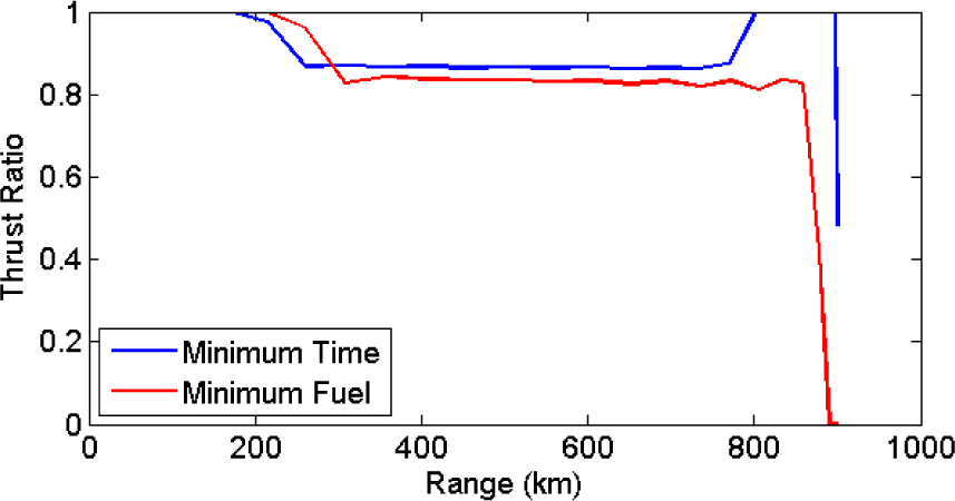
Thrust ratio profile for minimum time and minimum fuel burn.
The true airspeed and flight path angle (FPA) profiles illustrated in Figures 6 and 7 correlate perfectly with the observations previously made. The minimum time trajectory yields a speed profile that is larger in magnitude throughout the whole flight range over the minimum fuel counterpart. The former adopts a TAS of 495 kts, equivalent to 0.86 Mach, at the crossover altitude, while the latter flies at a nearly constant TAS varying from 419 kts to 410 kts at 35,000 ft. This result is consistent with the fact that during cruise, the aircraft would be expected to climb or slow down gradually as the aircraft becomes lighter through progressive fuel burn. In this case, the latter strategy was adopted. The steep climb of the minimum fuel trajectory is reflected in Figure 7 in which a maximum FPA of 6.2° is adopted as opposed to a maximum FPA of 4.4° in the minimum time case. The minimum time trajectory exhibits a lower climb gradient than its counterpart in order to afford a quicker TAS during the climb, since in both cases the engine thrust is set to the maximum level. Furthermore, in the minimum time trajectory, the second climb at the end of the trajectory, which is shallower than the first with a maximum FPA of 1°, is explained by the fact that at higher altitudes turbine engines generate less thrust due to the thinner atmosphere. Moreover, no trade-off is occurring between kinetic and potential energy to provide the additional rate of climb until the very end of the flight.
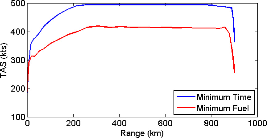
True Airspeed profile for minimum time and minimum fuel burn.
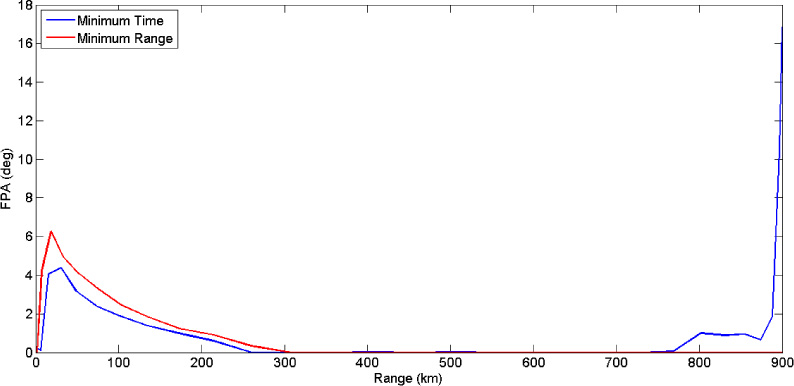
Flight path angle profile for minimum time and minimum fuel burn.
In Figures 5 to 7, it can be observed that the end of the trajectory is salient. In particular, in the minimum time profile the last 5,000 ft are climbed in just 12 km. Clearly, this is not practical for both operational and safety reasons. The speed profile during this time indicates a rapid decrease in TAS from 495 kts to 363 kts. The speed change occurs due to the trading of kinetic energy (speed) with potential energy (altitude), which is operationally defined zoom-climb [43], and also due to a rapid reduction in the thrust ratio. This zoom-climb solution falls within the feasible search space of the optimiser since no final condition is set on the speed in the problem formulation. A similar but less extreme shift is adopted in the minimum fuel trajectory. In this case, the aircraft is already flying at the cruise altitude at fuel-optimal speed. Since fuel consumption is of primary importance, in the final part of the trajectory the thrust is reduced to zero to conserve fuel leaving the aircraft to decelerate slowly towards the stall speed due to the aerodynamic drag. Theoretically this is possible since no constraints are included in the problem formulation even though for practical reasons such a solution is not operationally practical.
9 Combined later and vertical trajectory optimisation case study
As mentioned in section 1, the potential benefits of implementing trajectory optimisation techniques in avionics and ATM systems has recently met a growing interest by the research community. This case study therefore addresses the online planning of optimal 4DT intents in representative ATM scenarios. In particular, the spacing of dense arrival traffic towards in the Terminal Manoeuvring Area (TMA) was evaluated as a representative case study of online tactical 4DT planning. For trajectory optimisation of medium-large transport aircraft, Three Degrees of Freedom (3-DOF) point-mass aircraft dynamics are very commonly adopted. The 3-DOF implemented in our simulation case study is
where the state vector consists of: longitudinal velocity v [m s–1], flight path angle y [rad]; track angle 𝒳 [rad]; geographic latitude ϕ [rad]; geographic longitude λ [rad]; altitude z [m]; thrust angle of attack ∊ [rad]; aircraft mass m [kg]; and the control vector includes: thrust force T [N]; load factor N [ ]; bank angle μ [rad]. Other variables and parameters include: aircraft weight W and aerodynamic drag D [N]; wind velocity vw in its three scalar components [m s–1]; gravitational acceleration g [m s–2]; Earth radius RE [m]; fuel flow FF [kg s–1]. For turbofan aircraft, the following empirical expressions were adopted in the development of Eurocontrol’s Base of Aircraft Data (BADA), to determine the climb thrust and the fuel flow FF, which operationally equates to the maximum thrust TMAX in all flight phases excluding take-off [41]:
where τ is the throttle control, HP is the geopotential pressure altitude in feet, ΔT is the deviation from the standard atmosphere temperature in kelvin, vTAS is the true airspeed. CT1… CT5, Cf1… Cf4 are the empirical thrust and fuel flow coefficients, which are also supplied as part of BADA for a considerable number of currently operating aircraft [41]. While carbon dioxide (CO2) emissions are characterised by an approximately constant emission index of EICO2 = 3.16 [Kg/Kg], an empirical model for carbon monoxide (CO) and unburned hydrocarbons (HC) emission indexes (EICO/HC) in [g/Kg] at mean sea level based on nonlinear fit of experimental data from the ICAO emissions databank is:
where the fitting parameters c1,2, 3 accounting for the average emissions of 165 currently operated civil turbofan engines are c = {0.556, 10.208, 4.068} for CO and c = {0.083, 13.202, 1.967} for HC [23]. The nitrogen oxides (NOX) emission index [g/Kg] based on the curve fitting of 177 currently operated civil aircraft engines is [23]:
In the AMAN scenario, a best arrival sequence is defined by suitable scheduling algorithms. Longitudinal separation is enforced at the final approach fix to ensure sufficient separation upon landing and to prevent separation infringements in the approach phase itself. The assumed minimum longitudinal separation is 4 nmi on the approach path for medium category aircraft approaching at 140 knots, therefore the generated time slots are characterized by a 90~160 seconds separation depending on the wake-turbulence categories of two consecutive aircraft. The pseudospectral trajectory optimisation algorithm is therefore executed targeting a minimum fuel. The results of one representative simulation run are depicted in Fig. 8.
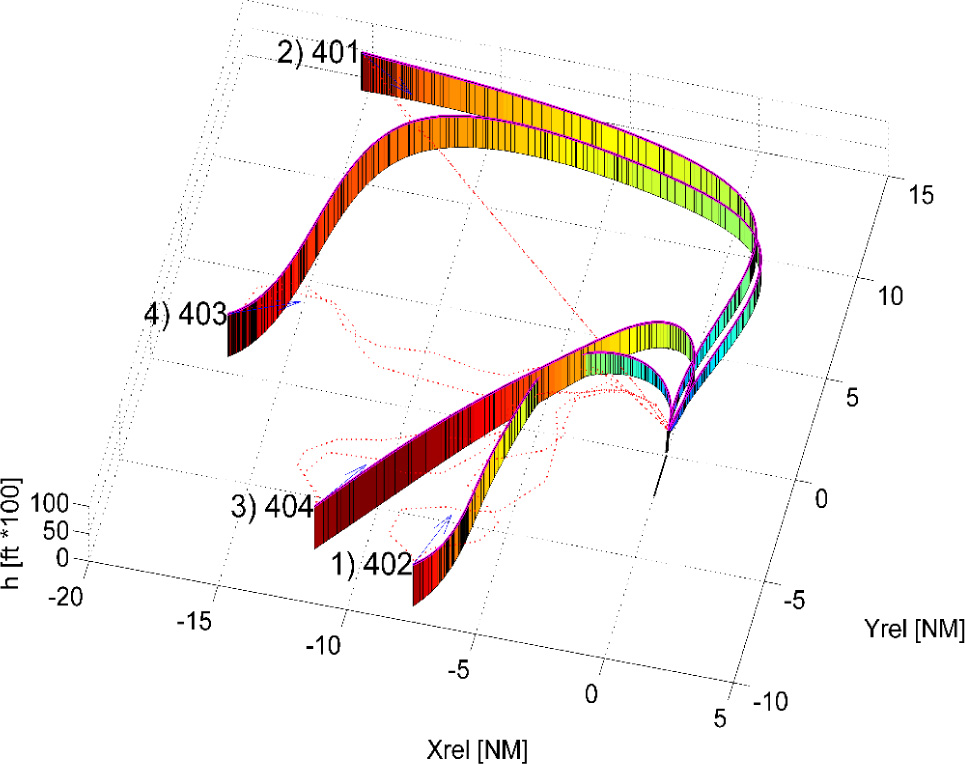
Results of the pseudospectral 4D trajectory optimisation algorithm applied to the online TMA trajectory planning scenario.
Computation times consistently below 20 seconds were achieved by our simulated ATM system to plan each 4DT intent of approximately 40 nmi with multiple path constraints in a representative TMA arrival and departure traffic conditions. Validated 4DT intents for multiple conflicting arrival traffic in a complex AMAN Terminal Sequencing and Spacing (TSS) scenario were produced in an average time of 41 seconds and consistently less than 60 seconds in a Monte Carlo simulation [25].
10 Conclusion and future work
This paper has presented a new computational technique to solve multi-objective aircraft trajectory optimisation problems formulated as optimal control problems. Due to their computational efficiency, pseudospectral methods were implemented to transcribe the formulated nonlinear optimal control problem. In terms of multi-objective optimality, the adaptive bisection ε-constraint scalarisation method was adopted to yield a very efficient generation of Pareto frontiers for a variety of bi- and multi-objective aircraft trajectory optimisation problems that are being currently investigated as part ofmajor aviation modernisation programmes. This multi-objective technique demostrates the required computational efficiency for implementation into avionics and Air Traffic Management (ATM) systems to generate optimal 4-Dimensional Trajectories (4DT) addressing multiple operational, economic and environmental criteria. A bi-objective vertical flight trajectory optimisation case study was evaluated in detail, involving a climb from 35 ft to a cruise altitude of 35,000 feet covering a range of 900 km and including operationally representative path constraints in terms of airspeed and engine thrust. The strategies adopted by the optimisation process are consistent with flight performance theory, therefore validating the algorithm. In particular, to maximise fuel efficiency in the absence of winds it is preferable to attain the cruise flight level as early as possible. Conversely, for maximised time performance it is preferable to interrupt the climb and maintain the crossover altitude as long as possible, then exploit the excess in kinetic energy to quickly reach the final cruise altitude. The proposed computational technique was also applied to the optimisation of 4DT intents in realistic ATM contexts. This work forms the basis of a trajectory optimisation tool that will be used to solve more complex and challenging problems in the future. The ultimate goal of the ongoing research is to develop innovative real-time trajectory optimisation methods which have the potential to be used in the next generations of ATM 4DT intent planning/negotiation systems and avionics Flight Management Systems (FMS). Trajectory optimisation algorithms based on pseudospectral discretisation and efficient Non-Linear Programming (NLP) solvers also have the potential to meet the real-time performance requirements for emergency avoidance such as in the case of obstacle warning systems and Sense-and-Avoid (SAA) systems [44–46]. Ongoing research activities are investigating the feasibility of avionics/ATM technologies capable of contributing to the emissions reduction targets set by ICAO and by European, American and Australian governments. In this respect, significant opportunities are emerging in relation with the adoption of multiobjective optimal control-based algorithms for trajectory planning and management considering multiple operational, economic and environmental criteria.
References
[1] Sabatini R, Gardi A, Ramasamy S, Kistan T, and Marino M, “Modern Avionics and ATM Systems for Green Operations”, in Encyclopedia of Aerospace Engineering, ch. eae1064, R. Blockley and W. Shyy, Eds., John Wiley & Sons, 2015.10.1002/9780470686652.eae1064Search in Google Scholar
[2] Zermelo E, “On navigation in the air as a problem in the calculus of variations (orig. Über die Navigation in der Luft als Problem der Variationsrechnung)“, Jahresbericht der Deutschen Mathematiker-Vereinigung, vol. 39, pp. 44-48, 1930.Search in Google Scholar
[3] Zermelo E, ”On the navigation problem for a calm or variable wind distribution (orig. Über das Navigationsproblem bei ruhender oder veränderlicher Windverteilung)“, Zeitschrift für Angewandte Mathematik und Mechanik, vol. 11, pp. 114-124, 1931.10.1002/zamm.19310110205Search in Google Scholar
[4] De Jong HM, “Optimal track selection and 3-dimensional flight planning - Theory and practice of the optimization problem in air navigation under space-time varying meteorological conditions”, Royal Netherlands Meteorological Institute (K.N.M.I.) 93, De Bilt, Netherlands, 1974.Search in Google Scholar
[5] Bijlsma SJ, “Optimal aircraft routing in general wind fields”, Journal of Guidance, Control, and Dynamics, vol. 32, pp. 1025-1028, 2009.10.2514/1.42425Search in Google Scholar
[6] Girardet B, Lapasset L, Delahaye D, and Rabut C, “Wind-optimal path planning: Application to aircraft trajectories”, 2014 13th International Conference on Control Automation Robotics and Vision, ICARCV 2014, 2014, pp. 1403-1408.10.1109/ICARCV.2014.7064521Search in Google Scholar
[7] Rodionova O, Sbihi M, Delahaye D, and Mongeau M, “North atlantic aircraft trajectory optimization”, IEEE Transactions on Intelligent Transportation Systems, vol. 15, pp. 2202–2212, 2014.10.1109/TITS.2014.2312315Search in Google Scholar
[8] Visser HG, “A 4D Trajectory Optimization and Guidance Technique for Terminal Area Traffic Management”, Delft University of Technology, 1994.Search in Google Scholar
[9] “The ATM Target Concept - D3”, SESAR Definition Phase DLM-0612-001-02-00, 2007.Search in Google Scholar
[10] “ATM Global Environment Efficiency Goals for 2050”, Civil Air Navigation Services Organisation (CANSO), 2012.Search in Google Scholar
[11] “European ATM Master Plan - The Roadmap for Sustainable Air Traffic Management”, SESAR JU, Brussels, Belgium, 2012.Search in Google Scholar
[12] Khan, S., Flight Trajectories Optimisation, 23rd Congress of the International Council of the Aeronautical Sciences (ICAS), Toronto, Canada, September, 2002.Search in Google Scholar
[13] Stryk, O. and Bulirsch, R., Direct and indirect methods for trajectory optimisation, Annals of Operations Research, vol. 37, no. 1, pp. 357–373, 1992.10.1007/BF02071065Search in Google Scholar
[14] Betts, J. T., Survey of numerical methods for trajectory optimisation, Journal of Guidance, Control, and Dynamics, vol. 21, no. 2, pp. 193–207, March-April 1998.10.2514/2.4231Search in Google Scholar
[15] Ben-Asher JZ, Optimal Control Theory with Aerospace Applications, Education Series, American Institute of Aeronautics and Astronautics (AIAA), Reston, VA, USA, 2010.10.2514/4.867347Search in Google Scholar
[16] Rao AV, “Survey of Numerical Methods for Optimal Control”, Advances in the Astronautical Sciences, vol. 135, pp. 497–528, 2010.Search in Google Scholar
[17] Wilson IAB, “PHARE: Definition and use of Tubes”, Programme for Harmonised Air Traffic Management Research in EUROCONTROL (PHARE), Brussels, Belgium, 1996.Search in Google Scholar
[18] Wilson IAB, “Trajectory Negotiation in a Multi-sector Environment”, Programme for Harmonised Air Traffic Management Research in EUROCONTROL (PHARE), Bruxelles, Belgium, 1998.Search in Google Scholar
[19] Fairclough I and McKeever D, “PHARE Advanced Tools - Trajectory Predictor - Final Report”, European Organisation for the Safety of Air Navigation (EUROCONTROL) DOC 98-70-18, Bruxelles, Belgium, 2000.Search in Google Scholar
[20] Camilleri W, Chircop K, Zammit-Mangion D, Sabatini R, and Sethi V, “Design and validation of a detailed aircraft performance model for trajectory optimization”, AIAA Modeling and Simulation Technologies Conference 2012 (MST 2012), Minneapolis, MN, USA, 2012.10.2514/6.2012-4566Search in Google Scholar
[21] Celis C, Sethi V, Zammit-Mangion D, Singh R, and Pilidis P, “Theoretical optimal trajectories for reducing the environmental impact of commercial aircraft operations”, Journal of Aerospace Technology and Management, vol. 6, pp. 29-42, 2014.10.5028/jatm.v6i1.288Search in Google Scholar
[22] Pisani D, Zammit-Mangion D, and Sabatini R, “City-pair trajectory optimization in the presence of winds using the GATAC framework”, AIAA Guidance, Navigation, and Control Conference (GNC 2013), Boston, MA, USA, 2013.10.2514/6.2013-4970Search in Google Scholar
[23] Gardi A, Sabatini R, and Ramasamy S, “Multi-objective optimisation of aircraft flight trajectories in the ATM and avionics context”, Progress in Aerospace Sciences, vol. 83, pp. 1–36, 2016.10.1016/j.paerosci.2015.11.006Search in Google Scholar
[24] Gardi A, Sabatini R, Kistan T, Lim Y, and Ramasamy S, “4-Dimensional Trajectory Functionalities for Air Traffic Management Systems”, IEEE/AIAA Integrated Communication, Navigation and Surveillance Conference (ICNS 2015), Herndon, VA, USA, 2015.10.1109/ICNSURV.2015.7121246Search in Google Scholar
[25] Gardi A., Ramasamy S., Sabatini R., and de Ridder K., “4-Dimensional Trajectory Negotiation and Validation System for the Next Generation Air Traffic Management”, AIAA Guidance, Navigation, and Control Conference (GNC 2013), Boston, MA, USA, 2013. 10.2514/6.2013-4893Search in Google Scholar
[26] Betts, J. T., Campbell, S. L. and Engelsone, A., Direct transcription solution of inequality constrained optimal control problems, Proceeding of the 2004 American Control Conference, Boston, Massachusetts, June 30 - July 2, 2004.10.23919/ACC.2004.1386809Search in Google Scholar
[27] Conway, B. A., A Survey of Methods Available for the Numerical Optimisation of Continuous Dynamic Systems, Journal of Optimisation Theory and Applications, vol. 152, no. 2, pp. 271–306, 2012.10.1007/s10957-011-9918-zSearch in Google Scholar
[28] Wächter, A. and Biegler L. T., On the Implementation of a Primal-Dual Interior Point Filter Line Search Algorithm for Large-Scale Nonlinear Programming, Journal of Mathematical Programming, vol. 106, no. 1, pp. 25–57, 2006.10.1007/s10107-004-0559-ySearch in Google Scholar
[29] MATLAB version 7.11. Natick, Massachusetts: The Mathworks Inc., 2010.Search in Google Scholar
[30] Chircop, K., Zammit-Mangion, D. and Sabatini, R. Bi-objective Pseudospectral Optimal Control Techniques for Aircraft Trajectory Optimisation, 28th Congress of the International Council of the Aeronautical Sciences, 23–28 September 2012.Search in Google Scholar
[31] Betts, J. T., Practical methods for optimal control using non-linear programming. SIAM: Philadelphia, PA, 2001.Search in Google Scholar
[32] Trefethen, L. N., Spectral Methods in MATLAB. SIAM, Philadelphia, PA, 2000.10.1137/1.9780898719598Search in Google Scholar
[33] Ross, I. and Fahroo, F., Legendre pseudospectral approximations of optimal control problems, Nonlinear Dynamics and Control and their Applications, vol. 295, pp. 327–342, 2004.10.1007/978-3-540-45056-6_21Search in Google Scholar
[34] Burden R. L. and Faires J. D., Numerical Analysis. Thomson Brooks/Cole, 2005.Search in Google Scholar
[35] Canuto C., Hussaini M. Y., Quarteroni A., and Zang T. A., Spectral Methods, Fundamentals in Single Domains. Springer-Verlag, 2006.10.1007/978-3-540-30726-6Search in Google Scholar
[36] Gill, P. E., Murray, W. and Wright, M. H., Practical Optimisation. Academic Press Inc: San Diego, CA, 1987.Search in Google Scholar
[37] Chircop, K. and Zammit-Mangion, D., On ε-constraint based methods for the generation of Pareto frontiers, Journal of Mechanics Engineering and Automation, vol. 3, no. 5, pp. 279–289.Search in Google Scholar
[38] Gill P. E., Murray W., and Saunders M. A., “User’s Guide for SNOPT Version 7,” pp. 1–116, 2008.Search in Google Scholar
[39] Wächter A., An interior point algorithm for large-scale nonlinear optimisation with applications in process engineering, 2002.Search in Google Scholar
[40] Ross I. M., A Primer on Pontryagin’s Principle in Optimal Control. Carmel, CA: Collegiate Publishers, 2009.Search in Google Scholar
[41] “User Manual for the Base of Aircraft Data (BADA) Revision 3.11”, Eurocontrol Experimental Centre (EEC) Technical/Scientific Report No. 13/04/16-01, Brétigny-sur-Orge, France, 2013.Search in Google Scholar
[42] Glover, W. and Lygeros, J., A Multi-Aircraft Model for Conflict Detection and Resolution Algorithm Evaluation, Technical Report WP1, Deliverable D1.3, Version 1.3, HYBRIDGE, February 18, 2004.Search in Google Scholar
[43] Pamadi BN, Performance, stability, dynamics and control of airplanes, AIAA Education Series, 2nd ed., American Institute of Aeronautics and Astronautics Inc. (AIAA), Blacksburg, VA, USA, 2004.Search in Google Scholar
[44] Sabatini R., Gardi A., Ramasamy S., and Richardson M. A., “A Laser Obstacle Warning and Avoidance System for Manned and Unmanned Aircraft”, 2014 IEEE International Workshop on Metrology for Aerospace, MetroAeroSpace 2014 proceedings, Benevento, Italy, 2014, pp. 616–621. 10.1109/MetroAeroSpace.2014.6865998Search in Google Scholar
[45] Sabatini R., Gardi A., and Ramasamy S., “A Laser Obstacle Warning and Avoidance System for Unmanned Aircraft Sense-and-Avoid”, Applied Mechanics and Materials, vol. 629, pp. 355–360, 2014. 10.4028/www.scientific.net/AMM.629.355Search in Google Scholar
[46] Ramasamy, S. and Sabatini, R., “A Unified Approach to Cooperative and Non-Cooperative Sense-and-Avoid”, 2015 International Conference on Unmanned Aircraft Systems (ICUAS ’15), Denver, CO, USA, 2015.10.1109/ICUAS.2015.7152360Search in Google Scholar
© 2016 Walter de Gruyter GmbH, Berlin/Boston
This article is distributed under the terms of the Creative Commons Attribution Non-Commercial License, which permits unrestricted non-commercial use, distribution, and reproduction in any medium, provided the original work is properly cited.
Articles in the same Issue
- Frontmatter
- A New Computational Technique for the Generation of Optimised Aircraft Trajectories
- Modelling of Imbibition Phenomena in Fluid Flow through Heterogeneous Inclined Porous Media with different porous materials
- Double dispersion effects on non-Darcy free convective boundary layer flow of a nanofluid over vertical frustum of a cone with convective boundary condition
- F1 style MGU-H applied to the turbocharger of a gasoline hybrid electric passenger car
- Nonlinear control systems - A brief overview of historical and recent advances
- An analytical method with Padé technique for solving of variational problems
- Influence of Lorentz force, Cattaneo-Christov heat flux and viscous dissipation on the flow of micropolar fluid past a nonlinear convective stretching vertical surface