Sensing with quantum light: a perspective
-
Animesh Datta


Abstract
I present my perspective on sensing with quantum light. I summarise the motivations and methodology for identifying quantum enhancements in sensing over a classical sensor. In the real world, this enhancement will be a constant factor and not increase with the size of the quantum probe as is often advertised. I use a limited survey of interferometry, microscopy and spectroscopy to extract the vital challenges that must be faced to realise tangible enhancements in sensing with quantum light.
1 Introduction
Over the ages, light has been central to sensing and detecting phenomena in the Natural world across length and timescales, from observational cosmology to nanoscopy. Light also happens to be the medium whose quantum properties are most readily redolent in ambient conditions [1]. Thus, it is only natural that sensing with quantum light has been investigated [2] and pursued with some vigour over the last decade [3], [4], [5], [6], [7], [8], [9], [10], [11]. It has enabled us to see things that would have been impossible without it [12].
My endeavour in this perspective on sensing with quantum light is to note some past advances and future challenges. Rather than a review, I aim to identify the underlying commonalities – in existing methodology and foreseeable problems. My choice of material is evidently selective. I focus on the three sensing modalities of interferometry, microscopy and spectroscopy. I choose them because they form large classes of sensing applications classically and have the potential of benefitting from quantum light. They also encapsulate amongst themselves the vital aspects of the principle and practice of sensing with quantum light and are naturally amenable to nanophotonics.
I begin with the mathematical formalism that captures sensing in Section 2. It presents the classical and quantum Fisher information as quantities to be evaluated to begin the process of identifying a quantum enhancement in sensing. I summarise its conceptual message – of identifying quantum enhancement due to quantum light over classical light in Figure 1. Establishing tangible enhancement of sensing quantum light can only be done experimentally. In Section 3, I encapsulate our understanding of classical and quantum light.
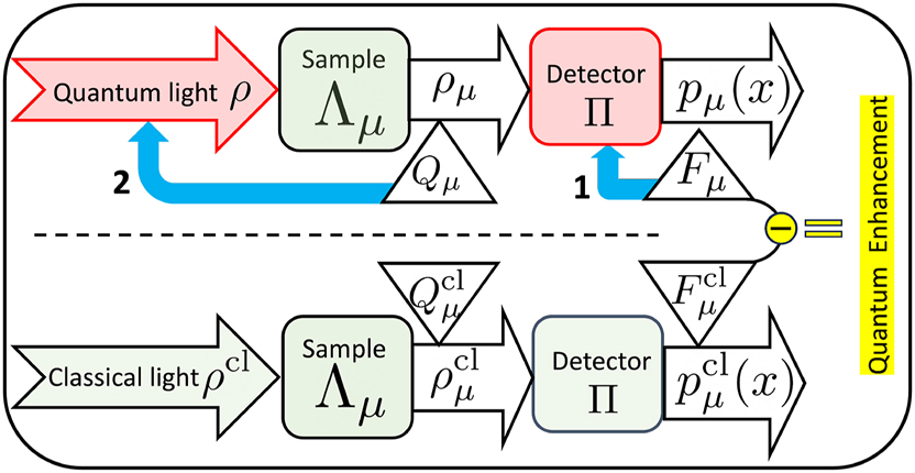
The layout of sensing with quantum light (above dashed line). Corresponding sensing task with classical light (below dashed line). The conceptual route to identifying tangible quantum enhancement lies in the difference of the two classical Fisher informations F
μ
and
I discuss the illusory quadratic quantum scaling that is often the objective of quantum sensing studies in Section 4. I emphasise why it is impossible in the real world and note how tangible quantum advantages may actually be attained. In Section 5, I present some advances in interferometry, microscopy and spectroscopy with quantum light. Rather than an exhaustive record, I select works to identify the main challenges in sensing with quantum light. I end in Section 6 with a collation of these challenges and avenues to directing efforts to overcome them.
2 Sensing
The mathematical formalism describing sensing is a part of information theory and statistics ([13], Chapter 11). It is formally called estimation theory. In the following, I note the classical aspects of the formalism essential for a swift transition to the quantum. While nothing in this formalism is particular to sensing with light and applies in the abstract to any sensor, I will resort to the former for concreteness.
A sensor operates by estimating certain parameters of the light field at its detector. It matters not whether the light came from a distant star or an adjacent nanostructure. The recorded data at the detector {x
1, x
2, …, x
r
} are described mathematically as a statistical model with probability measure p
μ
(x) ≡ p(x|μ), where μ denotes the parameter[1] to be estimated and x labels the output of the detector, such as current, wavelength or photon number. r is the number of recorded data points or repetitions. I choose x and μ to be continuous for now. The performance of a sensor is captured by the accuracy and error of the estimate it provides. If this estimate is denoted by
As the data recorded at the detector are statistical, the performance of a sensor is formally captured by its bias and precision. The former is the expectation value of the accuracy, defined as
Var μ is often called the mean square error. Its square root is the standard deviation.
2.1 Classical estimation theory
To deliver the goal of designing a better sensor, estimation theory is used to identify the smallest possible value of Var μ allowed by laws of probability theory. A central result in classical estimation theory, known as the Cramér–Rao bound states [13]
where
is the classical Fisher information (CFI). For an unbiased estimator,
This inequality is saturated with unbiased estimators under certain regularity conditions on p μ (x). For instance, the maximum likelihood estimator achieves the equality asymptotically [13].
The Cramér–Rao bound shows that variance of an estimator cannot be made arbitrarily small. It thus places a mathematical limit on how precise any sensor can be. This limit is imposed by the amount of information that can extract about a parameter from recorded data. More data or larger r leads to a lower variance. From Eq. (3), it follows that a larger Fisher information and consequently lower variance relies on the recorded data p μ (x) varying strongly with the parameter μ. This is to be expected and is intuitively familiar to all sensor designers.
2.2 Quantum estimation theory
Born rule is the ingredient of quantum mechanics that pertains most directly to sensing. This is unsurprising, as it connects quantum states with observable probabilities. This is the starting point of quantum estimation theory, pioneered in the works of Helstrom [15] and Holevo [16] in quantum information theory.
Mathematically,
where ρ μ denotes the quantum state of the light field, which depends on the parameter μ to be estimated, and Π x is the operator describing the detector outcome x, formally called the positive operator-valued measure (POVM) Π = {Π x } [17]. Inserting Eq. (5) in Eq. (1) shows that the variance Var μ depends on the quantum state ρ μ and the choice of the detector Π. The same holds for the CFI.
This sets the stage for quantum-enhanced sensing, which is a two-step process to improve the precision of a sensor or reduce the corresponding variance by choosing Π and ρ μ judiciously. See Figure 1.
The first step is to minimise the variance Var μ over all physically allowed detectors, that is, POVMs Π. Combining this with Eq. (4) results in the quantum Cramér–Rao bound
where Q μ = max Π F μ is the quantum Fisher information (QFI). The minimisation of the variance translates into a maximisation of the CFI due to reciprocal relation in Eq. (4). This is denoted by the blue arrow numbered 1 in Figure 1. Mathematically [15]
The Hermitian operator L is known as the symmetric logarithmic derivative. The eigenvectors of L are the POVM elements Π x that minimise the variance.
As in classical estimation, the amount of information that can be extracted from a quantum state depends on how strongly it changes with the parameter μ. The operator L is proportional to this rate of change, with the symmetrisation necessary to account for the non-commutative nature of the Hilbert space in which ρ μ resides. The precision of a quantum sensor thus depends solely on the quantum state ρ μ and its derivative with respect to the parameter μ.[2]
Quantum sensors are, at least in principle, no worse than classical sensors. This is because the QFI is greater than or equal to the CFI, that is, Q μ = max Π F μ ≥ F μ . Making this relevant in practice is the fact that there always exists an optimal POVM Π * for which the CFI equals the QFI, that is, the second inequality in Eq. (6) can be saturated. The ease with which Π * may be implemented physically is a technological issue we address later.
The second step is to maximise the QFI Q μ over probe quantum states ρ, where ρ μ = Λ μ [ρ] denoted by the blue arrow numbered 2 in Figure 1. Here, Λ μ [⋅] captures the physics of the sensor that imprints the parameter μ on ρ. For a light-based sensor, this may range from a linear optical element such as a phase shift to an elaborate spectroscopic setup involving nonlinear interactions of a complex quantum system with one or more pulses of light. Mathematically, these can all be described by a completely positive, trace-preserving (CPTP) map [17], which can be obtained from the underlying physical model of the sensor capturing the interaction of the parameter of interest μ with the quantum state ρ of the probe light field. The geometry of the space of CPTP maps plays a central role in determining the performance of quantum sensors in the real world. See Section 4.
A quantum sensor using the probe ρ is, in principle, better than its classical counterpart, if the QFI corresponding to ρ
μ
exceeds that of
But what is ‘classical’ light?
3 Light
‘Classical’ light may, strictly speaking, be considered an oxymoron. This is because light, more formally the electromagnetic field, has a fundamental quantum mechanical description due to Dirac. A very lucid exposition was provided by Fermi [19]. Like many orxymoronic expressions, however, ‘classical’ light has a purchase due to reason, convenience and utility, as I summarise below.
3.1 Classical light
Following the successful development of quantum electrodynamics [20], attention reverted to the quantum mechanical description of optics – quantum optics [21], [22], [23]. It showed that light fields generated by arbitrary distributions of classical currents have an especially simple description in terms of coherent states [21]. The coherent state of the light field of a single mode is thus identified with ‘classical’ light, as is the Poisson distribution of the average occupation number of the nth Fock state |n⟩ – the quantum state with exactly n photons. In this basis, the coherent state is expressed as
where α is a complex number proportional to amplitude of electric field. In my notation, ρ cl = |α⟩⟨α|.
The coherent state ρ cl is, in fact, the quantum mechanical ground state of the Hamiltonian of the free quantum electromagnetic field in absence of charges and currents. This Hamiltonian corresponds to that of an isolated one-dimensional harmonic oscillator [23]. A coherent state is thus a minimum uncertainly wavepacket in the phase space spanned by the position q and momentum p of the oscillator and satisfies
Here,
A coherent state is also very close to the output state of a laser near its threshold [24]. The identification of coherent states as classical light is thus both conceptual and operational, the latter stemming from the ubiquity of high quality of lasers for swathes of the electromagnetic spectrum. I should emphasise that both these routes, via Eq. (11) and the laser, are fundamentally quantum mechanical.
3.2 Quantum light
In the parlance, nonclassical or quantum light is a light field whose state does not have a simple description in terms of coherent states. Technically, a state of light is nonclassical if its Glauber–Sudarshan P-function is not a positive probability density function. Resting on a negative, this definition is quantitively unwieldy. Consequently, a plethora of measures of nonclassicality have developed over time [25], including those relying on other distribution functions [26]. All these measures seek to capture how different a given state of the light field is from a coherent state.
Generating quantum light involves acting on the output of a laser in some way, typically via a nonlinear material. While there is an infinitude of possible quantum states of light, much effort has been directed to generating states with exactly one [27] and two photons [28]. The former often relies on the saturation nonlinearity of a quantum emitter. The emitted single photons can, in principle, be interfered in quantum networks of linear optical elements to produce quantum states of light with a larger number of photons [29].
Quantum states of light can also have an indefinite number of photons. The most prominent in this class are squeezed states [30]. These are, like coherent states, minimum uncertainly wavepackets satisfying Eq. (11), but with the variance in one of the quadratures reduced (or squeezed) at the expense of the other. Their generation relies in the second or third order nonlinear susceptibility of a material. Other quantum states of light can be produced by interfering definite and indefinite photon number states [31]. Yet others, such as superpositions of coherent states called Schrödinger cat states, can be obtained by subtracting photons from squeezed states [32], [33].
3.3 Modes, entanglement and confusion
The quantum states of light I noted above reside in a single mode. A mode is a solution of the electromagnetic wave equation given a set of boundary conditions [34]. They play a central role in the design and operation of nanophotonic devices [35]. Quantum states of light can also be constructed that reside across multiple modes. They could also contain definite or indefinite numbers of photons. An example of the latter is a multimode squeezed state [36].
Quantum entanglement is another notion of nonclassicality. An entangled quantum state of two or more subsystems is defined as one that is not separable, that is, it cannot be expressed a mixture of tensor products of quantum states belonging to the individual subsystems [17]. This is distinct from a state not having a simple description in terms of coherent states, as in Section 3.2. An example is a single-mode squeezed state. It is a nonclassical state but not an entangled state. Quantum light may have entanglement between photons residing in different modes [37].
The indistinguishability of photons in the same mode sometimes confuses matters. This is because the identification of distinct (or distinguishable) subsystems of indistinguishable particles (photons) is not possible. Thus, entanglement between photons in the same mode may be judged unphysical. Indeed, efforts to imbue it with operational information theoretic meaning resorts to the use of modes [38]
4 Quantum sensing – elusive scaling
As the electromagnetic field is defined by an amplitude and a phase, the categories of parameters it can sense are losses, relative phases and their combinations. Amongst these, estimating the difference in the path lengths of light travelling by two different routes from a source to a detector is perhaps the most elementary. This can be cast as relative phase sensing and captures applications ranging from gravitational wave detection [2] to phase-contrast imaging [39]. The formal study of quantum sensing with light has its origins in the work of Helstrom [15] and later in the development of laser-interferometric gravitational wave detectors,[3] which are in effect Michelson interferometers.
Using the formalism from Section 2.2 with μ ≡ ϕ a relative phase parameter,
This quadratic dependence of the QFI of estimating the relative phase on the number of photons is hailed as the hallmark of quantum-enhanced sensing, compared to the QFI for classical light Q ϕ ∼ N where N = |α|2 for ρ cl = |α⟩⟨α|.
The quadratic dependence in Eq. (12) is often dubbed the Heisenberg limit or scaling [42], though its connection to the uncertainly relation in Eq. (11) is tenuous. The quantum states that attain the quadratic scaling in the photon number (exact or average) are certainly nonclassical and include instances such as N00N states and squeezed states [41]. Aspiring for this quadratic scaling in phase estimation has driven much of the interest in quantum-enhanced sensing [43], [44], rooted in seeking a more precise sensor using fewer probe resources. I emphasise that the number of photons actually used is rN. The scaling in r is entirely of classical and statistical origin and not subject to quadratic quantum enhancements.
A central challenge is the production of quantum states of light with large photon numbers at a repetition rate comparable to a coherent state, which can easily have billions or trillions of photons. ‘Bright’ squeezed states with comparable mean photon numbers have been reported recently [45]. Preparing quantum states with high fixed photon number remains hard despite novel theoretical ideas [46], [47]. Should such ideas become realisable, their integration in to the wider quantum photonic sensing architecture would be most welcome.
The quadratic scaling for phase estimation is impossible in real-world sensing scenarios even if desirable quantum states are available. This is because all real world sensors inevitably encounter losses and other noise or decoherence processes [48]. Consequently, the best possible scaling is
where c is a constant independent of N. It depends on the nature and strength of the loss, noise or decoherence processes.
The quadratic scaling for phase estimation in Eq. (12) in the absence of loss and noise also applies to any parameter μ generated by a Λ μ that is a unitary map. The concomitant linear scaling in Eq. (13) then applies to it in the real world. The QFI associated with the estimation of parameters, such as (linear) loss or absorption, have such a linear dependence on N to start with.
The root of the linear scaling in Eq. (13) lies in the geometry of the space of CPTP maps Λ
μ
[48]. This space is convex, that is, if
Maps that cannot be decomposed into a convex combination of other maps are called extremal. An instance of an extremal map is a unitary such as U ϕ , which lead to the quadratic scaling in Eq. (12). The linear scaling in Eq. (13) is thus, if possibly abstract, of most fundamental origins and seemingly insurmountable. Consequently, all stakeholders in the field of quantum sensing must recognise it.
The constant c has been evaluated analytically for widely prevalent processes such as photon loss, dephasing and spontaneous emission [48]. These suggest that diminishing losses and decoherence increase the value of c. While its exact behaviour depends on the details of the sensor as well as the loss and noise processes, the magnitude of c can be increased with improved technology, leading to possibly substantial tangible quantum enhancements in sensing.
5 Sensing modalities
In my view, the future of quantum-enhanced sensing rests on increasing the constant c. This depends on the specifics of the sensing modality. From the domain of umpteen sensing modalities [49], [50], even with light [4], [5], [6], [8], [9], [10], I will focus on three in this section. If this suggests that the drive for quantum-enhanced sensing to be platform and application specific, it is only partially true. In the following, I will highlight some general concepts and insights that are applicable across sensing domains and modalities while restricting myself to three common paradigms with relevance for nanophotonics.
5.1 Interferometry
I begin with the estimation of a relative phase, the natural sensing task emanating from interferometry. A real linear interferometer, especially implemented using integrated photonics, is subject to losses [51], [52]. These are typically assumed to be linear and associated with the preparation η p and detection η d , as well as the sensing of the phase ϕ itself η. The performance of the quantum sensor in Figure 2, with fixed-photon-number state inputs and photon-number-resolving detectors (PNRDs), is quantified by the CFI of estimating ϕ using the formalism of Section 2.2. For quantum enhancement, this must exceed the CFI of estimating ϕ using classical light with |α|2 = 2N, as noted in Figure 1. This is only possible if the losses are such as to lie within a region of the unit cube of η p , η, η d as shown for N = 1 and N = 3 in Figure 3. I extract two observations from them.
![Figure 2:
Relative phase ϕ estimation in a linear interferometer, where η
p
, η and η
d
are the preparation, transmission and detection losses, respectively. η
p
= η = η
d
= 1 denotes no losses. Taken from Ref. [51].](/document/doi/10.1515/nanoph-2024-0649/asset/graphic/j_nanoph-2024-0649_fig_002.jpg)
Relative phase ϕ estimation in a linear interferometer, where η p , η and η d are the preparation, transmission and detection losses, respectively. η p = η = η d = 1 denotes no losses. Taken from Ref. [51].
![Figure 3:
Region of (η
p
, η, η
d
) space of losses for which quantum enhancement is possible using N = 1 (left) and N = 3 (right) in the sensor in Figure 2. Taken from Ref. [51].](/document/doi/10.1515/nanoph-2024-0649/asset/graphic/j_nanoph-2024-0649_fig_003.jpg)
The first observation is that the most demanding call is placed on the detector efficiency η d . In other words, high-efficiency PNRDs are necessary for phase estimation with quantum light using a linear interferometer as envisaged in Figure 2, to outperform its classical counterpart. This is because the most damage to a quantum state in sensor occurs when the quantum light has picked up all the information it can about the parameter to be estimated.
Integrated, high-efficiency PNRDs have become available in recent years [53]. To minimise losses in the preparation, the source of the quantum light can be placed on the same integrated chip. This is also becoming possible [54]. Finally, placing the sample on the same platform is essential to fulfil the vision of quantum nanophotonic sensing, especially in biomedical settings. This remains a challenge even in nanophotonic biosensing with classical light ([55], Fig. 4) as is that of having sources and detectors operating at light wavelengths most relevant for the sample [56].
The second observation is that the demand on η d is greater for the larger N. The same applies to η p . While having more photons does allow greater protection from transmission losses η, the performance of the sensor is limited by its most demanding component η d . Quantum states with more photons are by themselves thus not enough for a better quantum sensor. Indeed, classical states of light are more robust against losses than quantum states. Better quantum sensors thus need detectors with efficiency increasing with N, and number resolvability. These do not make for a scalable approach for quantum enhanced sensing.
Quantum error correction might counter losses in a scalable manner. Some theoretical works have shown that quantum error correction can indeed combat certain kinds of noise processes in sensing [57], [58], [59], [60]. These and other works [61] find that the elusive quadratic scaling of Eq. (12) can be recovered but require unphysical error correcting operations such as infinitely fast ones. They also rely on unphysical assumptions such as perfect error correcting operations. Experimentally, quantum error correction does help improve quantum sensing for small N by combating certain kinds of noise in nitrogen-vacancy centre based magnetometry [62]. Similar demonstrations against loss in sensing with quantum light would be exciting.
All real-world error-correction operations are themselves error prone. Combating that requires fault tolerance. Fault-tolerant quantum sensing has been explored theoretically [63]. It identified two categories of noise: (i) beyond our control, associated with sensing the parameter, and (ii) under our control, associated with in operations such as preparing, manipulating and measuring probes and ancillae. It then introduced noise thresholds to quantify the noise resilience of parameter estimation schemes, and theoretically demonstrated improved noise thresholds over the non-fault-tolerant schemes. More importantly, it showed that better devices, which can be engineered under our control, can counter larger noise beyond our control. The use of bespoke quantum error correcting codes for combating losses would identify the efficacy of fault-tolerant sensing with quantum light.
Despite the specificity of the sensing modality in this subsection, I hope that both the importance of detectors and centrality of combating losses in a scalable manner are general aspects of sensing with quantum light worth recognising. Quantum sensor designers may feel the suggested remedy of deploying the machinery of quantum fault tolerance excessive and foreign. This feeling is perhaps nurtured by the belief that building a quantum sensor ought to be an easier endeavour than building a quantum computer, the domain to which fault tolerance is typically associated. As quantum light with more photons become available and losses which are determined by material properties of sensors and detectors cannot be reduced in proportion, experimenters may be forced to tread the path traced above.
5.2 Microscopy
I now move to microscopy with quantum light. The set of possibilities is immense even within optical microscopy.[4] Following the strategy noted in Figure 1, I focus on microscopy with quantum light that improves upon classical schemes limited by shot noise [66], [67]. Shot noise is attributed to the Poissionian photon number distribution of the coherent state and identified with the linear scaling of the QFI for coherent states noted in Section 4. Brighter coherent state pulses can give more precision but lead to greater photodamage of the sample, a particular concern in biomedical applications. The strength of the coherent state thus limited, the purpose of microscopy with quantum light is to continue improving the precision.
Quantum enhanced stimulated emission microscopy [68] and quantum enhanced stimulated Raman spectroscopy [69], [70] achieve this goal. The latter work also undertook a detailed study of photodamage. These detect the concentration of a sample, which is proportional to the number of photons absorbed (or lost) from a probe pulse. Mathematically, the best quantum state for estimating loss is a Fock state with a fixed number of photons, say |n⟩ [71]. This because on the quantum state after the loss is
Another abiding principle, essential for sensing with quantum light to be worthwhile, is to operate in a shot-noise-limited regime. In other words, the classical method must be limited in a manner that quantum ones can improve upon. This is typically not the case. Indeed, operating a shot-noise-limited classical sensor may be harder in practice than imposing quantum enhancements on it. In many optical sensors as in the microscopy schemes noted above, the classical noise sources such as technical laser noise and photodetector electronic noise dominate the shot noise at low frequencies. This is overcome by modulating the signal at a few megaHertz where shot noise is dominant. Intensity-squeezed coherent states of light then perform quantum-enhanced microscopy.
Generating intensity-squeezed coherent states of light is easier than high-n Fock states but harder than coherent states. The challenge arises due to incomplete understanding of nonlinear process of a pulsed nature such as group velocity mismatch between the pump and seed pulses, beam divergence, spatial walk-off or spatiotemporal coupling in the parametric gain [68]. Furthermore, higher gain, which is necessary for more squeezing and hence quantum enhancement, requires a more thorough analysis [72] than low gain efforts providing a squeezing of a dB or lower. This ties back to the challenge of producing quantum states of light with large photon numbers and high repetition rates, as noted in Section 4.
This modality once again highlights the challenge of generating quantum states of light with large numbers of photons. Another crucial issue in sensing with quantum light is identifying the limitation of the corresponding sensor using classical light. It must be that the classical nature of the light – shot noise is the limitation in the classical sensor. Attaining that limit, which may be a nontrivial experimental and technological step in itself, is essential before embarking on sensing with quantum light.
5.3 Spectroscopy
I finally turn to spectroscopy, perhaps the most ubiquitous of analytical tools in the natural sciences. I also expand to a paradigm where Λ μ captures the interaction between quantum light and quantum matter from the first principles of quantum mechanics. Effective quantities such as phase and loss discussed the last two sensing modalities are functions of the underlying ‘microscopic’ parameters of the quantum matter system such as transition energies, line widths or lifetimes, dipole–dipole couplings, electron–phonon couplings, etc. This expanded paradigm leads to an operational definition of spectroscopy as the precise estimation of these ‘microscopic’ parameters. It is also more informative when novel complex quantum matter systems are studied spectroscopically than merely estimating effective macroscopic parameters such as absorption and refractive index.
Contemporary theoretical studies of spectroscopy treat the light classically, leading to a semiclassical light–matter interaction [73]. Formally, the total Hamiltonian
captures the operation Λ
μ
[ρ
cl], where
Early experiments efforts towards quantum light spectroscopy used classical laser light to measure semiconductor quantum wells and processed the data to mimic the response of the system to a quantum state of light [74]. Early theoretical works did study the effect of shining quantum light directly on complex quantum systems. They evaluated the signal for specific spectroscopic configurations and measurement schemes [75] and showed that some excitation transfer pathways in coupled quantum systems obscured in nonlinear spectroscopy using classical light could be revealed by using quantum light. As these studies work with specific input states and measurements, they are incapable of optimising over input states and measurements as outlined in Section 2.2 and Figure 1.
Recent works have cast spectroscopy in the framework of quantum estimation theory to begin traversing the path outlined in Figure 1. It relies on calculating the quantum state of the light pulse Λ μ [ρ] after it has interacted with a quantum matter system, as in Figure 4. This is the central ingredient in the evaluation of the QFI of estimating ‘microscopic’ parameters of the matter system and identification of optimal measurements [76], [77]. These works reproduce known results on absorption spectroscopy when a two-level system (TLS) starts in the ground state and should do so for stimulated emission spectroscopy when the TLS starts in an excited state.
![Figure 4:
Illustration (not to scale) of the excitation of quantum matter system by a quantum pulse of light (with Gaussian temporal envelope). Γ represents the interaction strength with the pulse, while Γ⊥ describes emission into other (inaccessible) orthogonal field modes. As illustrated, the shape of the wave packet is changed by the interaction with the matter system. Taken from Ref. [76]](/document/doi/10.1515/nanoph-2024-0649/asset/graphic/j_nanoph-2024-0649_fig_004.jpg)
Illustration (not to scale) of the excitation of quantum matter system by a quantum pulse of light (with Gaussian temporal envelope). Γ represents the interaction strength with the pulse, while Γ⊥ describes emission into other (inaccessible) orthogonal field modes. As illustrated, the shape of the wave packet is changed by the interaction with the matter system. Taken from Ref. [76]
The new insight from this formalism is that additional information about the matter system is available in the distorted quantum light pulse after the interaction. This is in addition to the information that can be extracted from absorption or emission spectroscopy. In other words, beyond counting the number of photons, there is more information in the shape of the pulse itself that can be extracted from quantum light spectroscopy, as illustrated in Figure 4. The relative contributions depend on the time duration of the experiment relative to the lifetime, as well as the fraction Γ/Γ⊥ of the light detected.
Another novel insight is that higher precision in estimating a parameter such as lifetime is not coincident with higher excitation probability or cross section [76]. This is significant as the latter is often taken to be a surrogate for the efficacy of spectroscopy [78]. Other insights can be extracted using entangled quantum states as probes such as biphotons and more involved matter systems such as coupled dimers [79].
Extracting this additional information from the pulse shape requires temporal or spectral mode-resolved measurements. Such measurements are now available [80] for single photons. Non-destructive photon number counting is necessary to extract the information from absorption or emission spectroscopy simultaneously. This is more challenging for single photons at optical wavelengths. The strength of the formalism also lies in showing what is unnecessary. For instance, entangled measurements are not necessary to attain the best fundamental precision if only one mode of a biphoton state interacts with the sample, as in Figure 5.
![Figure 5:
Schematic of pulsed biphoton spectroscopy. Taken from Ref. [79]](/document/doi/10.1515/nanoph-2024-0649/asset/graphic/j_nanoph-2024-0649_fig_005.jpg)
Schematic of pulsed biphoton spectroscopy. Taken from Ref. [79]
To obtain the quantum state Λ
μ
[ρ] of the pulse of light after the interaction, the dynamical equations of quantum mechanics such as the Schrödinger equation for the Hamiltonian in Eq. (14) must be solved. For pulsed interactions,
Quantum light spectroscopy is deeply intertwined the study of quantum light–matter interactions, especially in quantum nanophotonics. The latter engineers configurations that can enhance the light–matter interaction to probe the physics of quantum matter systems such as complex molecules. Cavities, waveguides and surfaces provide the varied platforms to perform quantum light spectroscopy, including providing sources of quantum light. Combining these with integrated photonic setups with efficient detectors ([84], Fig. 10) could vastly expand the arena of quantum light spectroscopy into domains such as quantum nanophotonic biosensing [55].
6 Conclusions
I conclude with an enumerated gist of the vital challenges in sensing with quantum light and possible avenues for overcoming them.
Detecting quantum states of light with high efficiency. This is to make the most of the available quantum states of light. The efforts will have to be in material science and technology.
Generating ‘bright’ quantum states of light with large numbers of photons at repetition rates and determinacy comparable to classical sources. The efforts should be in developing sources of ‘bright’ squeezed states of light.
Combat inevitable losses in the sensing process by develop error correction and fault tolerance for quantum sensing. The efforts will have to be in quantum information and coding theory.
Integrating sources, interactions and detectors on the same platform. This will be pulled by specific applications and pushed by fabrication technologies.
Funding source: European Union’s Horizon Europe
Award Identifier / Grant number: 101070700 (MIRAQLS).
Acknowledgments
I thank my numerous colleagues and collaborators for stimulating discussions over the years.
-
Research funding: This work was supported, in part, by grant from the UKRI (Reference Number: 10038209) under the UK Government’s Horizon Europe Guarantee for the European Union’s Horizon Europe Research and Innovation Programme under agreement 101070700 (MIRAQLS).
-
Author contributions: The author confirms the sole responsibility for the conception of the study, presented results and manuscript preparation.
-
Conflict of interest: Author states no conflicts of interest.
-
Data availability: Data sharing is not applicable to this article as no datasets were generated or analysed during the current study.
References
[1] I. A. Walmsley, “Quantum optics: Science and technology in a new light,” Science, vol. 348, no. 6234, pp. 525–530, 2015. https://doi.org/10.1126/science.aab0097.Search in Google Scholar PubMed
[2] C. M. Caves, “Quantum-mechanical noise in an interferometer,” Phys. Rev. D, vol. 23, no. 8, p. 1693, 1981. https://doi.org/10.1103/physrevd.23.1693.Search in Google Scholar
[3] R. Schnabel, N. Mavalvala, D. E. McClelland, and P. K. Lam, “Quantum metrology for gravitational wave astronomy,” Nat. Commun., vol. 1, no. 1, p. 121, 2010. https://doi.org/10.1038/ncomms1122.Search in Google Scholar PubMed
[4] M. A. Taylor and W. P. Bowen, “Quantum metrology and its application in biology,” Phys. Rep., vol. 615, pp. 1–59, 2016, https://doi.org/10.1016/j.physrep.2015.12.002.Search in Google Scholar
[5] B. J. Lawrie, P. D. Lett, A. M. Marino, and R. C. Pooser, “Quantum sensing with squeezed light,” ACS Photonics, vol. 6, no. 6, pp. 1307–1318, 2019. https://doi.org/10.1021/acsphotonics.9b00250.Search in Google Scholar
[6] I. R. Berchera and I. P. Degiovanni, “Quantum imaging with sub-poissonian light: Challenges and perspectives in optical metrology,” Metrologia, vol. 56, no. 2, p. 024001, 2019. https://doi.org/10.1088/1681-7575/aaf7b2.Search in Google Scholar
[7] S. Szoke, H. Liu, B. P. Hickam, M. He, and S. K. Cushing, “Entangled light–matter interactions and spectroscopy,” J. Mater. Chem. C, vol. 8, no. 31, pp. 10732–10741, 2020. https://doi.org/10.1039/d0tc02300k.Search in Google Scholar
[8] C. Lee, B. Lawrie, R. Pooser, K.-G. Lee, C. Rockstuhl, and M. Tame, “Quantum plasmonic sensors,” Chem. Rev., vol. 121, no. 8, p. 4743, 2021. https://doi.org/10.1021/acs.chemrev.0c01028.Search in Google Scholar PubMed
[9] L. Kim, H. Choi, M. E. Trusheim, H. Wang, and D. R. Englund, “Nanophotonic quantum sensing with engineered spin-optic coupling,” Nanophotonics, vol. 12, no. 3, pp. 441–449, 2023. https://doi.org/10.1515/nanoph-2022-0682.Search in Google Scholar PubMed PubMed Central
[10] H. Defienne, et al.., “Advances in quantum imaging,” Nat. Photonics, vol. 18, no. 10, p. 1024, 2024. https://doi.org/10.1038/s41566-024-01516-w.Search in Google Scholar
[11] E. Moreva, et al.., “Quantum photonics sensing in biosystems,” APL Photonics, vol. 10, no. 1, p. 010902, 2025. https://doi.org/10.1063/5.0232183.Search in Google Scholar
[12] D. Ganapathy, et al.., LIGO O4 Detector Collaboration, “Broadband quantum enhancement of the LIGO detectors with frequency-dependent squeezing,” Phys. Rev. X, vol. 13, p. 041021, 2023. https://doi.org/10.1103/PhysRevX.13.041021.Search in Google Scholar
[13] T. M. Cover and J. A. Thomas, Elements of Information Theory, 2nd ed. Nashville, TN, John Wiley & Sons, 2006.Search in Google Scholar
[14] F. Albarelli, M. Barbieri, M. G. Genoni, and I. Gianani, “A perspective on multiparameter quantum metrology: From theoretical tools to applications in quantum imaging,” Phys. Lett. A, vol. 384, no. 12, p. 126311, 2020. https://doi.org/10.1016/j.physleta.2020.126311.Search in Google Scholar
[15] C. W. Helstrom, “Quantum detection and estimation theory,” in Mathematics in Science and Engineering, San Diego, CA, Academic Press, 1976.Search in Google Scholar
[16] A. S. Holevo, Probabilistic and Statistical Aspects of Quantum Theory, Monographs (Scuola Normale Superiore), 1st ed. Pisa, Switzerland, Edizioni della Normale, 2011.Search in Google Scholar
[17] M. A. Nielsen and I. L. Chuang, Quantum Computation and Quantum Information, Cambridge, England, Cambridge University Press, 2010.Search in Google Scholar
[18] S. Personick, “Application of quantum estimation theory to analog communication over quantum channels,” IEEE Trans. Inf. Theor., vol. 17, no. 3, pp. 240–246, 1971. https://doi.org/10.1109/tit.1971.1054643.Search in Google Scholar
[19] E. Fermi, “Quantum theory of radiation,” Rev. Mod. Phys., vol. 4, no. 1, p. 87, 1932. https://doi.org/10.1103/revmodphys.4.87.Search in Google Scholar
[20] S. S. Schweber, “Qed and the men who made it,” in Princeton Series in Physics, Princeton, NJ, Princeton University Press, 1994.Search in Google Scholar
[21] R. J. Glauber, “Photon correlations,” Phys. Rev. Lett., vol. 10, no. 3, p. 84, 1963. https://doi.org/10.1103/physrevlett.10.84.Search in Google Scholar
[22] E. C. G. Sudarshan, “Equivalence of semiclassical and quantum mechanical descriptions of statistical light beams,” Phys. Rev. Lett., vol. 10, no. 7, p. 277, 1963. https://doi.org/10.1103/physrevlett.10.277.Search in Google Scholar
[23] R. J. Glauber, “Coherent and incoherent states of the radiation field,” Phys. Rev., vol. 131, no. 6, p. 2766, 1963. https://doi.org/10.1103/physrev.131.2766.Search in Google Scholar
[24] J. Gea-Banacloche, “Emergence of classical radiation fields through decoherence in the scully-lamb laser model,” Found. Phys., vol. 28, no. 4, pp. 531–548, 1998. https://doi.org/10.1023/a:1018729904161.10.1023/A:1018729904161Search in Google Scholar
[25] K. C. Tan and H. Jeong, “Nonclassical light and metrological power: An introductory review,” AVS Quant. Sci., vol. 1, no. 1, p. 014701, 2019. https://doi.org/10.1116/1.5126696.Search in Google Scholar
[26] M. Hillery, R. O’Connell, M. Scully, and E. Wigner, “Distribution functions in physics: Fundamentals,” Phys. Rep., vol. 106, no. 3, pp. 121–167, 1984. https://doi.org/10.1016/0370-1573(84)90160-1.Search in Google Scholar
[27] E. Meyer-Scott, C. Silberhorn, and A. Migdall, “Single-photon sources: Approaching the ideal through multiplexing,” Rev. Sci. Instrum., vol. 91, no. 4, p. 041101, 2020. https://doi.org/10.1063/5.0003320.Search in Google Scholar PubMed PubMed Central
[28] A. S. Solntsev and A. A. Sukhorukov, “Path-entangled photon sources on nonlinear chips,” Rev. Phys., vol. 2, pp. 19–31, 2017, https://doi.org/10.1016/j.revip.2016.11.003.Search in Google Scholar
[29] W. R. Clements, P. C. Humphreys, B. J. Metcalf, W. S. Kolthammer, and I. A. Walmsley, “Optimal design for universal multiport interferometers,” Optica, vol. 3, no. 12, p. 1460, 2016. https://doi.org/10.1364/optica.3.001460.Search in Google Scholar
[30] R. Schnabel, “Squeezed states of light and their applications in laser interferometers,” Phys. Rep., vol. 684, p. 1, 2017, https://doi.org/10.1016/j.physrep.2017.04.001.Search in Google Scholar
[31] T. J. Bartley, et al.., “Multiphoton state engineering by heralded interference between single photons and Coherent states,” Phys. Rev. A, vol. 86, no. 4, p. 043820, 2012. https://doi.org/10.1103/physreva.86.043820.Search in Google Scholar
[32] K. Wakui, H. Takahashi, A. Furusawa, and M. Sasaki, “Photon subtracted squeezed states generated with periodically poled KTiOPO4,” Opt. Express, vol. 15, no. 6, p. 3568, 2007. https://doi.org/10.1364/oe.15.003568.Search in Google Scholar PubMed
[33] T. J. Bartley, P. J. D. Crowley, A. Datta, J. Nunn, L. Zhang, and I. Walmsley, “Strategies for enhancing quantum entanglement by local photon subtraction,” Phys. Rev. A, vol. 87, no. 2, p. 022313, 2013. https://doi.org/10.1103/physreva.87.022313.Search in Google Scholar
[34] R. Dändliker, Education and Training in Optics and Photonics, Washington, DC, Optica Publishing Group, 1999, p. GP193.Search in Google Scholar
[35] J. Lu and J. Vučković, “Nanophotonic computational design,” Opt. Express, vol. 21, no. 11, p. 13351, 2013. https://doi.org/10.1364/oe.21.013351.Search in Google Scholar PubMed
[36] Y. Cai, et al.., “Multimode entanglement in reconfigurable graph states using optical frequency combs,” Nat. Commun., vol. 8, no. 1, p. 15645, 2017. https://doi.org/10.1038/ncomms15645.Search in Google Scholar PubMed PubMed Central
[37] S. Walborn, C. Monken, S. Pádua, and P. Souto Ribeiro, “Spatial correlations in parametric down-conversion,” Phys. Rep., vol. 495, no. 4–5, p. 87, 2010. https://doi.org/10.1016/j.physrep.2010.06.003.Search in Google Scholar
[38] F. Benatti, R. Floreanini, F. Franchini, and U. Marzolino, “Entanglement in indistinguishable particle systems,” Phys. Rep., vol. 878, p. 1, 2020, entanglement in indistinguishable particle systems, https://doi.org/10.1016/j.physrep.2020.07.003.Search in Google Scholar
[39] P. C. Humphreys, M. Barbieri, A. Datta, and I. A. Walmsley, “Quantum enhanced multiple phase estimation,” Phys. Rev. Lett., vol. 111, no. 7, p. 070403, 2013. https://doi.org/10.1103/physrevlett.111.070403.Search in Google Scholar
[40] S. L. Braunstein, C. M. Caves, and G. Milburn, “Generalized uncertainty relations: Theory, examples, and lorentz invariance,” Ann. Phys., vol. 247, no. 1, pp. 135–173, 1996. https://doi.org/10.1006/aphy.1996.0040.Search in Google Scholar
[41] M. D. Lang and C. M. Caves, “Optimal quantum-enhanced interferometry,” Phys. Rev. A, vol. 90, no. 2, p. 025802, 2014. https://doi.org/10.1103/physreva.90.025802.Search in Google Scholar
[42] M. J. Holland and K. Burnett, “Interferometric detection of optical phase shifts at the Heisenberg limit,” Phys. Rev. Lett., vol. 71, no. 9, p. 1355, 1993. https://doi.org/10.1103/physrevlett.71.1355.Search in Google Scholar PubMed
[43] V. Giovannetti, S. Lloyd, and L. Maccone, “Quantum-enhanced measurements: Beating the standard quantum limit,” Science, vol. 306, no. 5700, pp. 1330–1336, 2004. https://doi.org/10.1126/science.1104149.Search in Google Scholar PubMed
[44] V. Giovannetti, S. Lloyd, and L. Maccone, “Advances in quantum metrology,” Nat. Photonics, vol. 5, no. 4, pp. 222–229, 2011. https://doi.org/10.1038/nphoton.2011.35.Search in Google Scholar
[45] A. Rasputnyi, et al.., “High-harmonic generation by a bright squeezed vacuum,” Nat. Phys., vol. 20, no. 12, pp. 1960–1965, 2024. https://doi.org/10.1038/s41567-024-02659-x.Search in Google Scholar
[46] N. Rivera, J. Sloan, Y. Salamin, J. D. Joannopoulos, and M. Soljačić, “Creating large fock states and massively squeezed states in optics using systems with nonlinear bound states in the continuum,” Proc. Natl. Acad. Sci. U. S. A., vol. 120, no. 9, 2023, Art no. e2219208120. https://doi.org/10.1073/pnas.2219208120.Search in Google Scholar PubMed PubMed Central
[47] A. M. de las Heras, D. Porras, and A. González-Tudela, arXiv:2411.07929, 2024.Search in Google Scholar
[48] R. Demkowicz-Dobrzański, J. Kołodyński, and M. Guţă, “The elusive Heisenberg limit in quantum-enhanced metrology,” Nat. Commun., vol. 3, no. 1, p. 1063, 2012. https://doi.org/10.1038/ncomms2067.Search in Google Scholar PubMed PubMed Central
[49] C. L. Degen, F. Reinhard, and P. Cappellaro, “Quantum sensing,” Rev. Mod. Phys., vol. 89, no. 3, p. 035002, 2017. https://doi.org/10.1103/revmodphys.89.035002.Search in Google Scholar
[50] C.-J. Yu, S. von Kugelgen, D. W. Laorenza, and D. E. Freedman, “A molecular approach to quantum sensing,” ACS Cent. Sci., vol. 7, no. 5, p. 712, 2021. https://doi.org/10.1021/acscentsci.0c00737.Search in Google Scholar PubMed PubMed Central
[51] A. Datta, L. Zhang, N. Thomas-Peter, U. Dorner, B. J. Smith, and I. A. Walmsley, “Quantum metrology with imperfect states and detectors,” Phys. Rev. A, vol. 83, no. 6, p. 063836, 2011. https://doi.org/10.1103/physreva.83.063836.Search in Google Scholar
[52] N. Thomas-Peter, et al.., “Integrated photonic sensing,” New J. Phys., vol. 13, no. 5, p. 055024, 2011. https://doi.org/10.1088/1367-2630/13/5/055024.Search in Google Scholar
[53] J. P. Höpker, et al.., “Integrated transition edge sensors on titanium in-diffused lithium niobate waveguides,” APL Photonics, vol. 4, no. 5, p. 056103, 2019. https://doi.org/10.1063/1.5086276.Search in Google Scholar
[54] H. S. Stokowski, et al.., “Integrated quantum optical phase sensor in thin film lithium niobate,” Nat. Commun., vol. 14, no. 1, p. 3355, 2023. https://doi.org/10.1038/s41467-023-38246-6.Search in Google Scholar PubMed PubMed Central
[55] H. Altug, S.-H. Oh, S. A. Maier, and J. Homola, “Advances and applications of nanophotonic biosensors,” Nat. Nanotechnol., vol. 17, no. 1, pp. 5–16, 2022. https://doi.org/10.1038/s41565-021-01045-5.Search in Google Scholar PubMed
[56] Y. Todorov, S. Dhillon, and J. Mangeney, “Thz quantum gap: Exploring potential approaches for generating and detecting non-classical states of Thz light,” Nanophotonics, vol. 13, no. 10, pp. 1681–1691, 2024. https://doi.org/10.1515/nanoph-2023-0757.Search in Google Scholar PubMed PubMed Central
[57] J. Preskill, arXiv:quant-ph/0010098, 2000.10.1002/ev.1189Search in Google Scholar
[58] W. Dür, M. Skotiniotis, F. Fröwis, and B. Kraus, “Improved quantum metrology using quantum error correction,” Phys. Rev. Lett., vol. 112, no. 8, p. 080801, 2014. https://doi.org/10.1103/physrevlett.112.080801.Search in Google Scholar
[59] G. Arrad, Y. Vinkler, D. Aharonov, and A. Retzker, “Increasing sensing resolution with error correction,” Phys. Rev. Lett., vol. 112, no. 15, p. 150801, 2014. https://doi.org/10.1103/physrevlett.112.150801.Search in Google Scholar
[60] D. A. Herrera-Martí, T. Gefen, D. Aharonov, N. Katz, and A. Retzker, “Quantum error-correction-enhanced magnetometer overcoming the limit imposed by relaxation,” Phys. Rev. Lett., vol. 115, no. 20, p. 200501, 2015. https://doi.org/10.1103/physrevlett.115.200501.Search in Google Scholar PubMed
[61] S. Zhou, M. Zhang, J. Preskill, and L. Jiang, “Achieving the Heisenberg limit in quantum metrology using quantum error correction,” Nat. Commun., vol. 9, no. 1, p. 78, 2018. https://doi.org/10.1038/s41467-017-02510-3.Search in Google Scholar PubMed PubMed Central
[62] T. Unden, et al.., “Quantum metrology enhanced by repetitive quantum error correction,” Phys. Rev. Lett., vol. 116, no. 23, p. 230502, 2016. https://doi.org/10.1103/physrevlett.116.230502.Search in Google Scholar PubMed
[63] T. Kapourniotis and A. Datta, “Fault-tolerant quantum metrology,” Phys. Rev. A, vol. 100, no. 2, p. 022335, 2019. https://doi.org/10.1103/physreva.100.022335.Search in Google Scholar
[64] M. Tsang, R. Nair, and X.-M. Lu, “Quantum theory of super resolution for two incoherent optical point sources,” Phys. Rev. X, vol. 6, no. 3, p. 031033, 2016. https://doi.org/10.1103/physrevx.6.031033.Search in Google Scholar
[65] M. Tsang, “Subdiffraction incoherent optical imaging via spatial-mode demultiplexing,” New J. Phys., vol. 19, no. 2, p. 023054, 2017. https://doi.org/10.1088/1367-2630/aa60ee.Search in Google Scholar
[66] W. Min, S. Lu, S. Chong, R. Roy, G. R. Holtom, and X. S. Xie, “Imaging chromophores with undetectable fluorescence by stimulated emission microscopy,” Nature, vol. 461, no. 7267, pp. 1105–1109, 2009. https://doi.org/10.1038/nature08438.Search in Google Scholar PubMed
[67] C. W. Freudiger, W. Yang, G. R. Holtom, N. Peyghambarian, X. S. Xie, and K. Q. Kieu, “Stimulated Raman scattering microscopy with a Robust fibre laser source,” Nat. Photonics, vol. 8, no. 2, pp. 153–159, 2014. https://doi.org/10.1038/nphoton.2013.360.Search in Google Scholar PubMed PubMed Central
[68] G. Triginer Garces, et al.., “Quantum-enhanced stimulated emission detection for label-free microscopy,” Appl. Phys. Lett., vol. 117, no. 2, p. 024002, 2020. https://doi.org/10.1063/5.0009681.Search in Google Scholar
[69] R. B. de Andrade, H. Kerdoncuff, K. Berg-Sørensen, T. Gehring, M. Lassen, and U. L. Andersen, “Quantum-enhanced continuous-wave stimulated Raman scattering spectroscopy,” Optica, vol. 7, no. 5, p. 470, 2020. https://doi.org/10.1364/optica.386584.Search in Google Scholar
[70] C. A. Casacio, et al.., “Quantum-enhanced nonlinear microscopy,” Nature, vol. 594, no. 7862, p. 201, 2021. https://doi.org/10.1038/s41586-021-03528-w.Search in Google Scholar PubMed
[71] G. Adesso, F. Dell’Anno, S. De Siena, F. Illuminati, and L. A. M. Souza, “Optimal estimation of losses at the ultimate quantum limit with non-gaussian states,” Phys. Rev. A, vol. 79, no. 4, p. 040305, 2009. https://doi.org/10.1103/physreva.79.040305.Search in Google Scholar
[72] N. Quesada, G. Triginer, M. D. Vidrighin, and J. E. Sipe, “Theory of high-gain twin-beam generation in waveguides: From Maxwell’s equations to efficient simulation,” Phys. Rev. A, vol. 102, no. 3, p. 033519, 2020. https://doi.org/10.1103/physreva.102.033519.Search in Google Scholar
[73] S. Mukamel, Principles of Nonlinear Optical Spectroscopy, Oxford Series in Optical & Imaging Sciences, New York, NY, Oxford University Press, 1999.Search in Google Scholar
[74] M. Kira, S. W. Koch, R. P. Smith, A. E. Hunter, and S. T. Cundiff, “Quantum spectroscopy with Schrödinger-Cat states,” Nat. Phys., vol. 7, no. 10, pp. 799–804, 2011. https://doi.org/10.1038/nphys2091.Search in Google Scholar
[75] K. E. Dorfman, F. Schlawin, and S. Mukamel, “Nonlinear optical signals and spectroscopy with quantum light,” Rev. Mod. Phys., vol. 88, no. 4, p. 045008, 2016. https://doi.org/10.1103/revmodphys.88.045008.Search in Google Scholar
[76] F. Albarelli, E. Bisketzi, A. Khan, and A. Datta, “Fundamental limits of pulsed quantum light spectroscopy: Dipole moment estimation,” Phys. Rev. A, vol. 107, no. 6, p. 062601, 2023. https://doi.org/10.1103/physreva.107.062601.Search in Google Scholar
[77] E. Darsheshdar, A. Khan, F. Albarelli, and A. Datta, “Role of chirping in pulsed single-photon spectroscopy,” Phys. Rev. A, vol. 110, no. 4, p. 043710, 2024. https://doi.org/10.1103/physreva.110.043710.Search in Google Scholar
[78] M. G. Raymer, T. Landes, and A. H. Marcus, “Entangled two-photon absorption by atoms and molecules: A quantum optics tutorial,” J. Chem. Phys., vol. 155, no. 8, p. 081501, 2021. https://doi.org/10.1063/5.0049338.Search in Google Scholar PubMed
[79] A. Khan, F. Albarelli, and A. Datta, “Does entanglement enhance single-molecule pulsed biphoton spectroscopy?” Quantum Sci. Technol., vol. 9, no. 3, p. 035004, 2024. https://doi.org/10.1088/2058-9565/ad331b.Search in Google Scholar
[80] L. Serino, et al.., “Realization of a multi-output quantum pulse gate for decoding high-dimensional temporal modes of single-photon states,” PRX Quantum, vol. 4, no. 2, p. 020306, 2023. https://doi.org/10.1103/prxquantum.4.020306.Search in Google Scholar
[81] Y. Tanimura, “Nonperturbative expansion method for a quantum system coupled to a harmonic-oscillator bath,” Phys. Rev. A, vol. 41, no. 12, p. 6676, 1990. https://doi.org/10.1103/physreva.41.6676.Search in Google Scholar PubMed
[82] A. Khan, F. Albarelli, and A. Datta, In preparation, 2024.Search in Google Scholar
[83] A. González-Tudela, A. Reiserer, J. J. García-Ripoll, and F. J. García-Vidal, “Light–matter interactions in quantum nanophotonic devices,” Nat. Rev. Phys., vol. 6, no. 3, pp. 166–179, 2024. https://doi.org/10.1038/s42254-023-00681-1.Search in Google Scholar
[84] J. Chang, J. Gao, I. Esmaeil Zadeh, A. W. Elshaari, and V. Zwiller, “Nanowire-based integrated photonics for quantum information and quantum sensing,” Nanophotonics, vol. 12, no. 3, p. 339, 2023. https://doi.org/10.1515/nanoph-2022-0652.Search in Google Scholar PubMed PubMed Central
© 2025 the author(s), published by De Gruyter, Berlin/Boston
This work is licensed under the Creative Commons Attribution 4.0 International License.
Articles in the same Issue
- Frontmatter
- Editorial
- Quantum light: creation, integration, and applications
- Reviews
- Low-dimensional solid-state single-photon emitters
- Solid-state single-photon sources operating in the telecom wavelength range
- Quantum super-resolution imaging: a review and perspective
- Perspectives
- New opportunities for creating quantum states of light and matter with intense laser fields
- On-chip frequency-bin quantum photonics
- Building photonic links for microwave quantum processors
- Remote quantum networks based on quantum memories
- Sensing with quantum light: a perspective
- Letter
- Electro-optic frequency shift of single photons from a quantum dot
- Research Articles
- Quantum efficiency of the B-center in hexagonal boron nitride
- Localized exciton emission from monolayer WS2 nanoribbon at cryogenic temperature
- Single-photon emitters in PECVD-grown silicon nitride films: from material growth to photophysical properties
- A fiber-pigtailed quantum dot device generating indistinguishable photons at GHz clock-rates
- Sub-MHz homogeneous linewidth in epitaxial Y2O3: Eu3+ thin film on silicon
- Multimodal Purcell enhancement and optical coherence of Eu3+ ions in a single nanoparticle coupled to a microcavity
- All-optical control of charge-trapping defects in rare-earth doped oxides
- Ultra-broadband and passive stabilization of ultrafast light sources by quantum light injection
- Tunable quantum light by modulated free electrons
- Second-harmonic radiation by on-chip integrable mirror-symmetric nanodimers with sub-nanometric plasmonic gap
- Mie metasurfaces for enhancing photon outcoupling from single embedded quantum emitters
- Design and fabrication of robust hybrid photonic crystal cavities
- Enhanced zero-phonon line emission from an ensemble of W centers in circular and bowtie Bragg grating cavities
- Freeform thin-film lithium niobate mode converter for photon-pair generation
- Luminescence thermometry based on photon emitters in nanophotonic silicon waveguides
- Collective single-photon emission and energy transfer in thin-layer dielectric and plasmonic systems
- Description of ultrastrong light–matter interaction through coupled harmonic oscillator models and their connection with cavity-QED Hamiltonians
- Bound polariton states in the Dicke–Ising model
- Collective multimode strong coupling in plasmonic nanocavities
- Improving quantum metrology protocols with programmable photonic circuits
- Fluorescence enabled phonon counting in an erbium-doped piezo-optomechanical microcavity
- Non-perturbative cathodoluminescence microscopy of beam-sensitive materials