Description of ultrastrong light–matter interaction through coupled harmonic oscillator models and their connection with cavity-QED Hamiltonians
-
Unai Muniain
 ,
Javier Aizpurua
,
Javier Aizpurua
 ,
Rainer Hillenbrand
,
Luis Martín-Moreno
and
Ruben Esteban
,
Rainer Hillenbrand
,
Luis Martín-Moreno
and
Ruben Esteban

Abstract
Classical coupled harmonic oscillator models are capable of describing the optical and infrared response of nanophotonic systems where a cavity photon couples to dipolar matter excitations. The distinct forms of coupling adopted in these classical models lead to different results in the ultrastrong coupling regime. To clarify the specific classical model required to address particular configurations, we establish a connection between each oscillator model and the equivalent cavity Quantum Electrodynamics description. We show that the proper choice of coupled harmonic oscillator model depends on the presence or absence of the diamagnetic term in the quantum models, linked to whether transverse or longitudinal electromagnetic fields mediate the coupling. This analysis also shows how to exploit the classical oscillator models to extract measurable information of the optical response, as demonstrated in three canonical photonic systems, and to describe the opening of the Reststrahlen band in the bulk dispersion of phononic materials.
1 Introduction
The optical properties of molecules, quantum dots, two-dimensional materials, or other systems supporting matter excitations are strongly modified when these excitations are coupled to the electromagnetic modes of a cavity or a resonator. The strong coupling regime is reached when the coupling strength g between the cavity modes and the matter excitations exceeds their losses [1], [2]. In this regime, hybrid modes known as polaritons emerge, exhibiting modified frequencies and new properties as compared to the uncoupled constituents. Strongly coupled system can also exhibit effects beyond the classical realm, including nonlinearities due to the Jaynes–Cummings ladder [3], emission of strongly correlated light [4], and changes on the chemical reactivity [5] or on the conductivity [6] of molecules located inside the cavity.
After the first observations of strong coupling for a single [7], [8] and many emitters [9], [10], [11], very large coupling strengths have been successfully measured in subsequent experiments, exploiting semiconductors [12], [13], superconducting circuits [14], plasmonic nanoparticle crystals [15], or ensembles of organic molecules [16], [17], [18], [19], for instance. It is now possible to reach coupling strengths that are several times larger than the threshold that usually marks the onset of the ultrastrong coupling regime [20], [21], [22], which roughly occurs when the coupling strength is
Models based on the Cavity Quantum Electrodynamics (cavity-QED) framework offer a natural description of these effects. However, two different QED Hamiltonians have been considered when studying the ultrastrong coupling regime, with differences stemming from the presence or absence of a contribution to the energy, the so-called diamagnetic term (also known as the A 2 term, with A the transverse vector potential of the electromagnetic mode). Introducing this term avoids a superradiant phase transition [24], for example. However, the inclusion of the diamagnetic contribution is still under discussion [25], [26], [27], [28], [29] and depends on the specifics of the system [30], [31]. Furthermore, in the presence of a diamagnetic term, if the Hilbert space must be truncated when performing the calculations (as is often the case), care needs to be taken as the results can become dependent on the chosen gauge [32], [33].
On the other hand, the response of nanophotonic systems in the strong and ultrastrong coupling regime is often described using phenomenological classical models based on coupled harmonic oscillators [34], [35], [36]. Such a simple description turns out to be adequate when the optical cavity couples with many quantum emitters (such as molecules, quantum dots, color centers in diamond…) or with matter excitations in an extended material. In this case, the nonlinearities behind many quantum effects are strongly attenuated compared to the single-emitter scenario. Here, we focus on nanophotonic systems for simplicity, but the discussion presented in this work is also valid for systems of micrometer dimensions unless otherwise stated. The classical coupled harmonic oscillator models have successfully described phenomena such as the avoided crossing of the hybrid modes [37], Fano resonances [38], stimulated Raman scattering [39], and electromagnetically induced transparency [40], [41], [42]. They are used to fit experimental data and to extract the coupling strength g, the frequencies of the hybrid modes, and the fraction of light and matter corresponding to each mode [43], [44]. However, in these phenomenological models, it is often unclear which exact physical quantity each oscillator represents, making it difficult to determine the value of a given observable in an experiment. To further complicate the situation, and similarly to the coexistence of cavity-QED Hamiltonian descriptions with and without diamagnetic term, different classical oscillator models have been used to analyze coupled systems, in both the strong and ultrastrong coupling regimes. In some models, the coupling terms are proportional to the amplitudes of the harmonic oscillators, while in others, they are proportional to the time derivatives of the amplitudes. The choice of coupling terms and the connections with the cavity-QED description are often not clearly justified [36], [45], [46], [47].
In this work, we first present a cavity-QED model describing the emitter-cavity coupling and derive several classical harmonic oscillator models that reproduce the same spectral properties and expectation values of any operator. These classical descriptions feature coupling terms that are proportional either to the amplitudes of the harmonic oscillators or to their time derivatives, accompanied by corresponding coupling-induced dressing of the oscillator frequencies. The choice of description is, in principle, a matter of preference. However, this flexibility disappears if one requires that the cavity frequencies in the phenomenological model are the (nondressed) bare ones, which is the standard choice in nanophotonics, where bare cavity frequencies can be measured or computed. Specifically, the presence or absence of the diamagnetic term in the original cavity-QED Hamiltonian determines the form of the coupling term in the classical model with bare cavity frequencies. We illustrate this scenario using several standard nanophotonic systems as examples. Furthermore, these examples serve to clarify how the amplitude of the oscillator modes relates to physical observables, such as the electric field within the cavity.
The paper is organized as follows:
In Section 2, we analyze in detail the connection between the cavity-QED descriptions and several equivalent classical harmonic oscillator models that can be derived from them.
In Section 3, we apply these results to three canonical situations arising in nanophotonics: (i) a molecular emitter (or another quantum emitter) coupled to a conventional dielectric cavity (a Fabry–Pérot cavity, Figure 1(a)), (ii) a molecular emitter coupled to a small metallic nanoparticle supporting plasmonic resonances (Figure 1(b)), and (iii) an ensemble of molecular emitters or a homogeneous material inside a Fabry–Pérot cavity (Figure 1(c)). These examples emphasize the importance of the type of coupling. The choice of the classical coupled harmonic model (which depends on the presence of the diamagnetic term in the cavity-QED Hamiltonian) depends on whether the coupling is mediated by the transverse fields in a dielectric cavity or by the Coulomb interaction. Additionally, we demonstrate that identifying the amplitudes of the classical harmonic oscillators with the expectation values of quantum operators allows for the calculation physical observables within the classical description. Last, we use the third canonical configuration to discuss the bulk dispersion of materials and the emergence of the Reststrahlen band within harmonic oscillator models, a point discussed in more detail in the Supplementary Material.
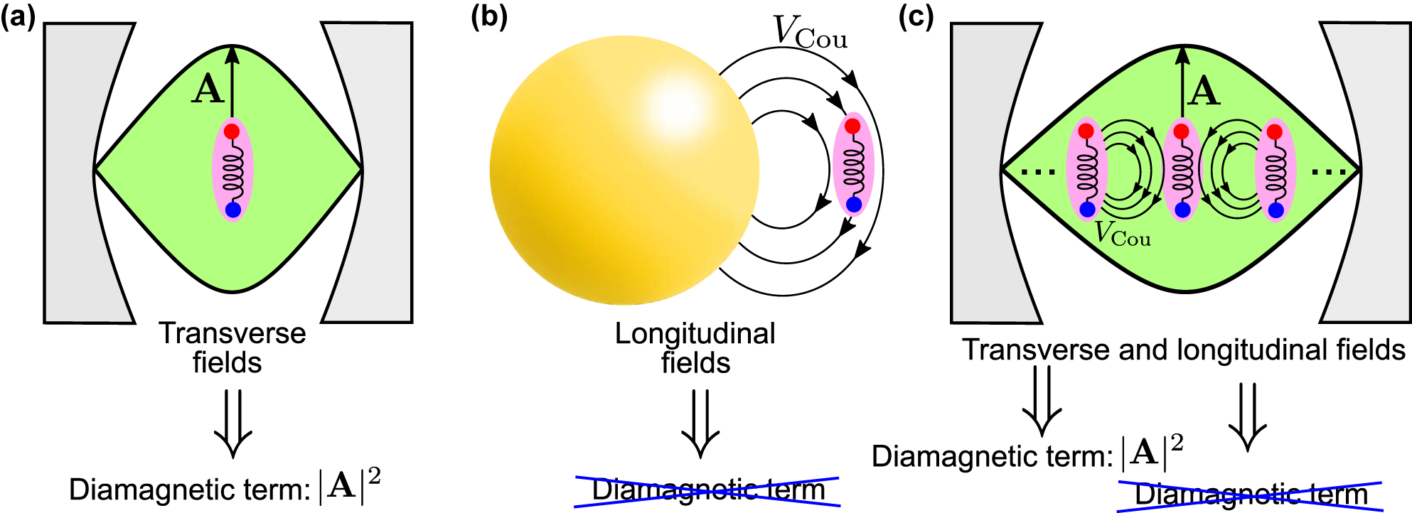
Schematics of the interaction between matter excitations and cavity modes in the three systems considered in this work. (a) A molecular emitter (as a representative quantum emitter) placed inside a dielectric (Fabry–Pérot) cavity. The transverse field of the single cavity mode considered is described with the vector potential A, which leads to the presence of the diamagnetic term ∝|A|2 in the cavity-QED Hamiltonian that describes this system. (b) A molecular emitter close to a metallic spherical nanoparticle and coupled to a single plasmonic mode. Within the quasistatic approximation, the molecular emitter only interacts with the longitudinal fields of the spherical nanoparticle, via the Coulomb potential V Cou. Since the vector potential A is not considered, the diamagnetic term is absent in the corresponding cavity-QED description. (c) An ensemble of molecular emitters placed inside a Fabry–Pérot cavity. The molecular emitters behave as a homogeneous bulk material. In this system, each emitter interacts with the transverse cavity mode characterized by the vector potential A as well as with the longitudinal fields associated with the Coulomb potential V Cou induced by the other molecular emitters. Whereas the interaction of each emitter with cavity modes requires a diamagnetic term in the cavity-QED description, the coupling with other emitters is described without this term.
2 Comparison of classical and cavity-QED models
In this section, we examine first a cavity-QED Hamiltonian that describes the interaction between a quantum emitter and a cavity optical mode. In Section 2.1, we derive the Heisenberg equations of motion for the displacements of the quantum operators, which take the form of classical oscillator equations. We present two equivalent descriptions, related by unitary transformations of the original quantum Hamiltonian. In one description, the coupling term between the oscillators is proportional to their amplitudes, while in the other, it is proportional to their time derivatives. Both approaches yield the same results, as the coupling strength and cavity frequency are appropriately renormalized in each case.
In nanophotonics, bare cavity frequencies, which can be measured or computed, are typically used when fitting experimental and simulated spectra, without considering their potential renormalization. We, therefore, focus on classical models with un-renormalized cavity frequencies, referring to them as the Spring Coupling (SpC) model for amplitude-based coupling, and the Momentum Coupling (MoC) model for coupling based on time derivatives of the amplitudes.
For specific values of the diamagnetic term in the Hamiltonian, the Heisenberg equations align naturally with either the SpC (Section 2.2) or MoC (Section 2.3) models, making each of them the most appropriate choice for fitting different experimental data. Section 2.4 illustrates the differences between these two models.
2.1 Derivation of the classical models from the Hamiltonians
In this subsection, we introduce the classical harmonic oscillator models. To this purpose, we first analyze the light–matter interaction using the cavity-QED framework. The cavity modes and the matter excitations are quantized using bosonic operators. The use of bosonic operators is valid for the cavity modes, and for matter excitations such as vibrations or phonons associated with a potential with a harmonic dependence on the degrees of freedom. The correspondence with classical harmonic oscillators (and thus the use of bosonic operators) is also valid to treat the coupling with matter excitations of fermionic nature provided that the number of excitations is much smaller than the number of quantum emitters (molecules, quantum dots…) and that any other effects induced by the saturation of the fermionic states can be discarded. Under these conditions, for example, the Quantum Rabi model (a generalization of the Jaynes–Cummings model to the ultrastrong coupling regime that includes a fermionic excitation [21]) becomes analogous to an appropriate bosonic Hamiltonian with a single matter excitation. Under this prescription based on bosonic operators, we can use a Hopfield-type Hamiltonian [48] in the form
as shown in the Supplementary Material. In this Hamiltonian, the creation operator
From the Hopfield Hamiltonian, we can obtain the equations of motion of the displacements (or oscillation amplitudes) of two quantum oscillators. With this aim, we connect the creation and annihilation operators from the Hamiltonian in Eq. (1) with the quantum operators
These are not the only classical equations that could describe the spectra of the coupled system. Any Hamiltonian
where the prime ′ denotes that the matter operators are transformed (
In this new reference frame, we can calculate the equations of motion for the expectation values
We find that, in contrast to Eq. (2), the coupling term is now proportional to the time derivative of the oscillation amplitudes.
To obtain the classical harmonic oscillator models, it is just necessary to associate the expectation values of the quantum operators to classical oscillation amplitudes, e.g.,
and Eq. (5) becomes
where we do not make an explicit distinction between
Importantly, once the different interpretation of
Thus, it is always possible to obtain the optical response of the coupled system by considering the coupling to be proportional to either the oscillation amplitudes or their time derivatives. An important point to notice is that, in both Eqs. (6b) and (7b), the “matter resonant frequency” (square root of the term proportional to x
mat) is the bare frequency ω
mat. However, the “cavity resonant frequency” (square root of the term proportional to x
cav) is different in the different oscillator models. In the model characterized by Eq. (6a), the shifted cavity frequency is
In nanophotonics, coupled harmonic oscillator equations have been widely used to fit data without considering frequency renormalization so we adhere to this procedure, i.e., we consider harmonic oscillator models where the frequency of the cavity and matter excitations are the bare ones. This approach gives preference to the model with coupling constant proportional to the oscillation amplitude (Eq. (6)) or to its derivative (Eq. (7)), depending on the value of D, as discussed next. Thus, throughout the remaining of this paper (including the Supplementary Material unless otherwise stated), we analyze these two preferred models using bare frequencies. We denote these models the Spring Coupling (SpC) model and the Momentum Coupling (MoC) model, respectively. Other models are discussed in Section S2 and summarized in Section S4 of the Supplementary Material. Additionally, Section S1 of the Supplementary Material details how to obtain the classical coupled harmonic oscillator equations directly from the classical electromagnetic Lagrangian.
2.2 Spring Coupling (SpC) model
We consider first a system without diamagnetic term, D = 0. This choice is appropriate, for example, when the interaction between the emitter and cavity excitations is mediated by Coulomb coupling, as discussed in more detail in Section 3.2. Eq. (6) then becomes
where the coupling is proportional to the classical oscillation amplitudes x
cav and x
mat and we have changed the notation g
SpC = g
QED (using a different symbol for the coupling strength in the classical and quantum descriptions becomes useful in Section 2.3). The
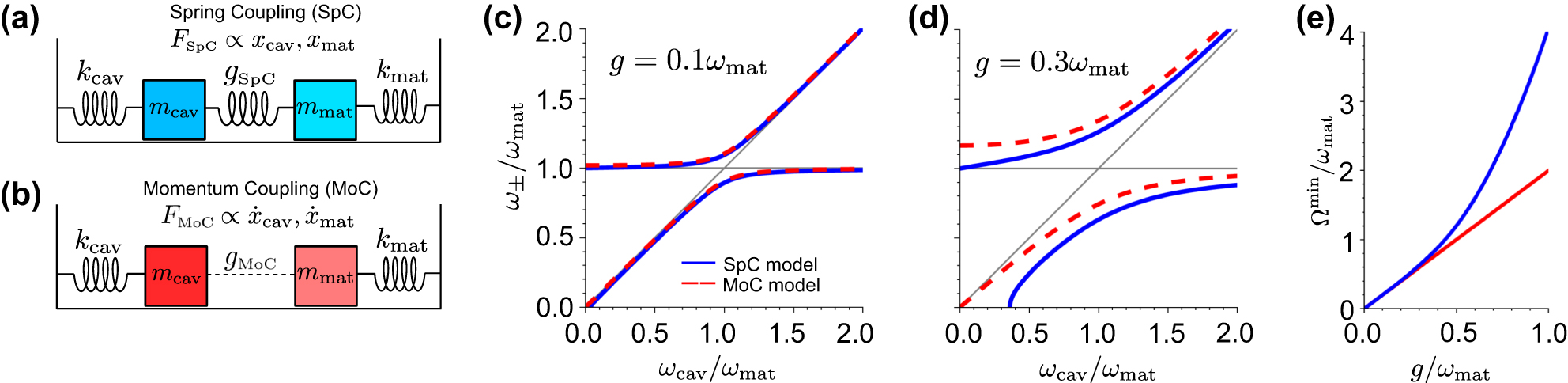
We refer to Eqs. (8) and (9) as the Spring Coupling (SpC) model because they are analogous to the equations describing the movement of two coupled springs (sketch in Figure 2(a)) (we emphasize that we could also describe the same physics of ultrastrongly coupled systems by setting D = 0 in Eq. (7), but, in this case, the dressed frequency
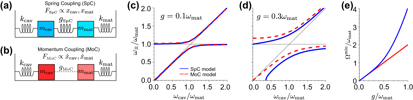
Comparison of the Spring Coupling (SpC) and Momentum Coupling (MoC) models. (a) Schematics of the SpC model in analogy to an oscillator model in classical mechanics. The coupling mechanism of strength g
SpC is analogous to a force F
SpC exerted by a spring and proportional to the oscillator displacements x
cav and x
mat. (b) Schematics of the MoC model. The coupling mechanism of strength g
MoC is analogous to a force F
MoC proportional to the time derivatives of the oscillator displacements
We note that frequencies given by Eq. (10) correspond to the energy difference between the first excited and ground state, and not to the absolute values of the eigenfrequencies themselves. This distinction is not necessary in classical descriptions that set the energy of the ground state to zero (or a fixed value). However, the cavity-QED model indicates a g
QED-dependent shift of the ground-state energy from zero, which is a fully quantum phenomenon. The information of this shift is lost when we take the expectation value of the operators
2.3 Momentum Coupling (MoC) model
For a diamagnetic term with
with the coupling term proportional to the time derivative of the oscillation amplitudes (the “velocities”) so that we call this model the Momentum Coupling (MoC) model (sketch in Figure 2(b)). The coupling strength g
MoC in these equations is related to the constant g
QED in the cavity-QED Hamiltonian as
and the corresponding eigenfrequencies are
Although the MoC is used to describe the coupling between matter excitations and cavity modes (Figure 2(b)), we are not aware of any equivalent mechanical system in classical mechanics that follows the equations of motion in Eqs. (11a) and (11b) (with coupling terms proportional to the time derivatives of the oscillation amplitude, similarly to friction terms but describing the interaction between two different oscillators). This is in contrast to the SpC model where the equivalent system, composed of masses and springs, is shown in Figure 2(a).
2.4 Comparison of the MoC and SpC models
As mentioned above, the MoC and SpC models are appropriate when
The MoC and SpC models are known to give very different results for g ≫ 0.1ω mat, as we briefly illustrate in this section (we use g in this subsection to refer to g SpC or g MoC in discussions that are valid for both models). Figure 2(c) compares the eigenfrequencies of the SpC (blue solid line) and MoC (red dashed line) models for g = 0.1ω mat, as given by Eqs. (10) and (13), respectively. For simplicity, we consider that the coupling strength is the same for all values of ω cav (a different parameter choice is discussed in Section S6 of the Supplementary Material). The eigenfrequencies of the hybrid modes ω ± are calculated as a function of the bare cavity frequency ω cav, with the bare ω mat frequency fixed (all frequencies are normalized by ω mat, so that the figures are independent of the value of this parameter). The eigenfrequencies obtained within the MoC and SpC models follow a nearly identical dependence on ω cav, and the agreement is even better for g < 0.1 ω mat. Thus, when analyzing systems not in the ultrastrong coupling regime, the two models can generally be used interchangeably with minimal impact on the results, although exceptions can exist [60].
In contrast, the choice of the model is crucial for even larger coupling strengths, such that the system is well into the ultrastrong coupling regime. The differences between the two models are illustrated in Figure 2(d) for coupling strength g = 0.3 ω
mat. In this case, the two models predict significantly different eigenfrequencies of the coupled system. The difference is smaller for larger cavity frequencies, ω
cav ≫ ω
mat, because the oscillators become uncoupled and the eigenfrequencies approach the bare frequencies ω
cav and ω
mat in the two models. However, even for a relatively large
We compare next the splitting Ω = ω + − ω − between the two eigenmodes at zero detuning, ω cav = ω mat. In the MoC model, the splitting equals twice the coupling strength, i.e., Ω = 2g, which is the minimum splitting in this model [61], [62]. On the other hand, in the SpC model, the relation between Ω and the coupling strength for zero detuning is
We find ΩSpC = 2.11g
SpC for the values used in Figure 2(d). Further, according to the SpC model, the minimum splitting between the branches does not happen at zero detuning but at cavity frequencies larger than the matter excitation frequencies. To further emphasize the difference between the models, Figure 2(e) shows the minimum splitting as a function of coupling strength, with a linear dependence for the MoC (red solid line) model, Ωmin = 2g, in contrast with the strong deviation from nonlinearity of the SpC model results (blue line) for g ≫ 0.1ω
mat. As a consequence, close to the so-called deep strong coupling regime
Last, Figure 2(d) shows important differences at small cavity frequencies, ω
cav ≪ ω
mat. The dispersion of the MoC model shows two hybrid modes for all values of the detuning, with the lower mode frequency ω
−,MoC tending toward ω
cav for decreasing value of ω
cav. In contrast, for the SpC model, the lower mode ceases to exist (ω
−,SpC becomes imaginary) under the condition
The two models’ different asymptotic limits of the upper branch determine the predicted range of energies where hybrid modes can exist. The MoC results show a frequency band between ω
mat and
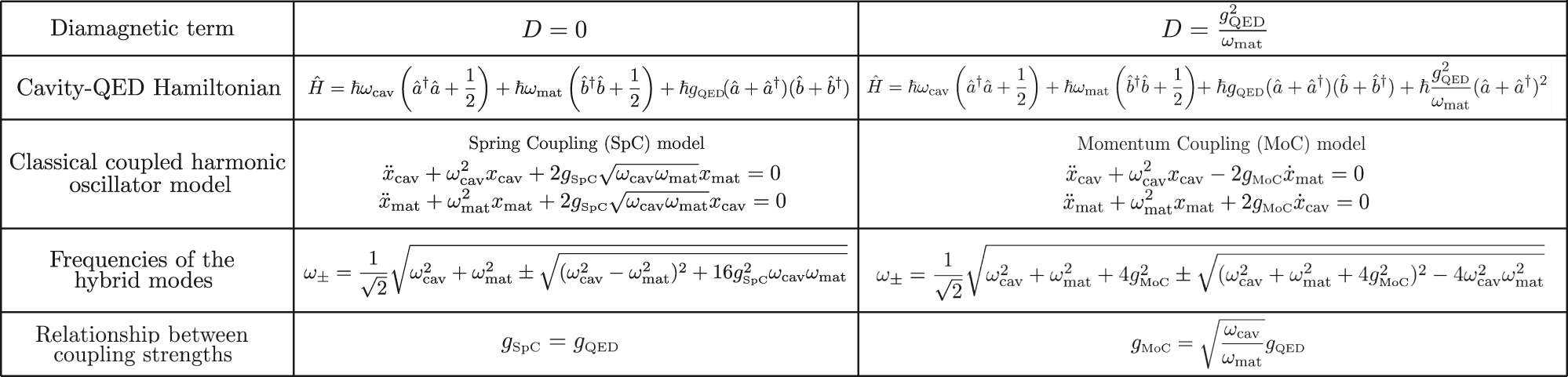
The connection between classical and quantum models is summarized in Table 1. The classical SpC and MoC models result in the same eigenfrequencies as cavity-QED Hamiltonians without the diamagnetic term (D = 0) and with
Summary of the correspondences of the classical SpC and MoC models with the cavity-QED description without diamagnetic term D = 0 (second column) and with diamagnetic term and
 |
At this point, we have discussed the connections between a general quantum description and classical equations of motion. However, we still need to determine how to choose between the MoC and SpC models for a given system (or equivalently, whether the Hamiltonian has D ≠ 0 or D = 0). In the next section, we consider three representative systems to explore this question and highlight the key role played by the nature of the matter–cavity interaction (Coulomb coupling or coupling with transverse electromagnetic modes in dielectric cavities).
Additionally, we have focused thus far on the eigenfrequencies, which can be extracted directly from the equations of coupled harmonic oscillators without needing an exact understanding of what the oscillation amplitudes x cav and x mat represent. However, a clear physical interpretation of these parameters is necessary to evaluate magnitudes of interest, such as the electric field at a given location inside or outside the optical cavity. In Section 3, we also address how x cav and x mat relate to relevant physical quantities in the representative systems of choice.
3 Physical observables from classical models in configurations of interest
We analyze in this section the three canonical nanophotonics systems introduced in Figure 1, for which different cavity-QED Hamiltonians (with and without the diamagnetic term) are appropriate. In Section 3.1, we focus on the textbook case of a single molecular emitter (or another quantum emitter) interacting with transverse electromagnetic modes of the dielectric Fabry–Pérot cavity in Figure 1(a) (in transverse modes, the fields are perpendicular to the wavevector in all Fourier components). As a second example, we analyze in Section 3.2 a molecular emitter close to a small metallic nanoparticle (Figure 1(b)), where the coupling is governed by Coulomb interactions (the fields mediating this interaction are longitudinal, i.e., parallel to the wavevector in all Fourier components). The last example (Section 3.3) consists of an ensemble of molecular emitters (representing a bulk material) inside a Fabry–Pérot cavity (Figure 1(c)), where the molecules couple with a transverse electromagnetic mode of the cavity and also interact with each other through Coulomb coupling.
3.1 A quantum emitter interacting with a transverse mode of a dielectric cavity
We consider first a dipole interacting with a single transverse mode of a resonant dielectric cavity (Figures 1(a) and 3(a)). The dipole is associated with matter excitations, and it can represent an excitonic transition of a molecule or quantum dot or a transition between vibrational states, for example. For concreteness, we consider the coupling with a molecular emitter in the following. Cavity-QED models of this system have successfully described phenomena such as the modification of the spontaneous emission rate of the emitter [63], [64], of the photon statistics of the emitted light [60], [65], [66], or of the coherence time of the quantum states [67].
Interaction of a quantum emitter with a transverse cavity mode within the classical MoC model. (a) Schematics of the system. The two oscillators are associated with the vector potential A of the cavity mode and the induced dipole moment d of the excitation in the quantum emitter, which we consider to be a molecule. The oscillators are coupled with each other with strength g
MoC. The bottom sketch indicates the cavity dimensions that we analyze in the rest of the panels. The emitter is placed at the center of the cavity. The green shaded areas in the sketches represent the field distribution of the cavity mode. (b) Spatial distribution of the electric field for the upper (blue) and the lower (red) hybrid modes at frequencies ω
+,MoC and ω
−,MoC, respectively, for coupling strength g
MoC = 2.5 ⋅ 10−4
ω
cav. The electric field is calculated along the cavity axis (along the x direction in panel (a), with x = y = z = 0 corresponding to the cavity center). The inset is a zoom of the region near the emitter. (c) Contribution to the electric field from the cavity
The whole derivation of the equations of motion of the classical variables within the Coulomb gauge is discussed in the Supplementary Material (Section S1), but we summarize it in the following. We represent the molecular emitter as two point charges with relative position l (forming a dipole), which couple through Coulomb interactions determined by the potential V
Cou(l) approximated as a harmonic one,
In cavity-QED models, the standard approach to describe light–matter interactions in this system is to use the minimal-coupling classical Hamiltonian in the Coulomb gauge of the form
where
Comparing this expression with the third term of the Hopfield Hamiltonian (Eq. (3)), we directly obtain that the coupling strength in the cavity-QED formalism is
Next, we use the connection between the classical and cavity-QED approaches to illustrate the procedure to obtain the value of physical observables from the classical oscillation amplitudes of the cavity x
cav and of the molecular excitation x
mat. The classical coupling strength g
MoC is directly obtained from the quantum value as
where, for an appropriate comparison between classical amplitudes and quantum operators, the real part of the oscillator amplitudes must be taken: Re(x
cav) = Re(|x
cav|e−iωt+ϕ
) ∝|x
cav| cos(ωt + ϕ), with ϕ a phase. Equations (20a) and (15) indicate that the oscillation amplitude x
cav in the MoC model (Eq. (11)) is given by
We are finally in conditions to obtain the value of physical observables such as the electric field from the classical harmonic MoC model. We first consider the spatial distribution of the electric fields of each hybrid mode. The transverse cavity mode field (given by A(r, t)) must be added to the longitudinal near field induced by the induced dipole,[1] which is obtained from the scalar Coulomb potential
with unit vectors
and the electric field at frequencies ω ±,MoC of each hybrid mode (given by Eq. (13)) corresponds to
with
Inserting Eq. (24) into (23), we obtain the ratio between the contributions of the cavity electric field and the matter excitation.
Equations (23) and (24) are a main result of this subsection and can be used to obtain the electric field at any position and for an arbitrary transverse mode with field distribution given by Ξ(r). We consider for illustration the particular case of a molecule (as an example of quantum emitter) introduced in the center of a dielectric cavity consisting in a rectangular vacuum box enclosed in the three dimensions by perfect mirrors, as sketched in Figure 3(a). The cross-section of the box is square, with size L x = L y = 292 nm and its height is L z = 215 nm, which results in a fundamental lowest-order cavity mode at frequency ω cav = 3 eV and an effective volume V eff = 4.483 ⋅ 106 nm3 (for an easier comparison between classical frequencies ω and quantum energies ℏω, in this paper, we use eV as a unit for both of them). This value of V eff is calculated from the general expression of dielectric structures [70]
where ɛ(r) refers to the permittivity of the system at position r, and in this particular case, we consider ɛ(r) = 1 inside the cavity. The molecular excitation is nearly resonant with the cavity, ω
mat ≈ ω
cav = 3 eV, but its exact frequency is changed to study the effects of detuning. The transition dipole moment
We show in Figure 3(b) the distribution of the z component of the electric field inside this cavity for the upper hybrid mode E
z
(x, ω
+,MoC) and for the lower hybrid mode E
z
(x, ω
−,MoC), as obtained from Eq. (23). We plot the fields as a function of the position in the x direction with respect to the location of the molecular emitter at the center of the cavity. To highlight the differences between the contributions of the cavity and the induced dipole in the two modes, we choose a slight detuning of ω
cav − ω
mat = 1.5 meV. Since the classical MoC model does not give the absolute value of the eigenmode fields, we choose arbitrary units so that the contribution of the cavity mode to the electric field of the upper hybrid mode (E
cav(r, ω
+,MoC) in Eq. (23)) has a maximum absolute value of 1. This choice fixes all the other values according to Eq. (24).[2] The fields are dominated by the cavity mode far from the cavity center and by the contribution from the molecular dipole close to x = 0. The field distribution shows a clear difference in the behavior of the two hybrid modes. For the upper mode, the induced dipole points in the same direction as the cavity field
Further, Eqs. (23) and (24) also enable to examine the dependence of the field E(r, ω
±,MoC) inside the cavity with detuning ω
mat − ω
cav. Figure 3(c) shows the contributions to this electric field of the cavity and the molecular emitter for each hybrid mode, normalized with respect to the sum of both contributions, according to
The coupling strength we have considered in this subsection corresponds to the strong coupling regime (we have neglected losses) but is far from the ultrastrong coupling regime so that the phenomena studied can also be explained with the classical linearized model (Section S5 of the Supplementary Material). On the other hand, we consider again in Figure 3(d) the contributions to the electric field
The described methodology thus enables obtaining results equivalent to those of the cavity-QED description (Hopfield Hamiltonian with the diamagnetic term) by using an intuitive classical model of coupled harmonic oscillators. In summary, we have shown in this section how to use the classical MoC model to characterize the fields in a hybrid system composed of a molecular emitter coupled to a transverse mode of a cavity.
3.2 A quantum emitter interacting with the longitudinal field of a metallic nanoparticle through Coulomb coupling
Next, we consider a quantum emitter placed close to a metallic nanoparticle to analyze how to model an alternative system and obtain physical observables in the strong and ultrastrong coupling regimes. These nanoparticles are attractive in nanophotonics because they support localized surface plasmon modes characterized by very low effective volumes [18], [71], [72], [73], [74]. Since the coupling strength is inversely proportional to the square root of the effective mode volume, very large coupling strengths can be obtained even when the nanoparticle interacts with a single molecule or quantum dot. We consider again a molecule as a representative quantum emitter.
In order to analyze the interaction of the dipolar plasmonic mode of the nanoparticle with a molecular (harmonic) excitation of dipole moment d mat, we consider that the size of the nanoparticle and the molecule-nanoparticle distance are much smaller than the light wavelength and treat the system within the quasistatic approximation. Under this approximation, the temporal variation of the vector potential A in Eq. (22) is negligible. Therefore, the coupling between the nanoparticle and the molecular emitter is governed by Coulomb interactions expressed by a scalar potential V Cou. The coupling is then mediated by longitudinal fields, in contrast to the coupling with transverse fields in Section 3.1.
In this context, the emitter-nanoparticle coupling cannot be modeled with the minimal coupling Hamiltonian as in Section 3.1, and it is described instead through the interaction Hamiltonian [75]
We insert the quantized expressions of the induced dipole moments
with coupling strength
where we have defined the unit vectors as
The representation of the plasmon-molecule system with the SpC model is schematically shown in Figure 4(a). To obtain the observables in this system, we use the equivalence of the oscillation amplitudes x
cav and x
mat with the induced dipole moments of the cavity and the molecular (or matter) excitation. This equivalence can be obtained from Eqs. (17) and (20), and it follows
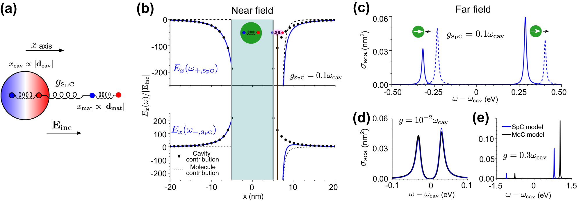
Modeling of the coupling between a quantum emitter and a metallic spherical nanoparticle (a plasmonic nanocavity) within the classical SpC model. (a) Schematics of the system. The quantum emitter is considered to be a molecule. The molecular excitation (of induced dipole moment d
mat) and the dipolar mode of the plasmonic nanocavity (of induced dipole moment d
cav) are described as two harmonic oscillators (of oscillation amplitudes x
mat and x
cav) that are coupled with strength g
SpC. The system is excited by a laser of electric field amplitude E
inc. The radius of the spherical nanoparticle is 5 nm, and the molecular emitter is placed at a 1 nm distance from the nanoparticle surface along the x axis (the center of the nanoparticle corresponds to x = y = z = 0). d
cav, d
mat, and E
inc are polarized along x. (b) Electric field distribution along the x axis (y = z = 0) when the system is excited at the frequency of the upper hybrid mode ω
+,SpC (top panel) and of the lower hybrid mode ω
−,SpC (bottom panel). The fields are real and are evaluated only outside the nanocavity, with the positions inside highlighted by the green-shaded area. The position of the molecular emitter is indicated by the vertical brown line. We evaluate the fields for coupling strength g
SpC = 0.1 ω
cav, and ω
cav = ω
mat = 3 eV. For each hybrid mode, the cavity contribution to the field is indicated by dots, the contribution from the emitter by dashed lines, and the total field by blue solid lines. (c) Scattering cross section of the same system, with g
SpC = 0.1 ω
cav, as a function of the detuning of the laser ω − ω
cav. Solid lines: tuned system with frequencies ω
cav = ω
mat = 3 eV. Dashed lines: detuned system with frequencies ω
cav = 3 eV and ω
mat = 3.2 eV. (d) Scattering cross section of the tuned system (ω
cav = ω
mat = 3 eV), comparing the result of the SpC model (blue line) to the results of the MoC model (black line), in the strong coupling regime, g = 10−2
ω
cav. (e) Same as in (d) for the ultrastrong coupling regime, g = 0.3 ω
cav. In all results f
cav = (4345e)2/m
p (where m
p is the mass of the proton),
We consider next that the dipolar mode of the metallic nanoparticle is illuminated by an external field of amplitude E
inc and frequency ω. We introduce this field in the SpC model as a forcing term that acts both onto the nanoparticle and onto the molecular emitter. Specifically, this is done by adding terms
These expressions are consistent with an alternative classical model that describes the nanocavity and the molecular emitter as dipolar polarizable objects (Section S1 of the Supplementary Material), supporting the validity of the general approach presented here. In the absence of losses [49], the induced dipole moments d
cav and d
mat diverge at the eigenfrequencies ω
±,SpC of the SpC model (Eq. (10)). To avoid these divergences, we add an imaginary part to the bare cavity and matter frequencies in this section. These imaginary parts are related to the decay rates of the cavity, κ, and of the matter excitation, γ, as
As an example, we consider a metallic spherical nanoparticle of radius R
cav = 5 nm and with a cavity mode of frequency ω
cav = 3 eV. We consider the same molecular emitter of Section 3.1, with a strong transition dipole moment of magnitude μ
mat = 15 Debye. As indicated by Eq. (28), the coupling strength of the system can be adjusted based on the position and orientation of the molecular emitter. We choose that the dipolar molecular transition is polarized perpendicularly to the surface of the nanoparticle and parallel to the amplitude of the incident field E
inc, to maximize the coupling strength (as a consequence d
cav, d
mat,
The induced dipole moments obtained from Eq. (29) can be used, for example, to calculate the near-field distribution under excitation at frequency ω. The total electric field is the sum of the cavity
From this expression, the fields at the frequency of each hybrid mode are calculated by replacing into Eq. (30) the oscillation amplitudes in Eq. (29) induced at the mode frequencies ω ±,SpC.
The electric fields along the x-axis associated with the upper and lower mode frequencies are plotted in the top and bottom panels of Figure 4(b) (blue lines), respectively. These fields are real and polarized along the x direction. We further show the decomposition of the fields into the contribution of the cavity (black dots) and the molecular emitter (black dashed line) as given by the first and second terms on the right-hand side of Eq. (30), respectively. It can be appreciated from Figure 4(b) that, for example, when the upper hybrid mode is excited, the dipoles associated with the cavity and the molecular emitter are oriented in the same direction (same sign). In contrast, for the lower mode, the dipoles point toward the opposite direction.
The near field plotted in Figure 4(b) is useful for analyzing the behavior of the hybrid modes. Still, it is difficult to measure, and most experiments focus on far-field spectral information, such as in the scattering cross section spectral σ sca. Due to the small emitter-nanocavity distance, we neglect retardation effects so that σ sca is related to the total induced dipole moment of the system as [78]
We show in Figure 4(c) the scattering cross section for the same nanoparticle-molecular emitter system in the outset of the ultrastrong coupling regime (g SpC = 0.1 ω cav). Since the oscillator strength of the cavity is much larger than that of the emitter (f cav ≫ f mat), the spectrum is entirely dominated by the cavity contribution, obtained from Eq. (29a) (however, in other systems, where both oscillator strengths are similar, f cav ≈ f mat, it is crucial to consider both contributions in Eq. (31)). The scattering cross section spectra are shown for two different detunings between the nanocavity and the molecular emitter. At zero detuning (ω cav = ω mat = 3 eV, solid lines in Figure 4(c)) the upper hybrid mode has a (moderately) larger cross section than the lower hybrid mode, mostly due to the ω 4 factor in Eq. (31). However, when the molecular excitation is blue detuned with respect to the cavity (ω cav = 3 eV and ω mat = 3.2 eV, dashed line), the strength of the peak in the cross section spectra associated with the lower hybrid mode increases and the upper hybrid mode becomes weaker. This behavior occurs because, for this detuning, the lower hybrid mode acquires a larger contribution of the cavity resonance that dominates the scattering spectra, while the predominantly emitter-like behavior of the upper mode results in a smaller cross section due to f mat ≪ f cav.
To assess the importance of using the classical SpC model to describe this system, we compare the results of the scattering cross section spectra calculated with this model with those obtained using the MoC model. For this purpose, it is necessary to obtain the expressions of the scattering cross section for the latter model under external illumination. By introducing forcing terms in the equations of motion of the MoC model (Eq. (11)) to account for the external field, we obtain the corresponding oscillation amplitudes
We calculate the scattering cross section according to each classical model by introducing these oscillations amplitudes in Eq. (31). Figure 4(d) shows the spectra for the system at zero detuning (ω cav = ω mat = 3 eV) in the strong coupling regime but far from the ultrastrong coupling regime, with g = 10−2 ω cav. As expected, the spectra calculated from the two models overlap almost perfectly (black line: MoC model; blue line: SpC model). The difference between the two calculations is less than 10 % at the hybrid mode frequencies ω ±. This small error is consistent with the good agreement of the eigenfrequencies in Section 2 for this relatively low value of g.
In contrast, if the system is well into the ultrastrong coupling regime, with coupling strength g = 0.3 ω cav, the spectra obtained with the two models are very different (Figure 4(e)). There is a clear disagreement in the peak positions due to the difference in the eigenfrequencies of the two models (see Figure 2(d)). Further, the MoC model predicts that the strength of the peak corresponding to the excitation of the upper hybrid mode is twice larger than the equivalent value from the SpC model. These significant differences emphasize the importance of the choice of the model in this regime. However, we note that for such large coupling, higher-order modes of the nanocavity are likely to play an important role in the coupling, which would need to be considered in realistic systems [79]. Further, examining how this analysis is modified when going beyond the quasistatic description would be of interest.
3.3 An ensemble of interacting molecules in a Fabry–Pérot cavity
The previous two examples illustrate the procedure for connecting the variables in the SpC and MoC models to physical observables. In both cases, the optical cavity was coupled to a single quantum emitter, a very challenging situation for experimentally reaching the ultrastrong coupling regime. An alternative approach to access the necessary coupling strengths consists in filling a cavity with many molecules or with a material supporting a well-defined excitation (such as a phononic resonance) [54], [80], [81]. We consider in this section a homogeneous ensemble of molecular emitters as the material that interacts with resonant transverse electromagnetic modes of a Fabry–Pérot cavity (left sketch in Figure 5(a)), a system of significant relevance in experiments [5], [46], [82], [83]. Each molecule presents a vibrational excitation that is modeled as a dipole of induced dipole moment d i (we focus here on the case of molecular emitters for specificity, but the same derivation can also be applied to phononic or similar materials by focusing on the induced dipole moment associated to each unit cell). We consider that all molecular emitters are identical and thus have the same oscillator strength f dip and resonant frequency ω dip. We use the subindex dip to emphasize that, at this stage, we are considering the individual molecular dipoles and not the whole material (the full ensemble of molecular emitters) involved in the coupling. For simplicity, we assume that there are N dip molecular emitters distributed homogeneously. The electromagnetic modes of the Fabry–Pérot cavity are standing waves with vector potential A α and frequency ω cav,α , where all α modes are orthogonal.

Interaction between matter excitations within a homogeneous material and the transverse modes of a dielectric cavity. (a) (Left) Schematic of the system. The homogeneous material is modeled as an ensemble of dipolar molecular emitters with a vibration at frequency ω
dip,i
. The oscillators x
cav,α
represent the vector potential A
α
associated with all modes α in the cavity, and the individual matter oscillators x
dip,i
represent the induced dipole moments d
i
of each molecular emitter. The cavity–molecular emitter interactions are modeled with the MoC model and coupling strength
Following the relations between the observables and oscillators given in Section 3.1, we represent each vibrational dipole as a harmonic oscillator with oscillation amplitude
where the sum extends over all cavity modes (∑ α ) and molecular emitters (∑ i and ∑ j ).
The direct calculation of the dynamics of the entire system requires solving N dip × N cav equations, where N cav is the number of cavity modes. However, due to the homogeneity of the material and the orthogonality of the cavity modes, each cavity mode α only couples with a collective matter excitation, which is represented by an oscillator of oscillation amplitude x mat,α ∝∑ i Ξ α (r i )x dip,i , i.e., the amplitude of the individual molecular oscillators in the collective mode α is weighted by the cavity mode field at the same position. x mat,α thus captures the response of the whole material formed by the ensemble of molecules, as highlighted by the use of the mat subindex. The motion of each cavity mode α and the associated collective mode can then be obtained by solving the following two coupled equations (see Section S7 in Supplementary Material for the full derivation and the value of the different parameters)
In these equations, g
shift is a parameter that depends on the values
In this description, each cavity mode α only couples to the collective molecular mode where the induced dipoles are polarized following the orientation and spatial distribution Ξ
α
(r) of the cavity mode field. This collective molecular mode thus has a total induced dipole moment
We have thus shown that the MoC model constitutes the proper description of the coupling between transverse cavity modes and collective matter excitations in homogeneous materials. We further confirm the validity of this model to describe the system by demonstrating that it allows for recovering the typical bulk permittivity of phononic materials or ensembles of molecules and that this cannot be captured by the SpC model. We first note that, according to recent work [54], [88], [89], the dispersion of the cavity–matter system is exactly the same as the bulk dispersion of the material. This enables to relate the spectrum of the MoC model with the bulk permittivity ɛ(ω) of the material in the following manner: the cavity modes of the bare cavity (without molecular emitters) follow the dispersion of free photons as ω
cav,α
= ck
α
, with c the light speed in vacuum and k
α
the wavevector that is determined by the length L
cav of the Fabry–Pérot cavity (for perfect mirrors) as k
α
= n
α
π/L
cav, for an integer n
α
and normal incidence. For the cavity filled with molecular emitters, the frequency of each cavity mode of wavevector k
α
is modified from ω
cav,α
to
By comparing Eq. (36) with the previous relation
Equation (37) is the same that was discussed by Hopfield [48] and can be compared with the permittivity of polar materials. The latter can often be described in a range of infrared frequencies as
where ω
TO and ω
LO are the frequencies of the transverse optical and longitudinal optical phonons, respectively [90]. Thus, the MoC model recovers the permittivity of a polar material or an ensemble of molecules, with the correspondences Ωmat = ω
TO and
which does not follow the standard form of the permittivity (Eq. (38)).
For comparison, we plot in Figure 5(b) the permittivities obtained with the MoC model (red solid line, Eq. (37)) and the SpC model (blue solid line, Eq. (39)), as a function of the normalized frequency ω/Ωmat, with G = 0.3 Ωmat. The distinct behavior of permittivity predicted by the two models becomes evident when comparing their Reststrahlen bands. The Reststrahlen band represents the frequency range where electromagnetic waves cannot propagate in the bulk material (and also correspond to the maximum polaritonic gap achievable through the coupling of matter excitations with optical modes in dielectric resonators [54], [91]). The Reststrahlen band is delimited in polar materials by the phonon frequencies ω
TO and ω
LO. The MoC model describes the Reststrahlen band appropriately, because the permittivity is negative in the range
In this subsection, we have focused on the coupling with (harmonic) vibrations and phonons. Still, the discussion holds validity for other dipolar matter excitations, independent of their physical origin, such as molecular excitons. The main difference between excitons and vibrations is that the former are two-level systems (fermionic transitions), which, when the number of coupled molecules is low enough, introduces many nonlinear effects not included in classical harmonic oscillator models. However, when many molecules are present, the collective excitation is bosonic according to the Holstein–Primakoff transformation [92]. Therefore, while the discussions in Sections 3.1 and 3.2 are valid for harmonic excitations or for obtaining properties such as eigenvalues and electric field distribution under weak illumination, the discussion in this subsection is applicable more broadly.
4 Conclusions
We have analyzed the application of classical coupled harmonic oscillator models to describe nanophotonic systems under ultrastrong coupling and the connection of these models with quantum descriptions. This study focuses on the two classical models typically used in this context, here referred to as the Spring Coupling (SpC) and Momentum Coupling (MoC) models, where the difference relies on whether the coupling term is proportional to the oscillation amplitudes (SpC model) or to their time derivatives (MoC model). The choice between these models typically does not have significant consequences in the weak and strong coupling regimes, where both can be approximated to the same linearized model (this approximation is discussed in the Supplementary Material and is equivalent to the rotating-wave approximation in quantum models). However, the SpC and MoC models result in very different eigenvalues in the ultrastrong coupling regime. We show that the SpC model describes light–matter coupling induced by Coulomb interactions, such as those governing the interaction between different quantum emitters and between quantum emitters and small plasmonic nanoparticles, and that this model results in the same eigenvalue spectra as the quantum Hopfield Hamiltonian without diamagnetic term. On the other hand, the MoC model reproduces the spectra of systems for which the diamagnetic term should be present in the Hamiltonian, corresponding to systems where matter excitations interact with transverse electromagnetic fields (for example, in conventional dielectric cavities). The SpC and MoC models thus result in the same spectra of ultrastrongly coupled nanophotonic systems as a cavity-QED description without and with diamagnetic term, respectively, but using a simpler framework. These two classical models consider the bare cavity and matter frequencies, but we generalize the discussion in the Supplementary Material (Section S2) to alternative models of classical oscillators. This generalized analysis indicates that dressing the frequencies allows us to transform coupled harmonic oscillator models where the coupling is proportional to the oscillation amplitudes to equivalent equations with coupling proportional to their time derivatives and vice versa.
Additionally, classical oscillator models are typically used to calculate the eigenvalues of the system, but we discuss how they also provide other experimentally measurable magnitudes in three canonical systems of nanophotonics. We first show that the MoC model can be applied to calculate the electric field distribution of the two hybrid modes of a dielectric cavity filled by a single quantum emitter. Next, we use the SpC model to calculate the near-field distribution and the far-field scattering spectra of a quantum emitter located near a metallic nanoparticle. Last, the two models are combined to consider an ensemble of molecules inside a dielectric cavity. The molecules interact with each other through Coulomb interactions (SpC model) and also with the transverse electromagnetic modes of the dielectric cavity (MoC model). In this case, we show that the system response can be obtained by considering that each transverse cavity mode interacts with a collective molecular excitation. The only effect of the molecule–molecule dipolar interactions is to modify the effective frequency of these collective excitations, and the MoC model describes the ultrastrong coupling between these collective excitations and the cavity modes. Interestingly, the MoC model enables to recover correctly the permittivity and bulk dispersion of the material filling the cavity, and thus also the Reststrahlen band observed in polar materials, which is not the case for the SpC model. Alternative coupled harmonic oscillator models of the bulk dispersion are discussed in Section S8 of the Supplementary Material. Our work hence advances the exploration of classical descriptions of the ultrastrong coupling regime. It opens the possibility of simplifying the analysis of a wide variety of complex systems often described with quantum models.
Funding source: Ministerio de Ciencia, Innovación y Universidades MICIU
Award Identifier / Grant number: CEX2020-001038-M
Award Identifier / Grant number: CEX2023-001286-S
Award Identifier / Grant number: PID2020-115221GB-C41
Award Identifier / Grant number: PID2021-123949OB-I00
Award Identifier / Grant number: PID2022-139579NB-I00
Funding source: European Regional Development Fund
Award Identifier / Grant number: PID2021-123949OB-I00
Award Identifier / Grant number: PID2022-139579NB-I00
Funding source: Gobierno de Aragón
Award Identifier / Grant number: Q-MAD
Funding source: Agencia Estatal de Investigación
Award Identifier / Grant number: CEX2020-001038-M
Award Identifier / Grant number: CEX2023-001286-S
Award Identifier / Grant number: PID2020-115221GB-C41
Award Identifier / Grant number: PID2021-123949OB-I00
Award Identifier / Grant number: PID2022-139579NB-I00
Funding source: Eusko Jaurlaritza
Award Identifier / Grant number: 4usmart Elkartek
Award Identifier / Grant number: IT 1526-22
-
Research funding: UM, JA, and RE acknowledge grant PID2022-139579NB-I00 funded by MICIU/AEI/10.13039/ 501100011033 and by ERDF, EU, as well as grant no. IT 1526-22 from the Basque Government for consolidated groups of the Basque University and project 4usmart Elkartek funded by the Department of Economy of the Basque Government. RH acknowledges Grant CEX2020-001038-M funded by MICIU/AEI/10.13039/501100011033 and Grant PID2021-123949OB-I00 funded by MICIU/AEI/10.13039/501100011033 and by ERDF/EU. LMM acknowledges projects PID2020-115221GB-C41 and CEX2023-001286-S (financed by MICIU/AEI/10.13039/501100011033) and the Government of Aragon through Project Q-MAD.
-
Author contributions: UM derived the equations and performed the calculations in discussion with RE and JA. All authors contributed to the conception of the work, to the analysis of the results and to the writing of the manuscript. All authors have accepted responsibility for the entire content of this manuscript and approved its submission.
-
Conflict of interest: Authors state no conflict of interest.
-
Data availability: The datasets used to generate the figures in this paper are available in https://digital.csic.es/handle/10261/380579/.
References
[1] P. Törmä and W. L. Barnes, “Strong coupling between surface plasmon polaritons and emitters: a review,” Rep. Prog. Phys., vol. 78, no. 12, 2015, Art. no. 013901, https://doi.org/10.1088/0034-4885/78/1/013901.Search in Google Scholar PubMed
[2] D. S. Dovzhenko, S. V. Ryabchuk, Y. P. Rakovich, and I. R. Nabiev, “Light–matter interaction in the strong coupling regime: configurations, conditions, and applications,” Nanoscale, vol. 10, no. 8, pp. 3589–3605, 2018, https://doi.org/10.1039/c7nr06917k.Search in Google Scholar PubMed
[3] J. M. Fink, et al.., “Climbing the Jaynes-Cummings ladder and observing its n$\sqrt{n}$ nonlinearity in a cavity QED system,” Nature, vol. 454, no. 7202, pp. 315–318, 2008, https://doi.org/10.1038/nature07112.Search in Google Scholar PubMed
[4] R. Sáez-Blázquez, J. Feist, A. I. Fernández-Domínguez, and F. J. García-Vidal, “Enhancing photon correlations through plasmonic strong coupling,” Optica, vol. 4, no. 11, pp. 1363–1367, 2017, https://doi.org/10.1364/optica.4.001363.Search in Google Scholar
[5] A. Thomas, et al.., “Tilting a ground-state reactivity landscape by vibrational strong coupling,” Science, vol. 363, no. 6427, pp. 615–619, 2019, https://doi.org/10.1126/science.aau7742.Search in Google Scholar PubMed
[6] E. Orgiu, et al.., “Conductivity in organic semiconductors hybridized with the vacuum field,” Nat. Mater., vol. 14, no. 11, pp. 1123–1129, 2015, https://doi.org/10.1038/nmat4392.Search in Google Scholar PubMed
[7] G. Rempe, H. Walther, and N. Klein, “Observation of quantum collapse and revival in a one-atom maser,” Phys. Rev. Lett., vol. 58, no. 4, p. 353, 1987, https://doi.org/10.1103/physrevlett.58.353.Search in Google Scholar
[8] R. J. Thompson, G. Rempe, and H. J. Kimble, “Observation of normal-mode splitting for an atom in an optical cavity,” Phys. Rev. Lett., vol. 68, no. 8, p. 1132, 1992, https://doi.org/10.1103/physrevlett.68.1132.Search in Google Scholar PubMed
[9] Y. Kaluzny, P. Goy, M. Gross, J. M. Raimond, and S. Haroche, “Observation of self-induced Rabi oscillations in two-level atoms excited inside a resonant cavity: the ringing regime of superradiance,” Phys. Rev. Lett., vol. 51, no. 13, p. 1175, 1983, https://doi.org/10.1103/physrevlett.51.1175.Search in Google Scholar
[10] M. Brune, J. M. Raimond, P. Goy, L. Davidovich, and S. Haroche, “Realization of a two-photon maser oscillator,” Phys. Rev. Lett., vol. 59, no. 17, p. 1899, 1987, https://doi.org/10.1103/physrevlett.59.1899.Search in Google Scholar PubMed
[11] M. G. Raizen, R. J. Thompson, R. J. Brecha, H. J. Kimble, and H. J. Carmichael, “Normal-mode splitting and linewidth averaging for two-state atoms in an optical cavity,” Phys. Rev. Lett., vol. 63, no. 3, p. 240, 1989, https://doi.org/10.1103/physrevlett.63.240.Search in Google Scholar PubMed
[12] J. P. Reithmaier, et al.., “Strong coupling in a single quantum dot-semiconductor microcavity system,” Nature, vol. 432, no. 7014, pp. 197–200, 2004, https://doi.org/10.1038/nature02969.Search in Google Scholar PubMed
[13] S. Christopoulos, et al.., “Room-temperature polariton lasing in semiconductor microcavities,” Phys. Rev. Lett., vol. 98, no. 12, 2007, Art. no. 126405, https://doi.org/10.1103/physrevlett.98.126405.Search in Google Scholar
[14] A. Wallraff, et al.., “Strong coupling of a single photon to a superconducting qubit using circuit quantum electrodynamics,” Nature, vol. 431, no. 7005, pp. 162–167, 2004, https://doi.org/10.1038/nature02851.Search in Google Scholar PubMed
[15] N. S. Mueller, et al.., “Deep strong light–matter coupling in plasmonic nanoparticle crystals,” Nature, vol. 583, no. 7818, pp. 780–784, 2020, https://doi.org/10.1038/s41586-020-2508-1.Search in Google Scholar PubMed
[16] T. K. Hakala, et al.., “Vacuum Rabi splitting and strong-coupling dynamics for surface-plasmon polaritons and rhodamine 6G molecules,” Phys. Rev. Lett., vol. 103, no. 5, 2009, Art. no. 053602, https://doi.org/10.1103/physrevlett.103.053602.Search in Google Scholar PubMed
[17] P. Vasa, et al.., “Ultrafast manipulation of strong coupling in metal-molecular aggregate hybrid nanostructures,” ACS Nano, vol. 4, no. 12, pp. 7559–7565, 2010, https://doi.org/10.1021/nn101973p.Search in Google Scholar PubMed
[18] R. Chikkaraddy, et al.., “Single-molecule strong coupling at room temperature in plasmonic nanocavities,” Nature, vol. 535, no. 7610, pp. 127–130, 2016, https://doi.org/10.1038/nature17974.Search in Google Scholar PubMed PubMed Central
[19] J. Feist, J. Galego, and F. J. García-Vidal, “Polaritonic chemistry with organic molecules,” ACS Photonics, vol. 5, no. 1, pp. 205–216, 2018, https://doi.org/10.1021/acsphotonics.7b00680.Search in Google Scholar
[20] T. Niemczyk, et al.., “Circuit quantum electrodynamics in the ultrastrong-coupling regime,” Nat. Phys., vol. 6, no. 10, pp. 772–776, 2010.10.1038/nphys1730Search in Google Scholar
[21] A. F. Kockum, A. Miranowicz, S. De Liberato, S. Savasta, and F. Nori, “Ultrastrong coupling between light and matter,” Nat. Rev. Phys., vol. 1, no. 1, pp. 19–40, 2019, https://doi.org/10.1038/s42254-018-0006-2.Search in Google Scholar
[22] P. Forn-Díaz, L. Lamata, E. Rico, J. Kono, and E. Solano, “Ultrastrong coupling regimes of light-matter interaction,” Rev. Mod. Phys., vol. 91, no. 2, 2019, Art. no. 025005, https://doi.org/10.1103/revmodphys.91.025005.Search in Google Scholar
[23] C. Ciuti, G. Bastard, and I. Carusotto, “Quantum vacuum properties of the intersubband polariton field,” Phys. Rev. B, vol. 72, no. 11, 2005, Art. no. 115303, https://doi.org/10.1103/physrevb.72.115303.Search in Google Scholar
[24] K. Rzazewski, K. Wodkiewicz, and W. Zakowicz, “Phase transitions, two-level atoms and the A2 term,” Phys. Rev. Lett., vol. 35, no. 7, p. 432, 1975, https://doi.org/10.1103/physrevlett.35.432.Search in Google Scholar
[25] P. Nataf and C. Ciuti, “No-go theorem for superradiant quantum phase transitions in cavity QED and counter-example in circuit QED,” Nat. Commun., vol. 1, no. 1, p. 72, 2010, https://doi.org/10.1038/ncomms1069.Search in Google Scholar PubMed
[26] A. Vukics and P. Domokos, “Adequacy of the Dicke model in cavity QED: a counter-no-go statement,” Phys. Rev. A, vol. 86, no. 5, 2012, Art. no. 053807, https://doi.org/10.1103/physreva.86.053807.Search in Google Scholar
[27] T. Tufarelli, K. R. McEnergy, S. A. Maier, and M. S. Kim, “Signatures of the A2 term in ultrastrongly coupled oscillators,” Phys. Rev. A, vol. 91, no. 6, 2015, Art. no. 063840, https://doi.org/10.1103/physreva.91.063840.Search in Google Scholar
[28] D. De Bernardis, T. Jaako, and P. Rabl, “Cavity quantum electrodynamics in the nonperturbative regime,” Phys. Rev. A, vol. 97, no. 4, 2018, Art. no. 043820, https://doi.org/10.1103/physreva.97.043820.Search in Google Scholar
[29] C. Schäfer, M. Ruggenthaler, V. Rokaj, and A. Rubio, “Relevance of the quadratic diamagnetic and self-polarization terms in cavity quantum electrodynamics,” ACS Photonics, vol. 7, no. 4, pp. 975–990, 2020, https://doi.org/10.1021/acsphotonics.9b01649.Search in Google Scholar PubMed PubMed Central
[30] J. Galego, C. Climent, F. J. Garcia-Vidal, and J. Feist, “Cavity casimir-polder forces and their effects in ground-state chemical reactivity,” Phys. Rev. X, vol. 9, no. 2, 2019, Art. no. 021057, https://doi.org/10.1103/physrevx.9.021057.Search in Google Scholar
[31] J. Feist, A. I. Fernández-Domínguez, and F. J. García-Vidal, “Macroscopic QED for quantum nanophotonics: emitter-centered modes as a minimal basis for multiemitter problems,” Nanophotonics, vol. 10, no. 1, pp. 477–489, 2021, https://doi.org/10.1515/nanoph-2020-0451.Search in Google Scholar
[32] O. Di Stefano, et al.., “Resolution of gauge ambiguities in ultrastrong-coupling cavity quantum electrodynamics,” Nat. Phys., vol. 15, no. 2, pp. 803–808, 2019, https://doi.org/10.1038/s41567-019-0534-4.Search in Google Scholar
[33] W. Salmon, et al.., “Gauge-independent emission spectra and quantum correlations in the ultrastrong coupling regime of open system cavity-QED,” Nanophotonics, vol. 11, no. 8, pp. 1573–1590, 2022, https://doi.org/10.1515/nanoph-2021-0718.Search in Google Scholar PubMed PubMed Central
[34] L. Novotny, “Strong coupling, energy splitting, and level crossings: a classical perspective,” Am. J. Phys., vol. 78, no. 11, pp. 1199–1202, 2010, https://doi.org/10.1119/1.3471177.Search in Google Scholar
[35] S. R. K. Rodriguez, “Classical and quantum distinctions between weak and strong coupling,” Eur. J. Phys., vol. 37, no. 2, 2016, Art. no. 025802, https://doi.org/10.1088/0143-0807/37/2/025802.Search in Google Scholar
[36] S. Rudin and T. L. Reinecke, “Oscillator model for vacuum Rabi splitting in microcavities,” Phys. Rev. B, vol. 59, no. 15, 1999, Art. no. 10227, https://doi.org/10.1103/physrevb.59.10227.Search in Google Scholar
[37] A. B. Lockhart, A. Skinner, W. Newman, D. B. Steinwachs, and S. A. Hilbert, “An experimental demonstration of avoided crossings with masses on springs,” Am. J. Phys., vol. 86, no. 7, p. 526, 2018, https://doi.org/10.1119/1.5036752.Search in Google Scholar
[38] Y. S. Joe, A. M. Satanin, and C. S. Kim, “Classical analogy of Fano resonances,” Phys. Scr., vol. 74, no. 2, p. 259, 2006, https://doi.org/10.1088/0031-8949/74/2/020.Search in Google Scholar
[39] P. D. Hemmer and M. G. Prentiss, “Coupled-pendulum model of the stimulated resonance Raman effect,” J. Opt. Soc. Am. B, vol. 5, no. 8, pp. 1613–1623, 1988, https://doi.org/10.1364/josab.5.001613.Search in Google Scholar
[40] C. L. Garrido Alzar, M. A. G. Martinez, and P. Nussenzveig, “Classical analog of electromagnetically induced transparency,” Am. J. Phys., vol. 70, no. 1, pp. 37–41, 2002, https://doi.org/10.1119/1.1412644.Search in Google Scholar
[41] J. Harden, A. Joshi, and J. D. Serna, “Demonstration of double EIT using coupled harmonic oscillators and RLC circuits,” Eur. J. Phys., vol. 32, no. 2, pp. 541–558, 2011, https://doi.org/10.1088/0143-0807/32/2/025.Search in Google Scholar
[42] J. A. Souza, L. Cabral, R. R. Oliveira, and C. J. Villas-Boas, “Electromagnetically-induced-transparency-related phenomena and their mechanical analogs,” Phys. Rev. A, vol. 92, no. 2, 2015, Art. no. 023818, https://doi.org/10.1103/physreva.92.023818.Search in Google Scholar
[43] M. Harder and C.-M. Hu, “Chapter Two-Cavity spintronics: an early review of recent progress in the study of magnon-photon level repulsion,” Solid State Phys., vol. 69, pp. 47–121, 2018. https://www.sciencedirect.com/science/article/abs/pii/S0081194718300018.10.1016/bs.ssp.2018.08.001Search in Google Scholar
[44] X. Liu, et al.., “Strong light-matter coupling in two-dimensional atomic crystals,” Nat. Photonics, vol. 9, no. 1, pp. 30–34, 2015, https://doi.org/10.1038/nphoton.2014.304.Search in Google Scholar
[45] D. Yoo, et al.., “Ultrastrong plasmon-phonon coupling via epsilon-near-zero nanocavities,” Nat. Photonics, vol. 15, no. 2, pp. 125–130, 2021, https://doi.org/10.1038/s41566-020-00731-5.Search in Google Scholar
[46] J. George, et al.., “Multiple Rabi splittings under ultrastrong vibrational coupling,” Phys. Rev. Lett., vol. 117, no. 15, 2016, Art. no. 153601, https://doi.org/10.1103/physrevlett.117.153601.Search in Google Scholar PubMed
[47] A. V. Kats, M. L. Nesterov, and A. Y. Nikitin, “Excitation of surface plasmon-polaritons in metal films with double periodic modulation: anomalous optical effects,” Phys. Rev. B, vol. 76, no. 4, 2007, Art. no. 045413, https://doi.org/10.1103/physrevb.76.045413.Search in Google Scholar
[48] J. J. Hopfield, “Theory of the contribution of excitons to the complex dielectric constant of crystals,” Phys. Rev., vol. 112, no. 5, p. 1555, 1958, https://doi.org/10.1103/physrev.112.1555.Search in Google Scholar
[49] S. Hughes, C. Gustin, and F. Nori, “Reconciling quantum and classical spectral theories of ultrastrong coupling: role of cavity bath coupling and gauge corrections,” Opt. Quantum, vol. 2, no. 3, pp. 133–139, 2024, https://doi.org/10.1364/opticaq.519395.Search in Google Scholar
[50] D. Zueco and J. García-Ripoll, “Ultrastrongly dissipative quantum Rabi mode,” Phys. Rev. A, vol. 99, no. 1, 2019, Art. no. 013807, https://doi.org/10.1103/physreva.99.013807.Search in Google Scholar
[51] M. Autore, et al.., “Boron nitride nanoresonators for phonon-enhanced molecular vibrational spectroscopy at the strong coupling limit,” Light: Sci. Appl., vol. 7, no. 4, 2018, Art. no. 17172, https://doi.org/10.1038/lsa.2017.172.Search in Google Scholar PubMed PubMed Central
[52] N. Liu, et al.., “Plasmonic analogue of electromagnetically induced transparency at the Drude damping limit,” Nat. Mater., vol. 8, no. 9, pp. 758–762, 2009, https://doi.org/10.1038/nmat2495.Search in Google Scholar PubMed
[53] X. Wu, S. K. Gray, and M. Pelton, “Quantum-dot-induced transparency in a nanoscale plasmonic resonator,” Opt. Express, vol. 18, no. 23, pp. 23633–23645, 2010, https://doi.org/10.1364/oe.18.023633.Search in Google Scholar
[54] M. Barra-Burillo, et al.., “Microcavity phonon polaritons from the weak to the ultrastrong phonon-photon coupling regime,” Nat. Commun., vol. 12, no. 1, p. 6206, 2021, https://doi.org/10.1038/s41467-021-26060-x.Search in Google Scholar PubMed PubMed Central
[55] S. R. K. Rodriguez, Y. T. Chen, T. P. Steinbusch, M. A. Verschuuren, A. F. Koenderink, and J. Gómez Rivas, “From weak to strong coupling of localized surface plasmons to guided modes in a luminescent slab,” Phys. Rev. B, vol. 90, no. 23, 2014, Art. no. 235406, https://doi.org/10.1103/physrevb.90.235406.Search in Google Scholar
[56] C. Symonds, et al.., “Particularities of surface plasmon-exciton strong coupling with large Rabi splitting,” New J. Phys., vol. 10, no. 6, 2008, Art. no. 065017, https://doi.org/10.1088/1367-2630/10/6/065017.Search in Google Scholar
[57] S. Wang, et al.., “Coherent coupling of WS2 monolayers with metallic photonic nanostructures at room temperature,” Nano Lett., vol. 16, no. 7, pp. 4368–4374, 2016, https://doi.org/10.1021/acs.nanolett.6b01475.Search in Google Scholar PubMed
[58] D. Zheng, S. Zhang, Q. Deng, M. Kang, P. Nordlander, and H. Xu, “Manipulating coherent plasmon-exciton interaction in a single silver nanorod on monolayer WSe2,” Nano Lett., vol. 17, no. 6, pp. 3809–3814, 2017, https://doi.org/10.1021/acs.nanolett.7b01176.Search in Google Scholar PubMed
[59] M. Stührenberg, et al.., “Strong light-matter coupling between plasmons in individual gold bi-pyramids and excitons in mono- and multilayer WSe2,” Nano Lett., vol. 18, no. 9, pp. 5938–5945, 2018, https://doi.org/10.1021/acs.nanolett.8b02652.Search in Google Scholar PubMed
[60] Á. Nodar, R. Esteban, U. Muniain, M. J. Steel, J. Aizpurua, and M. K. Schmidt, “Identifying unbound strong bunching and the breakdown of the Rotating Wave Approximation in the quantum Rabi model,” Phys. Rev. Res., vol. 5, no. 4, 2023, Art. no. 043213, https://doi.org/10.1103/physrevresearch.5.043213.Search in Google Scholar
[61] G. Khitrova, H. M. Gibbs, M. Kira, S. W. Koch, and A. Scherer, “Vacuum Rabi splitting in semiconductors,” Nat. Phys., vol. 2, no. 2, pp. 81–90, 2006, https://doi.org/10.1038/nphys227.Search in Google Scholar
[62] H. Bellessa, C. Bonnand, J. C. Plenet, and J. Mugnier, “Strong coupling between surface plasmon and excitons in an organic semiconductor,” Phys. Rev. Lett., vol. 93, no. 3, 2004, Art. no. 036404, https://doi.org/10.1103/physrevlett.93.036404.Search in Google Scholar
[63] E. M. Purcell, “Spontaneous emission probabilities at radio frequencies,” Phys. Rev., vol. 69, nos. 11-12, p. 681, 1946.Search in Google Scholar
[64] M. Pelton, “Modified spontaneous emission in nanophotonic structures,” Nat. Photonics, vol. 9, no. 7, pp. 427–435, 2015, https://doi.org/10.1038/nphoton.2015.103.Search in Google Scholar
[65] J. McKeever, A. Boca, A. D. Boozer, J. R. Buck, and H. J. Kimble, “Experimental realization of a one-atom laser in the regime of strong coupling,” Nature, vol. 425, no. 6955, pp. 268–271, 2003, https://doi.org/10.1038/nature01974.Search in Google Scholar PubMed
[66] R. Sáez-Blázquez, J. Feist, F. J. García-Vidal, and A. I. Fernández-Domínguez, “Photon statistics in collective strong coupling: nanocavities and microcavities,” Phys. Rev. A, vol. 98, no. 1, 2018, Art. no. 013839, https://doi.org/10.1103/physreva.98.013839.Search in Google Scholar
[67] M. Thorwart, L. Hartmann, I. Goychuk, and P. Hänggi, “Controlling decoherence of a two-level atom in a lossy cavity,” J. Mod. Opt., vol. 47, nos. 14–15, pp. 2905–2919, 2000, https://doi.org/10.1080/095003400750039780.Search in Google Scholar
[68] C. Cohen-Tannoudji, J. Dupont-Roc, and G. Grynberg, Photons and Atoms, New York, Wiley, 1997.10.1002/9783527618422Search in Google Scholar
[69] R. Esteban, J. Aizpurua, and G. W. Bryant, “Strong coupling of single emitters interacting with phononic infrared antennae,” New J. Phys., vol. 16, no. 1, 2014, Art. no. 013052, https://doi.org/10.1088/1367-2630/16/1/013052.Search in Google Scholar
[70] J. S. Foresi, et al.., “Photonic-bandgap microcavities in optical waveguides,” Nature, vol. 390, no. 1, pp. 143–145, 1997, https://doi.org/10.1038/36514.Search in Google Scholar
[71] M. Kuisma, et al.., “Ultrastrong coupling of a single molecule to a plasmonic nanocavity: a first-principles study,” ACS Photonics, vol. 9, no. 3, pp. 1065–1077, 2022, https://doi.org/10.1021/acsphotonics.2c00066.Search in Google Scholar PubMed PubMed Central
[72] M. Pelton, S. D. Storm, and H. Leng, “Strong coupling of emitters to single plasmonic nanoparticles: exciton-induced transparency and Rabi splitting,” Nanoscale, vol. 11, no. 31, 2019, Art. no. 14540, https://doi.org/10.1039/c9nr05044b.Search in Google Scholar PubMed
[73] E. Waks and D. Sridharan, “Cavity QED treatment of interactions between a metal nanoparticle and a dipole emitter,” Phys. Rev. A, vol. 82, no. 4, 2010, Art. no. 043845, https://doi.org/10.1103/physreva.82.043845.Search in Google Scholar
[74] A. Trügler and U. Hohenester, “Strong coupling between a metallic nanoparticle and a single molecule,” Phys. Rev. B, vol. 77, no. 11, 2008, Art. no. 115403, https://doi.org/10.1103/physrevb.77.115403.Search in Google Scholar
[75] C. C. Gerry and P. L. Knight, Introductory Quantum Optics, Cambridge, Cambridge University Press, 2004.10.1017/CBO9780511791239Search in Google Scholar
[76] W. L. Barnes, “Particle plasmons: why shape matters,” Am. J. Phys., vol. 84, no. 8, pp. 593–601, 2016, https://doi.org/10.1119/1.4948402.Search in Google Scholar
[77] T. Wu, W. Yan, and P. Lalanne, “Bright plasmons with cubic nanometer mode volumes through mode hybridization,” ACS Photonics, vol. 8, no. 1, pp. 307–314, 2021, https://doi.org/10.1021/acsphotonics.0c01569.Search in Google Scholar
[78] L. Novotny and B. Hecht, Principles of Nano-Optics, Cambridge, Cambridge University Press, 2006.10.1017/CBO9780511813535Search in Google Scholar
[79] A. Delga, J. Feist, J. Bravo-Abad, and F. J. García-Vidal, “Quantum emitters near a metal nanoparticle: strong coupling and quenching,” Phys. Rev. Lett., vol. 112, no. 25, 2014, Art. no. 253601, https://doi.org/10.1103/physrevlett.112.253601.Search in Google Scholar
[80] S. Kéna-Cohen, S. A. Maier, and D. C. D. Bradley, “Ultrastrongly coupled exciton–polaritons in metal-clad organic semiconductor microcavities,” Adv. Opt. Mater., vol. 1, no. 11, pp. 827–833, 2013, https://doi.org/10.1002/adom.201300256.Search in Google Scholar
[81] S. Brodbeck, et al.., “Experimental verification of the very strong coupling regime in a GaAs quantum well microcavity,” Phys. Rev. Lett., vol. 119, no. 2, 2017, Art. no. 027401, https://doi.org/10.1103/physrevlett.119.027401.Search in Google Scholar
[82] D. M. Coles, et al.., “Polariton-mediated energy transfer between organic dyes in a strongly coupled optical microcavity,” Nat. Mater., vol. 13, no. 7, pp. 712–719, 2014, https://doi.org/10.1038/nmat3950.Search in Google Scholar PubMed
[83] R. F. Ribeiro, L. A. Martínez-Martínez, M. Du, J. Campos-Gonzalez-Angulo, Jorge, and J. Yuen-Zhou, “Polariton chemistry: controlling molecular dynamics with optical cavities,” Chem. Sci., vol. 9, no. 30, pp. 6325–6339, 2018, https://doi.org/10.1039/c8sc01043a.Search in Google Scholar PubMed PubMed Central
[84] R. H. Dicke, “Coherence in spontaneous radiation processes,” Phys. Rev., vol. 93, no. 1, p. 99, 1954, https://doi.org/10.1103/physrev.93.99.Search in Google Scholar
[85] T. Schwartz, J. A. Hutchison, C. Genet, and T. W. Ebbesen, “Reversible switching of ultrastrong light-molecule coupling,” Phys. Rev. Lett., vol. 106, no. 19, 2011, Art. no. 196405, https://doi.org/10.1103/physrevlett.106.196405.Search in Google Scholar PubMed
[86] F. Barachati, J. Simon, Y. A. Getmanenko, S. Barlow, S. R. Marder, and S. Kéna-Cohen, “Tunable third-harmonic generation from polaritons in the ultrastrong coupling regime,” ACS Photonics, vol. 5, no. 1, pp. 119–125, 2018, https://doi.org/10.1021/acsphotonics.7b00305.Search in Google Scholar
[87] S. Ribeiro, J. Aizpurua, and R. Esteban, “Influence of direct dipole-dipole interactions on the optical response of two-dimensional materials in strongly inhomogeneous infrared cavity fields,” Phys. Rev. A, vol. 108, no. 4, 2023, Art. no. 043718, https://doi.org/10.1103/physreva.108.043718.Search in Google Scholar
[88] A. Canales, D. G. Baranov, T. J. Antosiewicz, and T. Shegai, “Abundance of cavity-free polaritonic states in resonant materials and nanostructures,” J. Chem. Phys., vol. 154, no. 2, 2021, Art. no. 024701, https://doi.org/10.1063/5.0033352.Search in Google Scholar PubMed
[89] D. R. Abujetas, J. Feist, F. J. García-Vidal, J. Gómez Rivas, and J. A. Sánchez-Gil, “Strong coupling between weakly guided semiconductor nanowire modes and an organic dye,” Phys. Rev. B, vol. 99, no. 20, 2019, Art. no. 205409, https://doi.org/10.1103/physrevb.99.205409.Search in Google Scholar
[90] N. W. Ashcroft and N. D. Mermin, Solid State Physics, Philadelphia, Saunders College Publishing, 1976.Search in Google Scholar
[91] Y. N. Chen, “Antenna coupled quantum infrared detectors,” 2015. Available at: https://tel.archives-ouvertes.fr/tel-01390461.Search in Google Scholar
[92] T. Holstein and H. Primakoff, “Field dependence of the intrinsic domain magnetization of a ferromagnet,” Phys. Rev., vol. 58, no. 12, p. 1098, 1940, https://doi.org/10.1103/physrev.58.1098.Search in Google Scholar
Supplementary Material
This article contains supplementary material (https://doi.org/10.1515/nanoph-2024-0528).
© 2025 the author(s), published by De Gruyter, Berlin/Boston
This work is licensed under the Creative Commons Attribution 4.0 International License.
Articles in the same Issue
- Frontmatter
- Editorial
- Quantum light: creation, integration, and applications
- Reviews
- Low-dimensional solid-state single-photon emitters
- Solid-state single-photon sources operating in the telecom wavelength range
- Quantum super-resolution imaging: a review and perspective
- Perspectives
- New opportunities for creating quantum states of light and matter with intense laser fields
- On-chip frequency-bin quantum photonics
- Building photonic links for microwave quantum processors
- Remote quantum networks based on quantum memories
- Sensing with quantum light: a perspective
- Letter
- Electro-optic frequency shift of single photons from a quantum dot
- Research Articles
- Quantum efficiency of the B-center in hexagonal boron nitride
- Localized exciton emission from monolayer WS2 nanoribbon at cryogenic temperature
- Single-photon emitters in PECVD-grown silicon nitride films: from material growth to photophysical properties
- A fiber-pigtailed quantum dot device generating indistinguishable photons at GHz clock-rates
- Sub-MHz homogeneous linewidth in epitaxial Y2O3: Eu3+ thin film on silicon
- Multimodal Purcell enhancement and optical coherence of Eu3+ ions in a single nanoparticle coupled to a microcavity
- All-optical control of charge-trapping defects in rare-earth doped oxides
- Ultra-broadband and passive stabilization of ultrafast light sources by quantum light injection
- Tunable quantum light by modulated free electrons
- Second-harmonic radiation by on-chip integrable mirror-symmetric nanodimers with sub-nanometric plasmonic gap
- Mie metasurfaces for enhancing photon outcoupling from single embedded quantum emitters
- Design and fabrication of robust hybrid photonic crystal cavities
- Enhanced zero-phonon line emission from an ensemble of W centers in circular and bowtie Bragg grating cavities
- Freeform thin-film lithium niobate mode converter for photon-pair generation
- Luminescence thermometry based on photon emitters in nanophotonic silicon waveguides
- Collective single-photon emission and energy transfer in thin-layer dielectric and plasmonic systems
- Description of ultrastrong light–matter interaction through coupled harmonic oscillator models and their connection with cavity-QED Hamiltonians
- Bound polariton states in the Dicke–Ising model
- Collective multimode strong coupling in plasmonic nanocavities
- Improving quantum metrology protocols with programmable photonic circuits
- Fluorescence enabled phonon counting in an erbium-doped piezo-optomechanical microcavity
- Non-perturbative cathodoluminescence microscopy of beam-sensitive materials