
Direct generation of entangled photon pairs in nonlinear optical waveguides
-
Álvaro Rodríguez Echarri
 ,
Joel D. Cox
and
F. Javier García de Abajo
,
Joel D. Cox
and
F. Javier García de Abajo


Abstract
Entangled photons are pivotal elements in emerging quantum information technologies. While several schemes are available for the production of entangled photons, they typically require the assistance of cumbersome optical elements to couple them to other components involved in logic operations. Here, we introduce a scheme by which entangled photon pairs are directly generated as guided mode states in optical waveguides. The scheme relies on the intrinsic nonlinearity of the waveguide material, circumventing the use of bulky optical components and their associated phase-matching constraints. Specifically, we consider an optical waveguide under normal illumination, so that photon down-conversion can take place to excite waveguide states with opposite momentum in a spectral region populated by only two accessible modes. By additionally configuring the external illumination to interfere different incident directions, we can produce maximally entangled photon-pair states, directly generated as waveguide modes with conversion efficiencies that are competitive with respect to existing macroscopic schemes. These results should find application in the design of more efficient and compact quantum optics devices.
1 Introduction
As quantum information processing is reaching a mature state, different platforms that materialize quantum entanglement are being intensely explored [1–4]. Among them, the generation of entangled photon pairs via nonlinear light–matter interactions is highly appealing for practical implementation, where photons – being capable of traversing enormous distances at the ultimate speed while interacting weakly with their environment – are ideal carriers of information [5, 6]. In this context, the intrinsically weak interaction of light with matter is both a blessing and a curse, in that propagating photons are less sensitive to decoherence, but are difficult to manipulate because they cannot be easily brought to interact [7]. Efficient harvesting of generated entangled photon pairs in optical device architectures presents further technological challenges that impede development of all-optical quantum information networks.
Quantum entanglement has traditionally been encoded in the polarization (or spin angular momentum) state of photons funneled into the weakly guided modes supported by optical fibers [8, 9]. Alternatively, the orbital angular momentum (OAM) state of light constitutes an infinite basis set in which photon entanglement is accessed by twisting the light wavefront [10–12]. Recently, optical metasurfaces capable of generating light in arbitrary spin and OAM states have been employed to produce well-collimated streams of entangled photons [13, 14].
Entangled photon pairs are typically generated via spontaneous parametric down-conversion (SPDC) [15, 16], a second-order nonlinear optical process that is tantamount to time-reversed sum-frequency (SF) generation [17–19], and which conserves both spin and OAM. However, the generation and manipulation of entangled light is hindered not only by the low nonlinear response of conventional materials, but also by the need to collect and direct the entangled photon pairs – produced upon phase-matching in bulk nonlinear crystals – into scalable optical components that enable quantum logic operations. Theoretical explorations of SPDC by waveguided photons have revealed its feasibility in the presence of material dispersion and loss [20–22], while experimental efforts to develop on-chip sources of entangled photons include demonstrations of SPDC in periodically poled LiNbO3 waveguides [23, 24] and in a microring resonator [25, 26], as well as path-entanglement photons based on coupled waveguides in on-chip direct-illumination schemes [27, 28]. Additionally, the SPDC process has been recently proposed to conserve the in-plane momentum in graphene ribbons containing an electrostatically induced p–n junction where entangled plasmonic modes are generated [29].
In this work, we propose an alternative strategy to excite entangled photon pairs directly into a low-loss optical waveguide simply by illuminating it from free space, and explore the feasibility of this approach through rigorous theoretical analysis. Our method relies on the intrinsic second-order optical nonlinearity of the waveguide to down-convert a normally impinging optical field directly into two guided modes, where energy and momentum conservation restricts the possible modes that can be accessed by a particular incident field. To quantitatively analyze the down-conversion scheme, we consider the reverse process, in which two counter-propagating waveguide modes up-convert into a free-space photon mode. By invoking the reciprocity theorem [30], our analysis effectively describes the fidelity of our proposed SPDC scheme, which can be readily explored in an experimental setting using conventional optical components, and thus provides a widely accessible source of entangled photon pairs directly generated in an optical waveguide. Although different counter-propagating illumination schemes involving optical waveguides have been proposed [31–35], we emphasize that here entanglement does not rely on phase-matching, and takes place directly within the waveguide modes.
2 Results and discussion
We consider the configuration shown in Figure 1(a), consisting of a freestanding cylindrical waveguide of radius a under normal illumination. For simplicity, we assume isotropic, homogeneous materials, although our calculations can be readily extended to anisotropic media and more complex geometries, such as a noncircular waveguide on a substrate. As we elaborate in Methods, the cylindrical waveguide geometry admits analytical expressions that characterize the electromagnetic field profiles of its guided modes and their dispersion. The latter is presented in Figure 1(b), and represents a dispersion relation typical for high-index dielectric waveguides, including those with a rectangular cross-section, as we show in the Supplementary Information (SI). The second-order nonlinearity of the waveguide material facilitates SPDC into states lying within different bands, so that an incident photon is converted into two guided photons, with wave vectors of opposite sign (q and −q) that conserve momentum along the direction of translational invariance, as sketched in Figure 1(b) and discussed below.
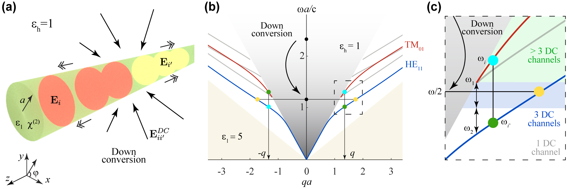
Generation of waveguided entangled photon pairs by down-conversion in an optical waveguide.
(a) Illustration of a cylindrical waveguide (radius a, material permittivity ϵ1, and host permittivity ϵh) subject to normal illumination. Each incident photon can be down-converted via the second-order nonlinear response of the waveguide material (susceptibility χ(2)) to produce two waveguided photons within modes i and i′ characterized by electric fields E
i
and E
i
′
, frequencies ω
i
and ω
i
′
, and wave vectors q
i
and q
i
′
satisfying q
i
+ q
i
′
= 0. (b) Dispersion diagram of waveguide modes (normalized frequency ωa/c as a function of normalized wave vector qa) for ϵ1 = 5 and ϵh = 1. The light cones in the waveguide and host materials (white and gray areas, respectively) limit the existence of guided modes. We highlight the two lowest-order modes that possess nonzero longitudinal field components (HE11 and TM01, see labels) and enable down-conversion with a small number of photon-pair emission channels: one symmetric (yellow circles) and two asymmetric (blue and green circles) channels. (c) Detail of photon-pair emission channels, showing the threshold frequency of the TM01 mode ω1, the frequency ω2 of the HE11 mode with the same wave vector, and the number of down-conversion channels available depending on the incident photon frequency ω (1, 3, and
Without entering into the details of how to quantify entanglement for more complex states [36], we aim at producing maximally entangled photon pairs moving in opposite directions along the waveguide (left L with wave vector −q, and right R with wave vector q) that correspond to Bell quantum states of the form
where i and i′ denote different photon quantum numbers, such as the azimuthal number m, the mode polarization, and the frequency. Before exploring these possibilities, we provide a rigorous theory to calculate the SPDC efficiency associated with different output channels in the waveguide.
2.1 Down-conversion efficiency in cylindrical waveguides
To quantify the SPDC efficiency, we compute the probability of the inverse process: SF generation produced by two counter-propagating guided photons of frequencies ω i and ω i ′ which combine to generate a photon frequency ω ii ′ = ω i + ω i ′ that is normally emitted from the waveguide. In virtue of reciprocity, the per-photon probabilities for the two processes (SPDC and SF generation) are identical. In practice, we calculate the efficiency by considering two photons within counter-propagating guided modes i and i′, prepared as long pulses of length L and space/time-dependent electric fields E i (r, t) and E i ′ (r, t) (Figure 1(a)) that comprise frequency components that are tightly packed around ω i and ω i ′ . Through the SF second-order susceptibility tensor χ(2), a polarization density P ii ′ (R) is produced within a narrow frequency range around ω ii ′ . More precisely,
where the indices {a, b, c} run over Cartesian components, E i (R) gives the profile of mode i in the transverse plane R = (x, y), and we normalize the susceptibility to the quantity
For simplicity, we consider the wave vectors of the two modes to satisfy the condition q
i
+ q
i
′
= 0, so that the SF photons are emitted with zero wave vector component parallel to the waveguide (i.e., along normal directions). The SF polarization density generates a field that we compute at long distances from the waveguide using the electromagnetic Green tensor of the system
After a lengthy calculation (see a detailed self-contained derivation in Methods), we obtain the following result for the angle-resolved efficiency:
where w
i
= ω
i
a/c, β
i
= v
i
/c, v
i
= ∂ω
i
/∂q
i
is the group velocity in mode i, H is the magnetic field, and g(φ − φ′, R′, ω) is the amplitude of the electromagnetic Green tensor in the far-field limit defined through
For the cylindrical waveguides under consideration, we can multiplex the mode labels as i = {q
i
, m
i
, l
i
, σ
i
}, where q
i
is the wave vector, m
i
is the azimuthal angular momentum number, l
i
refers to different radial resonances, and σ
i
runs over polarization states (i.e.,
2.2 Availability and efficiency of different down-conversion channels
We are now equipped to discuss the generation of entangled photon pairs through SPDC in our waveguide. Assuming the above conditions, the lowest-frequency modes that possess a nonzero z component of the electric field, and can consequently couple to normally impinging external light, are HE11 and TM01 (see Figure 1(b)). We identify two relevant frequencies in this region (see Figure 1(c)): the threshold of the TM01 mode at ω1 (satisfying
Another interesting range of incidence frequencies is ω1 + ω2 < ω < 2ω1 (blue area in Figure 1(c)), where the HE11 + HE11 channel is now supplemented by two additional possibilities in which the two generated photons have different frequencies (with the sum satisfying ω = ω i + ω i ′ ) and lie in different bands (HE11 or TM01). This is indicated by the two pairs of color-matched blue and green dots in Figure 1(b) and (c), where the condition of opposite wave vectors is obviously satisfied. Again, it is possible to select a specific SPDC channel by illuminating with a fixed m number (see below), and in particular, by setting m = m i + m i ′ = 1, the HE11 + HE11 channel is eliminated (because the overall azimuthal number obtained by combining two HE±11 modes is 0 or ±2), so that we obtain again a maximally entangled state of the form given in Eq. (1) with i and i′ now referring to TM01 and HE11 (i.e., |LTMRHE⟩ + |LHERTM⟩, with azimuthal numbers m i and m i ′ taking the values 0 and 1 in the TM and HE components, respectively).
The formalism presented in Section 2.1 allows us to calculate the SPDC efficiency for the production of specific photon pair-states, using external illumination prepared with an azimuthal number m = m
i
+ m
i
′
and a polarization state determined by the time reversal of the SF generation state considered in the derivation of these results. Under the assumed conditions of incidence along transverse directions, and considering a zzz-dominant component in the second-order susceptibility tensor, the profile of the applied light amplitude as a function of azimuthal angle φ is therefore taken to be eimφ, with the field oriented parallel to the waveguide direction. These conditions can be met by combining several incident light beams, as we discuss below. The efficiencies calculated for different SPDC channels in this scheme are shown in Figure 2, normalized to
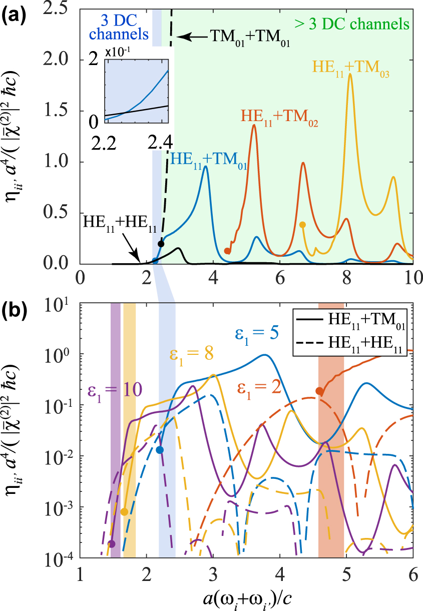
Down-conversion efficiency for different output channels. (a) Normalized SPDC efficiency for a waveguide with ϵ1 = 5 and ϵh = 1 as a function of incident light frequency ω = ω
i
+ ω
i
′
. Different output channels i + i′ are indicated by labels, while the regions highlighted in white, blue, and green indicate 1, 3, and
The spectral evolution of the efficiencies is roughly maintained when varying the waveguide permittivity ϵ1 (Figure 2(b)), but we observe a general increase in η ii ′ with increasing ϵ1 in the region of interest, as well as a spectral shift of the region with three output channels (highlighted in shading colors and evolving toward lower frequencies as we increase the permittivity, in agreement with the single-mode-fiber cutoff condition). Interestingly, we find a crossover in the efficiency of HE11 + HE11 relative to that of HE11 + TM01: the former dominates over the latter within the three-channel region at high ϵ1, whereas the opposite behavior is found at lower permittivities.
Quantitatively, our results indicate that the current scheme is feasible for producing a reasonable rate of entangled photon pairs, taking into account that they are already prepared within waveguide modes [31, 33]. In particular, for values of
2.3 Selection of down-conversion channels through illumination interference
A p-polarized electromagnetic plane wave of amplitude E0 incident through the host medium with a wave vector
in terms of cylindrical waves
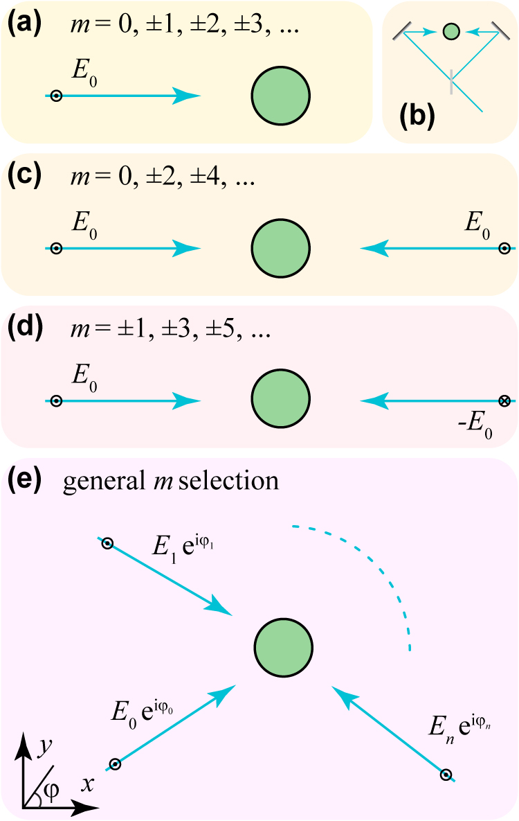
Mode selection through light interference. A single incident light plane wave (a) contains all possible values of the azimuthal number m in the external field, and can thus excite all available SPDC channels for the chosen input frequency. We can combine illumination from different directions through beam splitters and mirrors, as indicated in (b) for two-plane-wave irradiation, leading to a selection of the m values from the external light. Examples of selection by irradiation with two in-phase and out-of-phase counter-propagating plane waves are shown in (c) and (d). More stringent selection of m is possible by combining multiple plane waves of amplitudes E j along different azimuthal directions φ j , with j = 0, …, n.
In the one-channel regime (HE11 + HE11 output), we can generate the maximally entangled state |L−1R1⟩ + |L1R−1⟩ by selecting an incident m = 0 component and eliminating m = ±2 contributions, as other values of m do not couple to the output modes that are available in that region. This selection requires a minimum of three external plane waves (e.g., with equal amplitudes and azimuthal angles of 0 and ±π/3). Likewise, a more stringent selection of m contributions is possible by resorting to more incident plane waves, therefore opening a vast range of possible entangled photon pairs prepared in higher-order modes. In particular, a simple discrete-transform analysis leads to the conclusion that we can select a specific m = m0 component while canceling out those of all other m’s in the |m| ≤ N range by combining 2N + 1 incident waves along azimuthal directions φ
j
= 2πj/(2N + 1) with amplitudes
3 Concluding remarks
We propose a straightforward approach to generate entangled photon pairs directly into low-loss dielectric waveguides based on down-conversion of normally impinging light and introduce a theoretical formalism relying on the reciprocity theorem to quantify the efficiency of the process. Our formalism leads to a universal overall scaling of the efficiency η with the second-order nonlinear susceptibility χ(2) and waveguide radius a as
4 Methods
In this section, we provide a detailed, self-contained derivation of the formalism and equations used in the main text. More precisely, we provide the following elements: a description of guided modes in a cylindrical dielectric wire, along with explicit expressions for their associated electromagnetic fields; a discussion of waveguided pulses; a study of the field produced by line dipoles situated inside the waveguide; a calculation of the SF energy that is emitted into the far field through the second-order nonlinearity of the waveguide material in response to two counter-propagating guided pulses; and a derivation of the SF conversion efficiency, which we argue to be equal to the SPDC efficiency in virtue of reciprocity. We consider guided modes with opposite wave vectors (Figure 1(a)), which couple to external light propagating along directions perpendicular to the waveguide.
4.1 Electromagnetic waves in a cylindrical waveguide
To describe electromagnetic waves in a cylindrical geometry, we first decompose the electric field into cylindrical waves following the prescription of Ref. [40]. More specifically, adopting a cylindrical coordinate system r = (R, φ, z), we consider a homogeneous, isotropic dielectric medium (labeled j) free of external charges and currents that is characterized by a permittivity ϵ
j
(setting the magnetic permeability to μ = 1) and express the electric field in cylindrical waves indexed by their azimuthal number m, wave vector q along
where we define
We now discuss a cylindrical wave emanating from the interior of a cylindrical waveguide of radius a that is infinitely extended in the z direction, comprised of a dielectric material of permittivity ϵ1 (medium j = 1), and embedded in a host medium j = h (permittivity ϵh). Using the notation introduced above, the electric field is expressed as
where
are outgoing waves similar to the propagating waves in Eq. (7), but with the Bessel functions J
m
substituted by Hankel functions
with the matrix M defined as [40]
with k = ω/c. The above result is equivalent to other textbook forms of the dispersion relation for cylindrical waveguide modes [41–44], typically expressed in terms of modified Bessel functions in lieu of Hankel functions. The range of wavelengths λ for which only a single mode exists is determined by the condition
4.1.1 Electric field distribution of guided modes
For convenience, we introduce normalized s- and p-polarized fields defined as
respectively, such that
TE and TM modes – For m = 0 we see from the secular matrix M in Eq. (12) that s and p components are not mixed by scattering at the circular waveguide surface, and therefore, pure-polarization solutions exist in this case, signaled by the vanishing of one of the two factors in the left-hand side of Eq. (13): TE0l modes (s waves) of electric field
HE and HE hybrid modes – For m ≠ 0, the solutions to Eq. (13) are modes of hybrid polarization, EH
ml
and HE
ml
, for which both s and p waves contribute, such that the field of mode i can be expressed as
is defined by imposing continuity of the tangential fields at R = a. When iν > 0 is far from the cutoff frequency, the modes are termed HE ml , while in the opposite situation they are labeled as EH ml . Note that alternative yet equivalent definitions exist depending on how modes are normalized [46].
4.1.2 Waveguided pulses
We consider the propagation of Gaussian wavepackets in the cylindrical waveguide, characterized by a finite spatial pulse width L along the waveguide direction
where E
i
(R, q) is the profile of mode i for a wave vector q. In the pulse, q is tightly packed around q = q
i
. Linearizing the dispersion according to ω ≈ ω
i
+ v
i
(q − q
i
), where
which, after evaluating the integral in q, reduces to
The corresponding magnetic field is readily computed from Faraday’s law H
i
= −(i/k)∇ × E
i
by approximating the ∂
z
component of
with
4.2 Field produced by an inner line dipole in the region outside the waveguide
We consider a line dipole placed at a transverse position R0 = (x0, y0) within the waveguide and represent it by a dipole density
where ∇ is understood to act on r, whereas the integral can be evaluated using the identity
Now, projecting the dipole as
where the fields
4.2.1 Normal emission into the far field
The transmission of electromagnetic fields from the waveguide is determined from Eqs. (9) and (11), which show that, for the special case of q = 0 considered here, polarization states do not mix (i.e., tm,σσ′= 0 for σ ≠ σ′). We thus express the field outside the waveguide produced by a line dipole p placed at R0 as
which is obviously independent of z. In the far field, we can use the asymptotic limit
while the magnetic far field is obtained by using Eq. (8) and Faraday’s law as
where
and the dipole components are defined in Eq. (19).
The above relations allow us to obtain explicit expressions for the far-field limit (khR ≫ 1) of the two-dimensional electromagnetic Green tensor
4.3 Sum-frequency generation by counter-propagating waveguided pulses
We now introduce counter-propagating pulse fields E
i
(r, t) and E
i
′
(r, t) of the form given in Eq. (15), oscillating at frequencies ω
i
and ω
i
′
, respectively. Through the second-order nonlinearity of the waveguide material
where
by defining
Eventually, we set q
i
= −q
i
′
(i.e., waveguided photons with opposite wave vectors, leading to normal emission of SF photons), so v
i
and v
i
′
also have opposite signs inherited from q
i
and q
i
′
. In addition, the nonlinear susceptibility
The SF field E i i ′ (r, t) is thus produced by the nonlinear polarization density according to
where we have introduced the three-dimensional electromagnetic Green tensor
which allows us to recast Eq. (26) as
in terms of the frequency-space electric far-field amplitude
Finally, as shown in Supplementary Information, we can relate the far-field three-dimensional amplitude obtained from the Green tensor in Eqs. (27) and (29) to the two-dimensional one presented in Section (4.2.1) as
with j taking the values +, −, and z. Again, explicit expressions for the components of
4.4 Up- and down-conversion efficiency
The efficiency of the SPDC process in which a photon impinging normally to the waveguide direction produces a pair of guided photons moving in opposite directions away from one another is argued to be identical with that of an up-conversion process involving SF generation of two guided photons moving toward one another, provided that reciprocity applies. We then calculate the SF efficiency η ii ′ = N ii ′ /N i N i ′ as the ratio of the number of emitted SF photons Nii′ to the number of incident photons N i and Ni′ in both guided pulses.
The number of photons carried by a guided mode pulse with field profile E i (r, t) is expressed as
where we evaluate the flux carried by the Poynting vector S i (r, t) = (c/4π)E i (r, t) ×H i (r, t) in the R plane. Inserting the fields given by Eqs. (15) and (16) and integrating over time, we obtain
Likewise, the number of photons produced in the far field via SF generation from the radial component of the energy emanating from the waveguide can be in turn obtained from the far-field Poynting vector
In the derivation of the above expression, we have used the fact that
where
with
with
where the direction
Finally, we specialize the above expressions to q
i
+ q
i
′
= 0 (normal emission, for which
on the difference of the azimuthal angles of
-
Author contribution: All the authors have accepted responsivity for the entire content of this manuscript and approved.
-
Research funding: This work has been supported in part by ERC (Advanced Grant 789 104-eNANO), the Spanish MICINN (PID2020-112625GB-I00 and SEV2015-0522), the Catalan CERCA Program, the Generalitat de Catalunya, the European Social Fund (L’FSE inverteix en el teu futur)-FEDER. J. D. C. is a Sapere Aude research leader supported by Independent Research Fund Denmark (grant no. 0165-00051B). The Center for Nano Optics is financially supported by the University of Southern Denmark (SDU 2020 funding).
-
Conflict of interest statement: The author declares no conflicts of interest regarding this article.
References
[1] S.-B. Zheng and G.-C. Guo, “Efficient scheme for two-atom entanglement and quantum information processing in cavity QED,” Phys. Rev. Lett., vol. 85, p. 2392, 2000. https://doi.org/10.1103/physrevlett.85.2392.Search in Google Scholar
[2] J. M. Raimond, M. Brune, and S. Haroche, “Manipulating quantum entanglement with atoms and photons in a cavity,” Rev. Mod. Phys., vol. 73, p. 565, 2001. https://doi.org/10.1103/revmodphys.73.565.Search in Google Scholar
[3] A. Lamas-Linares, J. C. Howell, and D. Bouwmeester, “Stimulated emission of polarization-entangled photons,” Nature, vol. 412, p. 887, 2001. https://doi.org/10.1038/35091014.Search in Google Scholar PubMed
[4] C. Monroe, “Quantum information processing with atoms and photons,” Nature, vol. 416, p. 238, 2002. https://doi.org/10.1038/416238a.Search in Google Scholar PubMed
[5] T. Inagaki, N. Matsuda, O. Tadanaga, M. Asobe, and H. Takesue, “Entanglement distribution over 300 km of fiber,” Opt. Express, vol. 21, p. 23241, 2013. https://doi.org/10.1364/oe.21.023241.Search in Google Scholar PubMed
[6] S.-K. Liao, W.-Q. Cai, W.-Y. Liu, et al.., “Satellite-to-ground quantum key distribution,” Nature, vol. 549, p. 43, 2017. https://doi.org/10.1038/nature23655.Search in Google Scholar PubMed
[7] D. E. Chang, V. Vuletić, and M. D. Lukin, “Quantum nonlinear optics - photon by photon,” Nat. Photon., vol. 8, p. 685, 2014. https://doi.org/10.1038/nphoton.2014.192.Search in Google Scholar
[8] X. Li, P. L Voss, J. E. Sharping, and P. Kumar, “Optical-fiber source of polarization-Entangled photons in the 1550 nm telecom band,” Phys. Rev. Lett., vol. 94, 2005, Art no. 053601. https://doi.org/10.1103/physrevlett.94.053601.Search in Google Scholar PubMed
[9] J. Liu, I. Nape, Q. Wang, A. Vallés, J. Wang, and A. Forbes, “Multidimensional entanglement transport through single-mode fiber,” Sci. Adv., vol. 6, 2020, Art no. eaay0837. https://doi.org/10.1126/sciadv.aay0837.Search in Google Scholar PubMed PubMed Central
[10] A. Mair, A. Vaziri, G. Weihs, and A. Zeilinger, “Entanglement of the orbital angular momentum states of photons,” Nature, vol. 412, p. 313, 2001. https://doi.org/10.1038/35085529.Search in Google Scholar PubMed
[11] R. Fickler, R. Lapkiewicz, W. N. Plick, et al.., “Quantum entanglement of high angular momenta,” Science, vol. 338, p. 640, 2012. https://doi.org/10.1126/science.1227193.Search in Google Scholar PubMed
[12] M. Malik, M. Erhard, M. Huber, M. Krenn, R. Fickler, and A. Zeilinger, “Multi-photon entanglement in high dimensions,” Nat. Photon., vol. 10, p. 248, 2016. https://doi.org/10.1038/nphoton.2016.12.Search in Google Scholar
[13] T. Stav, A. Faerman, E. Maguid, et al.., “Quantum entanglement of the spin and orbital angular momentum of photons using metamaterials,” Science, vol. 361, p. 1101, 2018. https://doi.org/10.1126/science.aat9042.Search in Google Scholar PubMed
[14] A. S. Solntsev, G. S. Agarwal, and Y. S. Kivshar, “Metasurfaces for quantum photonics,” Nat. Photon., vol. 15, p. 327, 2021. https://doi.org/10.1038/s41566-021-00793-z.Search in Google Scholar
[15] P. G. Kwiat, K. Mattle, H. Weinfurter, A. Zeilinger, A. V. Sergienko, and Y. Shih, “New high-intensity source of polarization-entangled photon pairs,” Phys. Rev. Lett., vol. 75, p. 4337, 1995. https://doi.org/10.1103/physrevlett.75.4337.Search in Google Scholar PubMed
[16] H. H. Arnaut and G. A. Barbosa, “Orbital and intrinsic angular momentum of single photons and entangled pairs of photons generated by parametric down-conversion,” Phys. Rev. Lett., vol. 85, p. 286, 2000. https://doi.org/10.1103/physrevlett.85.286.Search in Google Scholar PubMed
[17] R. W. Boyd, Nonlinear Optics, 3rd ed. Amsterdam, Academic, 2008.Search in Google Scholar
[18] L. G. Helt and M. J. Steel, “Effect of scattering loss on connections between classical and quantum processes in second-order nonlinear waveguides,” Opt. Lett., vol. 40, p. 1460, 2015. https://doi.org/10.1364/ol.40.001460.Search in Google Scholar
[19] R. van der Meer, J. J. Renema, B. Brecht, C. Silberhorn, and P. W. Pinkse, “Optimizing spontaneous parametric down-conversion sources for boson sampling,” Phys. Rev. A, vol. 101, 2020, Art no. 063821. https://doi.org/10.1103/physreva.101.063821.Search in Google Scholar
[20] Z. Yang, M. Liscidini, and J. E. Sipe, “Spontaneous parametric down-conversion in waveguides: a backward Heisenberg picture approach,” Phys. Rev. A, vol. 77, 2008, Art no. 033808. https://doi.org/10.1103/physreva.77.033808.Search in Google Scholar
[21] L. G. Helt, M. J. Steel, and J. E. Sipe, “Spontaneous parametric downconversion in waveguides: what’s loss got to do with it?,” New J. Phys., vol. 17, 2015, Art no. 013055. https://doi.org/10.1088/1367-2630/17/1/013055.Search in Google Scholar
[22] F. Lenzini, A. N. Poddubny, J. Titchener, et al.., “Direct characterization of a nonlinear photonic circuit’s wave function with laser light,” Light Sci. Appl., vol. 7, p. 17143, 2018. https://doi.org/10.1038/lsa.2017.143.Search in Google Scholar PubMed PubMed Central
[23] E. Pomarico, B. Sanguinetti, N. Gisin, et al.., “Waveguide-based OPO source of entangled photon pairs,” New J. Phys., vol. 11, p. 113042, 2009. https://doi.org/10.1088/1367-2630/11/11/113042.Search in Google Scholar
[24] K.-H. Luo, H. Herrmann, S. Krapick, et al.., “Direct generation of genuine single-longitudinal-mode narrowband photon pairs,” New J. Phys., vol. 17, 2015, Art no. 073039. https://doi.org/10.1088/1367-2630/17/7/073039.Search in Google Scholar
[25] V. S. Ilchenko, A. A. Savchenkov, A. B. Matsko, and L. Maleki, “Nonlinear optics and crystalline whispering gallery mode cavities,” Phys. Rev. Lett., vol. 92, 2004, Art no. 043903. https://doi.org/10.1103/physrevlett.92.043903.Search in Google Scholar PubMed
[26] X. Guo, C.-l. Zou, C. Schuck, H. Jung, R. Cheng, and H. X. Tang, “Parametric down-conversion photon-pair source on a nanophotonic chip,” Light Sci. Appl., vol. 6, 2017, Art no. e16249. https://doi.org/10.1038/lsa.2016.249.Search in Google Scholar PubMed PubMed Central
[27] J. W. Silverstone, D. Bonneau, K. Ohira, et al.., “On-chip quantum interference between silicon photon-pair sources,” Nat. Photon., vol. 8, p. 104, 2014. https://doi.org/10.1038/nphoton.2013.339.Search in Google Scholar
[28] F. Setzpfandt, A. S. Solntsev, J. Titchener, et al.., “Tunable generation of entangled photons in a nonlinear directional coupler,” Laser Photon. Rev., vol. 10, p. 131, 2016. https://doi.org/10.1002/lpor.201500216.Search in Google Scholar
[29] Z. Sun, D. Basov, and M. Fogler, “Graphene as a source of entangled plasmons,” arXiv preprint arXiv:2110.14917, 2021.10.1103/PhysRevResearch.4.023208Search in Google Scholar
[30] L. Novotny and B. Hecht, Principles of Nano-Optics, Cambridge, Cambridge University Press, 2006.10.1017/CBO9780511813535Search in Google Scholar
[31] A. De Rossi and V. Berger, “Counterpropagating twin photons by parametric fluorescence,” Phys. Rev. Lett., vol. 88, 2002, Art no. 043901. https://doi.org/10.1103/physrevlett.88.043901.Search in Google Scholar
[32] M. C. Booth, M. Atatüre, G. Di Giuseppe, B. E. Saleh, A. V. Sergienko, and M. C. Teich, “Counterpropagating entangled photons from a waveguide with periodic nonlinearity,” Phys. Rev. A, vol. 66, 2002, Art no. 023815. https://doi.org/10.1103/physreva.66.023815.Search in Google Scholar
[33] A. Orieux, X. Caillet, A. Lemaître, P. Filloux, I. Favero, G. Leo, and S. Ducci, “Efficient parametric generation of counterpropagating two-photon states,” J. Opt. Soc. Am. B, vol. 28, p. 45, 2011. https://doi.org/10.1364/josab.28.000045.Search in Google Scholar
[34] A. Orieux, A. Eckstein, A. Lemaître, et al.., “Direct Bell states generation on a III-V semiconductor chip at room temperature,” Phys. Rev. Lett., vol. 110, p. 160502, 2013. https://doi.org/10.1103/physrevlett.110.160502.Search in Google Scholar PubMed
[35] S. Saravi, T. Pertsch, and F. Setzpfandt, “Generation of counterpropagating path-entangled photon pairs in a single periodic waveguide,” Phys. Rev. Lett., vol. 118, p. 183603, 2017. https://doi.org/10.1103/physrevlett.118.183603.Search in Google Scholar
[36] M. B. Plenio and S. S. Virmani, An Introduction to Entanglement Theory, Cham, Springer International Publishing, 2014, pp. 173–209.10.1007/978-3-319-04063-9_8Search in Google Scholar
[37] H. Jin, F. M. Liu, P. Xu, et al.., “On-chip generation and manipulation of entangled photons based on reconfigurable lithium-niobate waveguide circuits,” Phys. Rev. Lett., vol. 113, p. 103601, 2014. https://doi.org/10.1103/physrevlett.113.103601.Search in Google Scholar
[38] Y. Kong, F. Bo, W. Wang, D. Zheng, H. Liu, G. Zhang, R. Rupp, and J. Xu, “Recent progress in lithium niobate: optical damage, defect simulation, and on‐chip devices,” Adv. Mater., vol. 32, p. 1806452, 2020. https://doi.org/10.1002/adma.201806452.Search in Google Scholar PubMed
[39] V. G. Dmitriev, G. G. Gurzadyan, and D. N. Nikogosyan, Handbook of Nonlinear Optical Crystals, vol. 64, 3rd ed. Berlin, Springer, 1999.10.1007/978-3-540-46793-9Search in Google Scholar
[40] F. J. García de Abajo, A. Rivacoba, N. Zabala, and P. M. Echenique, “Electron energy loss spectroscopy as a probe of two-dimensional photonic crystals,” Phys. Rev. B, vol. 68, p. 205105, 2003. https://doi.org/10.1103/physrevb.68.205105.Search in Google Scholar
[41] G. P. Agrawal, Nonlinear Science at the Dawn of the 21st Century, Berlin, Springer, 2000.Search in Google Scholar
[42] G. Keiser, Optical Fiber Communications, New York, McGraw-Hill, 2011.Search in Google Scholar
[43] D. Marcuse, Theory of Dielectric Optical Waveguides, 2nd ed. San Diego, Academic Press, 2013.Search in Google Scholar
[44] R. Engelbrecht, Nichtlineare Faseroptik: Grundlagen Und Anwendungsbeispiele, Berlin, Springer-Verlag, 2015.10.1007/978-3-642-40968-4Search in Google Scholar
[45] B. E. Saleh and M. C. Teich, Fundamentals of Photonics, New York, John Wiley & Sons, 2019.Search in Google Scholar
[46] C. Yeh and F. I. Shimabukuro, The Essence of Dielectric Waveguides, Berlin, Springer, 2008.10.1007/978-0-387-49799-0Search in Google Scholar
[47] M. Abramowitz and I. A. Stegun, Handbook of Mathematical Functions, New York, Dover, 1972.Search in Google Scholar
[48] DLMF, NIST Digital Library of Mathematical Functions, Release 1.1.3 of 2021-09-15, f. W. J Olver, A. B. Olde Daalhuis, D. W. Lozier, et al.., Eds. Available at: http://dlmf.nist.gov/.Search in Google Scholar
Supplementary Material
The online version of this article offers supplementary material (https://doi.org/10.1515/nanoph-2021-0736).
© 2022 Álvaro Rodríguez Echarri et al., published by De Gruyter, Berlin/Boston
This work is licensed under the Creative Commons Attribution 4.0 International License.
Articles in the same Issue
- Frontmatter
- Reviews
- Photonic neuromorphic technologies in optical communications
- Photo-modulated optical and electrical properties of graphene
- Optical metasurfaces for generating and manipulating optical vortex beams
- Research Articles
- Photon coupling-induced spectrum envelope modulation in the coupled resonators from Vernier effect to harmonic Vernier effect
- Generation of high-uniformity and high-resolution Bessel beam arrays through all-dielectric metasurfaces
- Controlling and probing heat generation in an optical heater system
- Nonthermal laser ablation of high-efficiency semitransparent and aesthetic perovskite solar cells
- Plasmon-enhanced photoluminescence from MoS2 monolayer with topological insulator nanoparticle
- Polarization-controlled anisotropy in hybrid plasmonic nanoparticles
- Empirical formulation of broadband complex refractive index spectra of single-chirality carbon nanotube assembly
- Direct generation of entangled photon pairs in nonlinear optical waveguides
- A high-gain cladded waveguide amplifier on erbium doped thin-film lithium niobate fabricated using photolithography assisted chemo-mechanical etching
- High-performance near-infrared photodetectors based on gate-controlled graphene–germanium Schottky junction with split active junction
- Nonlinear thermal lensing of high repetition rate ultrafast laser light in plasmonic nano-colloids
- Ultra-secure optical encryption based on tightly focused perfect optical vortex beams