Quantifying nucleation in flow by video-FLIM

2.1 Micro fluidic for anti-solvent precipitation

By mixing a solution of a solute in a good solvent with a non-solvent of the solute that is fully miscible with the good solvent, a precipitation by anti-solvent occurs. Supersaturations as high as C/Cs = 1,000 can be achieved allowing the precipitation of both crystalline and amorphous phases.

The challenge of the precipitation in microfluidics is to get the nucleation in the flow rather than on the walls. We use a co-flow geometry where the solute is injected into the centre of the microchannel [11]. The anti-solvent focusing effect, which repels the molecule towards the centre of the flow, limits the precipitation on the walls [6] (Figure 1).

Figure 1:

The microfluidic setup for the observation of antisolvent precipitation. After the injection of a concentrated solution of the solute by the nozzle, a hydrodynamic expansion of the flow is observed over 50 μm “Exp.”. It is followed by an interdiffusion of the solvent and anti-solvent “Dif.”. The solute is repelled and concentrated until it reaches the spinodal concentration “Spin.” a few mm away where the liquid phase appears in a barrierless process [6]. Crystallization of the droplets occurs later. A picture of the microfluidic device is displayed. The two syringe pumps 1 and 2 are used to adjust the flow rate and the composition of the solute solution that flows through the nozzle. A double syringe pump with two syringes (3) and (4) and a 6-port valve (5) are used to flow the anti-solvent in the capillary and replace it by the solvent in order to wash the device as soon as crystals start to grow on the wall. The two other syringe pumps are used to adjust the flow rate and the composition of the solute solution.

The outer capillary is a cylindrical borosilicate tube (CV2033 from Vitrocom, inner diameter 200 μm, outer diameter 330 μm).

The injection nozzle is a quartz capillary tube with an outer diameter of 90 µm. Both are supplied by Molex Polymicro (Lisle, IL 60532, USA).

The tip is forged into a parabolic profile in order to reduce the dead zone and the turbulence at the injection point. This shape is obtained by pulling the capillary with a home-made pipet puller. The optimal tip: straight drawn capillary, large outlet, smooth surface is obtained after one week of self-training by adroit users.

The nozzle is centred in Z when its image is sharp in the middle plan. This position is not favoured by the lamellar flow and is lost when bubbles pass by. We do not have a protocol for the centring. But we can move the injection nozzle inside the capillary through the Upchurch Scientific FEP sleeve of 70–110 µm inner diameter until it is in the correct position.

The assembly of the capillary uses the HPLC technology and the standard 1/16 high-pressure connectors from Upchurch Scientific. Flows are fixed by syringe pump (Fusion 4000, Chemix Inc., Texas, USA) using gas tight glass and Teflon syringe (VWR, Rosny-sous-Bois, France). Crystals appear continuously in the flow within 1 cm of the nozzle, at a rate up to 10 s⁻¹. A 6-port valve is used to replace the anti-solvent with the solvent to rinse the unit as soon as crystals start to grow on the wall. This happens every 10 min. This is long enough to characterise the birth of tens of crystals. Dust and air bubbles must be removed. The saturated solution flow is filtered through a PVDF filter with 0.45 µm pores at the entrance of the nozzle capillary. Bubbles are removed from the syringes and from the dead volumes of connectors before the assembly in order to have well-defined flow rate.

2.2 The solute and solvents

As an anti-solvent we use water the most commonly used precipitating agent. As a solvent for DBDCS, we use 1,4-Dioxane, which is an aprotic, apolar solvent but still miscible with water. The miscibility is total, but at the limit of the separation. In the framework of the regular solution model, the Gibbs energy of mixing ΔG_mix is given by:

where x _i , x _j are the molar fractions of the two solvents. The parameter Ω_{Water,Dioxane} has a value of +4,310 K/mol = 1.74 kT [5]. It is interpreted as excess energy of the intermolecular interaction between the molecules of the two solvents. Its positive value opposes to the miscibility. For 1,4-Dioxane, this enthalpic term is just counter balanced by the entropy of the mixing at room temperature.

The densities are of 0.997 g/mL for water and 1.029 g/mL for 1,4-Dioxane at 20 °C with a slight volume contraction on mixing [12]. This is to avoid sedimentation of the liquids in the microflow.

The refraction index of water and 1,4-Dioxane are respectively 1.3312 and 1.4197 at 632 nm [13]. This is enough to follow the solvent boundaries during the mixing (Figures 2).

Figure 2:

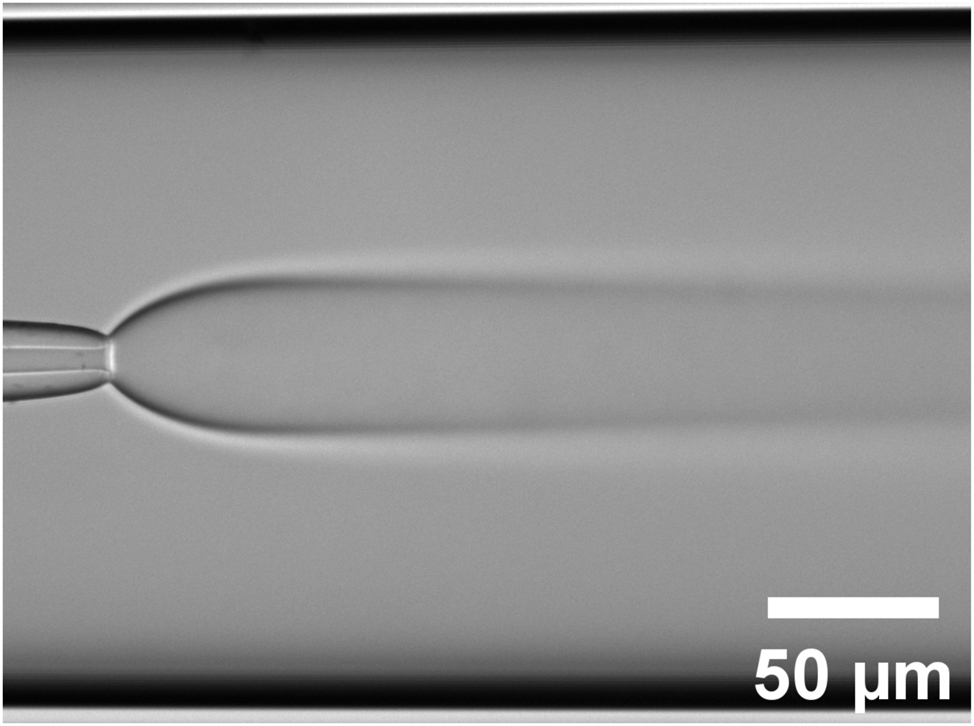
The injection nozzle (5 µm inner diameter) is centered inside the cylindrical capillary (200 µm inner diameter). The 1,4-Dioxane solution is injected at a rate of (400 nL/min) into water (1 μL/min). The initial expension of the inner flow is followed by the interdiffusion of the two solvents. The contrast in this transmission image is due to the gradient of refraction index in the shadowgraph illumination mode.

Figure 3:

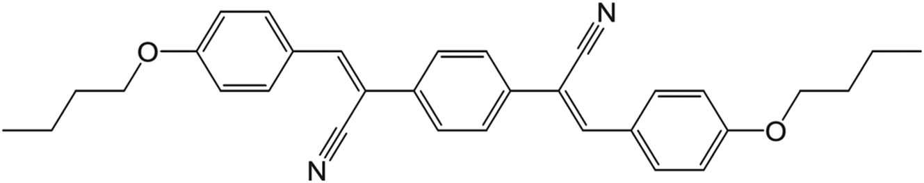
Molecular structure of DBDCS ((2Z,2′Z)-2,2′-(1,4-phenylene)bis(3-(4-butoxyphenyl) acrylonitrile)). Formula: C₃₂H₃₂N₂O₂; molecular mass: 476.60 g/mol.

The solute, DBDCS is displayed in Figure 3.

DBDCS is not fluorescent as a molecule in solution but that becomes fluorescent in the solid state. It exhibits aggregation induced emission: AIE [10]. This allows the detection of fluorescent crystal nucleation and growth against a non-fluorescent background. Two polymorphs of DBDCS have been reported to switch under shear stress: the γ phase (green emission, fluorescence lifetime >10 ns) and the β phase (blue emission, fluorescence lifetime <6 ns) [14].

In the following, one condition of precipitation is studied. It is the injection of a solution of DBDCS at 16 g/L (33 mmol/L) at a flow rate of 400 nL/min into an anti-solvent mixture with a flow rate of 1 μL/min. The anti-solvent is composed of 30 % of 1,4-Dioxane in 70 % of water in volumes.

2.3 Microscopy in a cylindrical tube

We use an epifluorescence microscope. The excitation beam at 343 nm is the third harmonic of an ytterbium tungstate laser (Goji, Amplitude, Pessac, France). Part of the IR beam is used to trigger a fast photodiode with constant fraction discriminator (OCF400, Becker & Hickl GmbH, Berlin, Germany) for the single photon timing. The laser is focused on the back focal point of the objective in order to be collimated at the sample plane. It is expanded to cover the entire field of view with less than 10 % variation in excitation intensity between the centre and the edge.

The microfluidic device in placed in an inverted microscope (TE2000-U, Nikon, Japan). The objective is a CFI S Plan Fluor ELWD objective (Nikon, Japan), WD 8.2–6.9 mm, magnification 20×, NA = 0.45, infinite corrected, correction ring range from 0 to 2.6 mm. It is used with a parfocal length extender ring of 5 mm thickness to achieve the correct traveling distance of the focusing at the sample plane. The cylindrical tube is placed between two coverslips and immersed in water as the index matching liquid. A Retiga R1 CCD camera (Teledyne Photometrics, Tucson, Arizona, USA) runs under μManager [15] (Figure 4).

Figure 4:

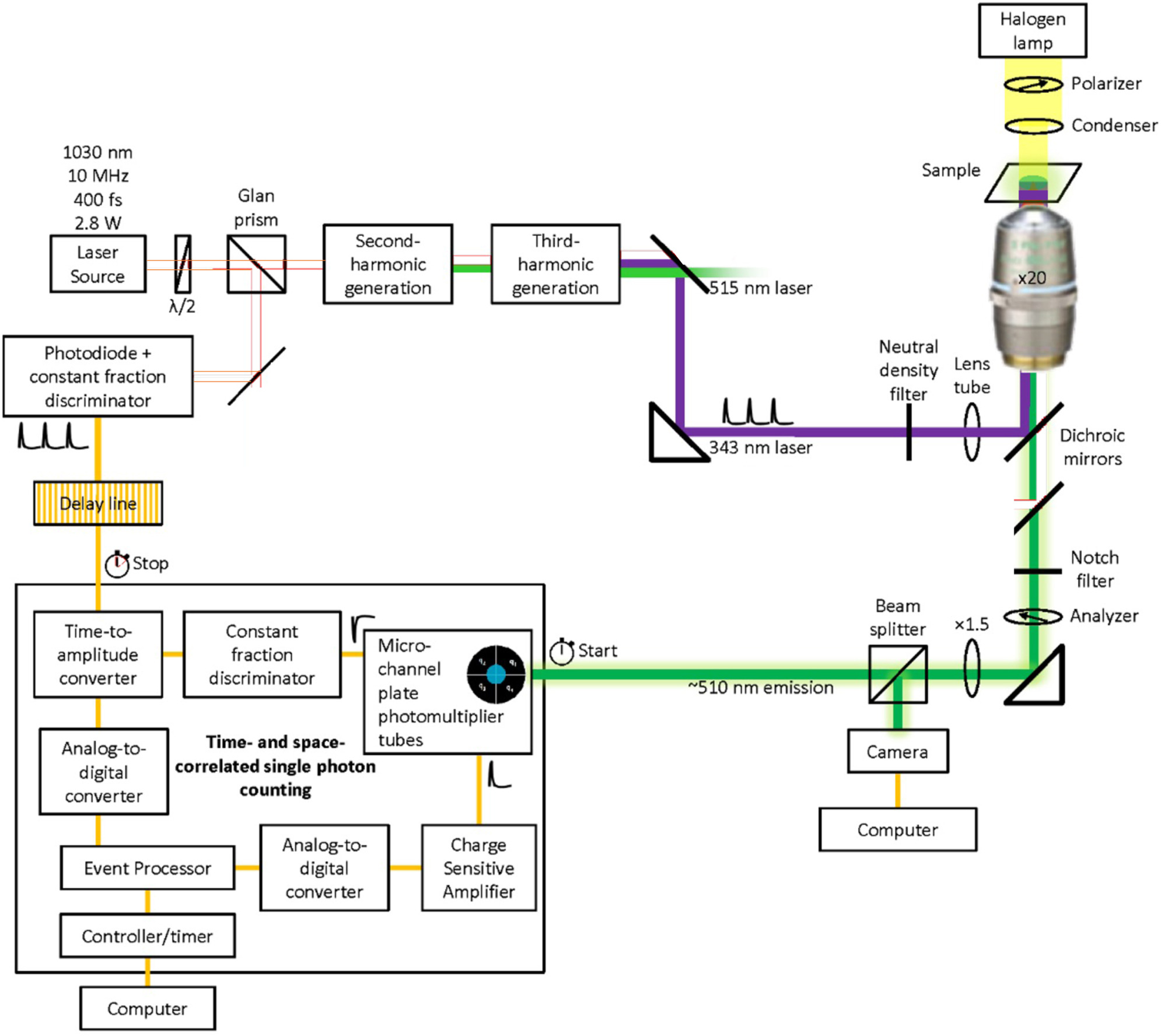
Space and time localised single photon counting. The third harmonic of a pulsed Ytterbium tungstate laser is used to shine uniformly the fluorescent sample. The LINCam time and space resolved single photon counting detector collects and stores all the emitted photons with their fluorescence delay (<100 ns) and absolute arrival time (>100 ns).

2.4 The LINCam

The LINCam (2007 version, Photonscore, Magdeburg, Germany) [16]. LINCam is a localisation PMT that counts the avalanche induced by photons one by one. One photon bumps an electron out of the photocathode. This electron is accelerated and passes through two multichannel plates creating one avalanche of 10⁶ electrons. The centre of the avalanche is precisely correlated in time and space with the initial photon. This avalanche is 1 cm wide and lasts 3 ns when it reaches the anode. Then super-resolution is used to localise the centre of the avalanche in both time and space. The arrival time of the photon can be measured with an accuracy of 60 ps using a constant fraction discriminator. The position of the avalanche is measured using multi-anodes. The position of the centre is calculated as the weighted average of the charge measured by each sub-anode. It can be measured with an accuracy of 24 µm over the 25 mm of the photocathode. This corresponds to camera with 1,024 virtual pixels.

2.5 Images and profiles reconstruction

All calculations were performed using Igor Pro work environment (WaveMetrics Lake Oswego, Oregon, USA).

Each photon is stored with at least 4 data. Its X and Y position on the photocathode, its TAC the time between the arrival of the laser and detection of the photon (fluorescence delay) and its TAbs the time from the start of the recording. The acquisition time depends on the type of data that we want to compare. The data collected to construct a decay occupy 5 Mo of disk space. An intensity image requires 50 Mo whereas a FLIM image occupies 250 Mo. We create 1 or 2 Go files only when particularly interesting conditions have been found. The size of the files is doubled if the HDF5 format [17] is chosen.

Data processing is all about histograms id est projecting these 4D data sets into 1D or 2D representations.

The total fluorescence decay is just the number of photons collected as a function of the fluorescence delay TAC.

Fluorescence bleaching is just the number of photons collected as a function of the acquisition time TAbs. This can be written as:

where dwell is the sampling time in second. δ_i,TAbs is 1 if a photon i was detected between Tabs and Tabs + dwell and 0 otherwise. ∑ i is the sum over all collected photons.

The fluorescence image is simply the number of photons collected as a function of the pixel position X and Y.

where δ_i,X,Y equals 1 if the photon i falls in the pixels [X,X + PixelSize] and [Y,Y + PixelSize] where PixelSize is the size of the virtual pixel chosen for the image. X and Y are coded between 0 and 4,095. We are usually using a 512 × 512 image.

The evolution of the fluorescence lifetime along the recording can be calculated by:

where TAC _i is the fluorescence delay of photon i.

An example of the three signals is represented on Figure 5.

Figure 5:

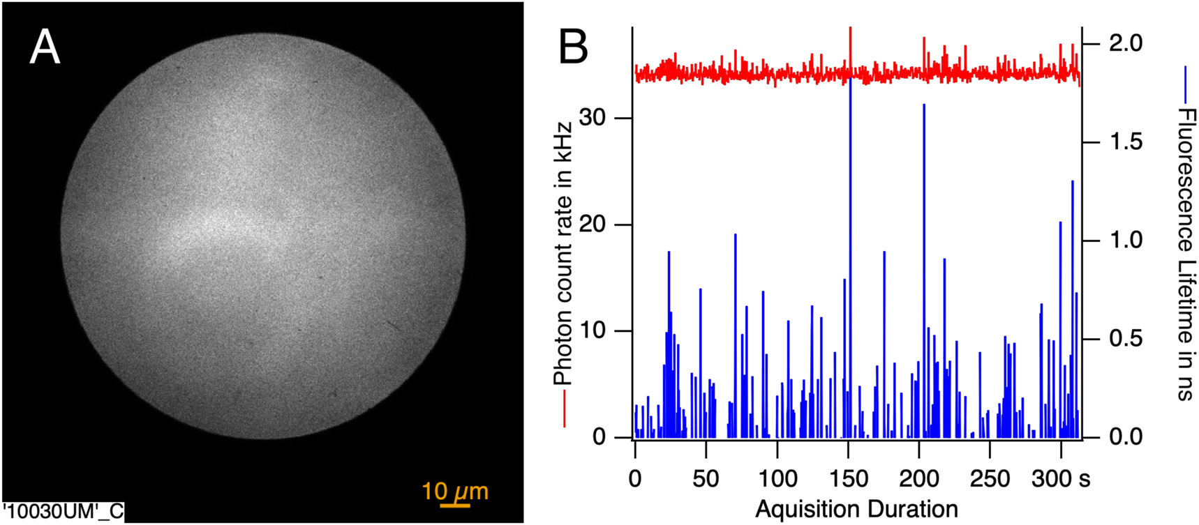
In (A) the fluorescence intensity image in the flow 10.03 mm away from the nozzle integrated over the acquisition time. Molecules and their fluorescence fill the entire observation area. In (B) the instantaneous intensity is shown in red and the instantaneous lifetime is shown in blue. The presence of peaks within both curves reveals the passage of crystals through the field of view.

The fluorescence lifetime image obtained by calculating for each pixel X,Y the ratio:

The FLIM image taken at different positions along the flow are gathered on Figure 6. FLIM shows the formation of a flow of crystals in the centre of the capillary.

Figure 6:

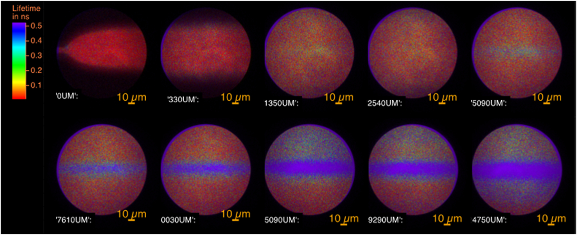
The FLIM images of the flow of fluorescent molecules at different positions from the nozzle expressed in µm. At 0 µm, the hydrodynamic expansion of the concentrated solution of the solute into the antisolvent is seen. The fluorescence of the molecules is characterised by its short lifetime. From 5,090 µm, the crystals appear in the centre of the flow with a long lifetime. In between is the fluorescence of the amorphous phase.

3.1 Reconstruction of the flux

The data are collected from a flow of particles moving at a constant velocity. The flux through a surface normal to the flow at position X varies with time. The intensity time profile through a line at position X is 1 dwell ∑ i δ i , TAbs , X where the collected photons are those detected at position X and at time Tabs. However, we lose the information contained in the photons collected out of this line.

Let us assume that objects move at a constant speed v. Then a photon detected at time Tabs + ∆TAbs and at position X + v∆TAbs contains information from the same object and can be added to the signal. Using these photons, the intensity of the particle flux at X and at time TAbs is given by:

where δ i , TAbs + Δ TAbs , X + v Δ TAbs equals 1 if the photon i detected at TAb s i , X i verifies that

TAbs _i is between [Tabs + ∆Tabs, Tabs + ∆Tabs + dwell] and X _i is between [X + V∆Tabs, X + V∆Tabs + Binning] and zero otherwise.

In the same way:

This treatment is illustrated in Figure 7(A) and (B), which show a sample where individuals crystals can be seen flowing through. In (A), the raw intensity and lifetime profiles obtained by collecting all the photons in the image are shown. The peaks are broad, with a common width equal to the transit time of the crystal through the field of view, 80 ms in this case.

Figure 7:

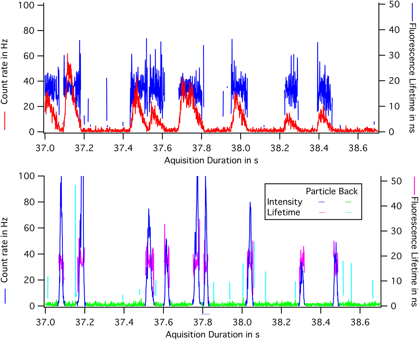
Signal profiles through the window and through a line: (A) The instantaneous intensity and the lifetime of the field of view. Photons collected 500 ps after the laser pulse are selected. They are emitted by the crystals. Bursts are caused by the passage of a particle. The width of the burst is the same for all bursts: 80 ms. It is the duration of the passage of the crystal in the field of view. (B) Intensity and the lifetime corrected for the translation of the flow. By applying a threshold to the intensity curve, it is possible to define the lifetime of a particle, its total intensity and its minimum width.

In (B), the signal from a line at X increased by the photons of the same particle collected later during the translation of the particle is shown. The same number of photons are now gathered in narrow peaks. The two particles that overlapped at time 37.8 s are now separated.

The value of the velocity used to correct for the translation is that of the flow. This velocity is not uniform in a microcapillary and is that given by Poiseuille’s law in the case of cylinders with laminar flows. Fortunately, due to the anti-solvent focusing, which repels the solute molecule towards the centre of the capillary, the maximum nucleation probability is at the centre of the flow [6]. The velocity at the cenyer in twice the average flow rate and can be estimated by [18]:

where R is the radius of the capillary, Q is the flow rate.

The value of the speed v can be further adjusted in order to minimize the peaks width. v = 1.165 mm/s in that experiment.

We successfully formed images of the crystals with the measuring system. To have enough photons we must sum all the images during the transition time of the crystals in the field of view of the system. This sum causes a blurring of the image in the direction of movement of the crystal. As we know the speed v of the forming crystal, we summed the images by shifting to compensate the speed v in order to obtain a more precise image. When we analyse the intensity of the crystals corrected for the speed, we obtain the curve in Figures 7B).

Figure 8:

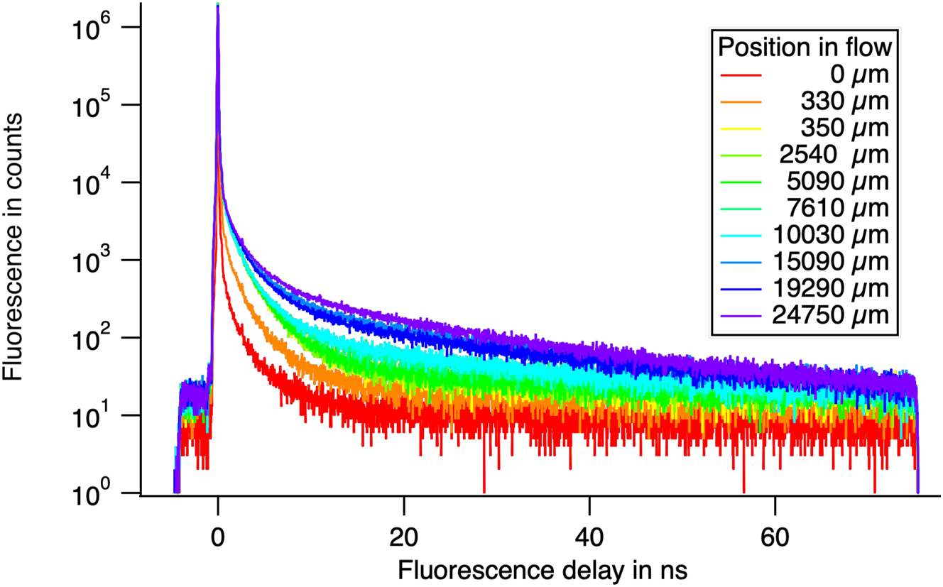
A collection of decays measured at increasing distances from the nozzle at the centre of the flow. At short distances, the short decay is that of the molecules. We see the development of a long-lived decay associated with crystals.

3.2 Counting polymorphs by principal component analysis

The dispersed molecules, the amorphous phase and the different polymorphs of DBDCS have different fluorescence decay signatures [19]. The decay for a given polymorph is not necessarily exponential due to the presence of defects in the crystal [20]. Nevertheless, it possible to calculate the contribution of each reference decay for each pixel following the Principal Component Analysis (PCA) method [21].

Each fluorescence decay collected over 4,096 channels in any part of the image can be considered as a vector in a 4,096-dimensional space Figure 8. Typical decays can be collected from different part of the image, including parts where a pure phase is expected such as the molecules inside the nozzle, different crystals growing on the walls. In our example, N = 16 typical decays were collected. If there are only four species in the image, these N decays should be confined to a 4-dimensional space. To show this, we will try to construct a four members basis describing the data.

Let us first define a scalar product, which is a generalization of the Euclidean scalar product to this 4,096-dimensional space. The scalar product is given by:

The length is given by:

The PCA provides an orthonormal base that exhaustively describes the 16 typical decays. It consists of 16 elements. The first member of the base, the first principal component CP0, was chosen to minimise the total distance between decays and the CP0 direction.

where I _j are the N = 16 typical decays.

After CP0 has been found, the projections of the decays in a subspace orthogonal to CP0 I j − I j ◦ CP 0 CP 0 are computed. CP1, CP2, …, CPN are constructed recursively on these projections.

Suppose that the square of the norm of a decay is an estimate of the information, it contains. Then ∑ j ⊂ 0 , N [ I j ◦ CP 0 2 represents the fraction of this information that is described by the principal component CP0. Figure 9 shows the contribution of all principal components to the description of the information are displayed. For the first four components there is a rapid decrease of this contribution, followed by a plateau. We assume that the components beyond CP3 describe noise.

Figure 9:

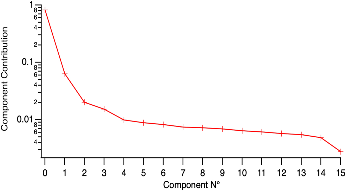
The contributions of the components to the description of the data. We shall assume that CP0 to CP3 are important and that the others describe the noise in the data.

An indication that four components correctly describe our data is obtained by plotting the weighted residuals for this four components model. The residuals of the description of all the fluorescence decays collected in the FLIM map of spontaneous crystallisation by the four principal components are plotted in Figure 10. The sign and the amplitude of the residual is random everywhere except in the range −718 ∼ 504 ps. This time range was removed from the analysis as it mostly describes molecular fluorescence. This means that we have a good description of the data by assuming the presence of four species.

Figure 10:

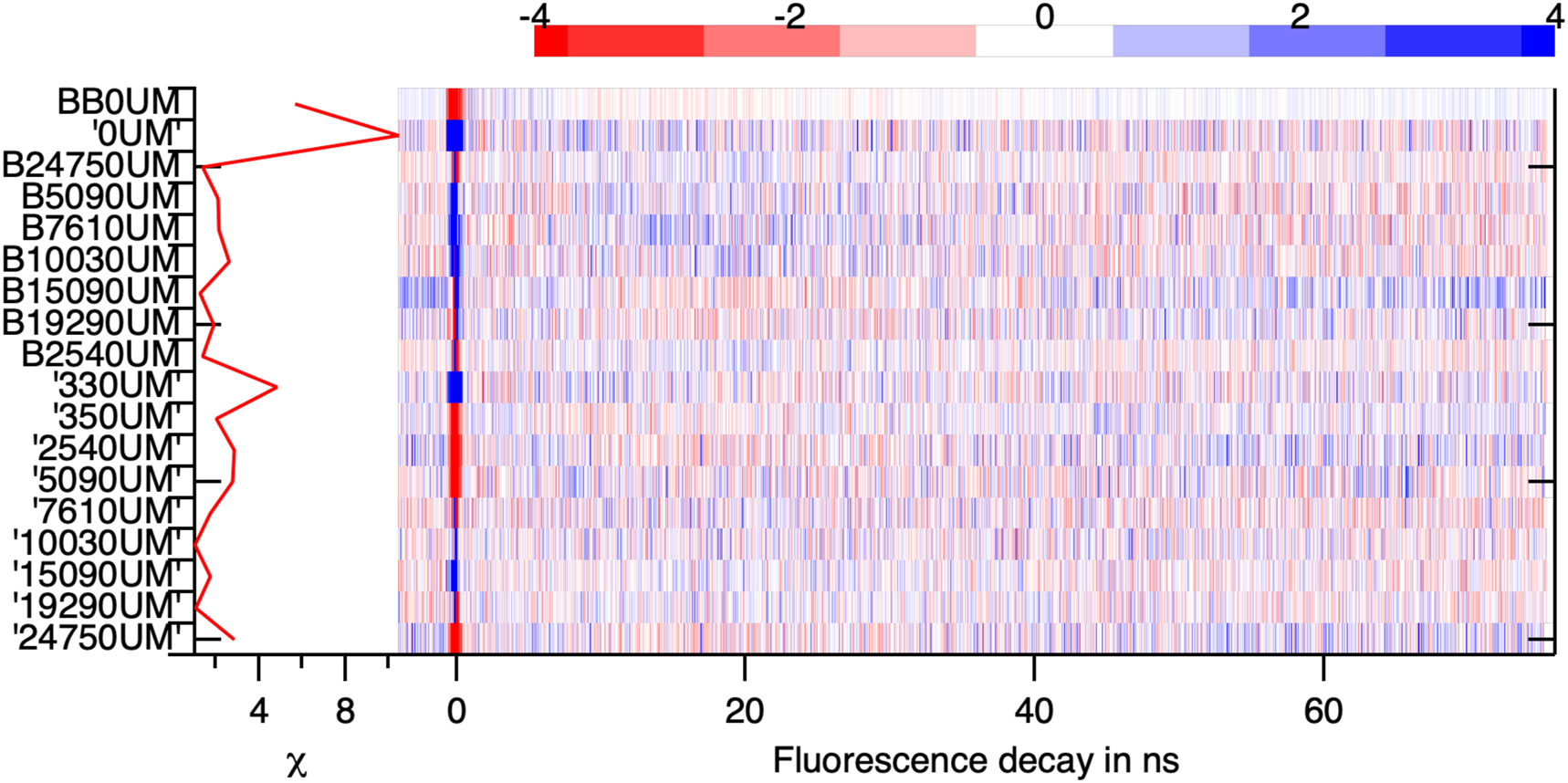
The weighted residuals, the difference between the data and their description by the four components, divided by the expected amplitude of the noise. The random change in sign and the small amplitude of the weighted residuals indicates the quality of the description of the data by the model.

3.2.1 Constructing the signature of the polymorphs

The four principal components do not represent the fluorescence decay of the four species. These decays must be constructed as a linear combination of the principal components, since any linear combination will describe the data as well as the principal components. The constructed decays must obey two constrains, since they are associated with concentrations: they must be positives at any time, and their contribution to the fluorescence of any part of the image should be positive.

Three components can be obtained from locations where only one component might be expected.

1. “Microscope”: the fluorescence of the microscope and room light that was measured in the dark area of the nozzle image.

2. “Molecules”: the fluorescence that was measured in the bright area of the nozzle image.

3. “Amorphous”: the decay that was collected from the flow periphery of the 15,090 µm image where it was supersaturated but without crystals.

   A time constrain is added for the last decay:

4. “CPFluctant” has been chosen to fully describe the fluctuating part of the intensity. It is associated to flowing single objects.

This condition uniquely defines CPFluctuant Figure 11. It appears that CPFluctant presents a long component with a lifetime of 23 ± 2 ns and a short component of 4 ± 2 ns. The 23 ns component is that of the green phase of DBDCS crystals. The 4 ns component is the red phase of DBDCS crystals [14].

Figure 11:

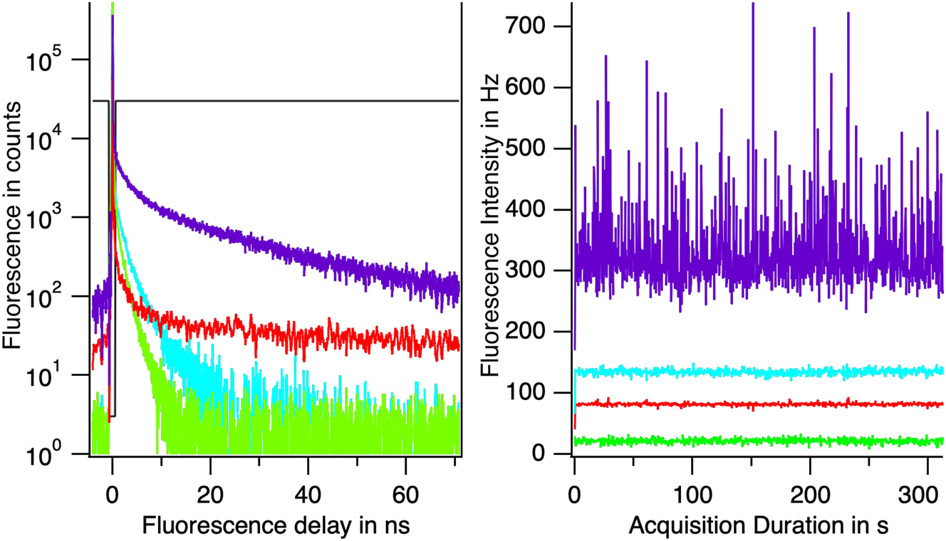
Reconstructed fluorescence of some constituents of the flow: the fluorescence from the microscope and room light is shown in red; molecule fluorescence is shown in green; in cyan, the amorphous phase; in violet the crystals. On the left the fluorescence decays. On the right the fluorescence intensity during the recording.

3.2.2 Polymorphs concentrations

From this attribution, we can check some properties of the system. The contribution of the “Amorphous” DBDCS and the crystals to the fluorescence intensity in the two regions of interest along the microflow are plotted in Figure 12. The contribution of the crystal in the central flow increases along the flow (right plot). Whereas the contribution of “Amorphous” is high and constant in the peripheral flow (left plot).

Figure 12:

Contribution of the amorphous DBDCS (red cross) and the crystals (red hexagon) to the fluorescence intensity in the two regions of interest along the microflow. Left: in the side flow; Right: in the centre of the flow. The contribution of “CPFluctuant” in the centre of the flow increases with the residence time in the device with few crystals in the flow periphery.

3.3 Counting polymorphs by single particle analysis

Molecules produce a fluorescence in the first 500 ps. By selecting late fluorescence photons, we can selectively detect the fluorescence of crystals. If the crystals are large enough, they can be detected one by one (Figure 7).

3.3.1 Nucleation rate

The crystal production rate in our device is the number of crystals produced per second. The number of crystals as a function of the observation time is shown in Figure 13 (left). It gives a nucleation time of 0.713 ± 0.001 s at 7,610 µm from the nozzle. Fewer crystals are counted at shorter distances. This may be because they are too small to be detected or because nucleation still occurs up to 7,610 µm.

Figure 13:

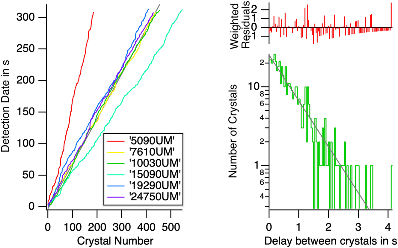
The time interval between the occurrence of nucleation events. Left: the arrival time of individual crystals at different positions along the flow. The slope provides the nucleation time. Except for the position 15,090 µm, there is a conservation of the number of crystals after 7,610 µm. The flux of crystals is conserved. Right: for a nucleation process occurring with a constant probability, we anticipate an exponential distribution of the number of crystals observed as a function of the time between two nucleations. The straight line of the left plot demonstrates the constant production rate of crystals in the device. But a constant production rate does not mean a constant interval between nucleation events as shown in the right plot.

Since the production in the flow is a steady process, the production rate is constant and the probability of detecting a crystal is constant. Nucleation, however, is a random single event. The distribution of the time between two crystals is represented on Figure 13 (right). In accordance with the theory of Poisson point process, the distribution of times between nucleation events is an exponential. The slope of the semi-log plot gives a second estimate of the nucleation time with a value of 0.74 ± 0.03 s [22].

3.3.2 Crystal size

The peak area in Figure 7B represent the total intensity emitted by a crystal as it traverses the field of view of the LINCam. The high absorption cross section of the DBDCS crystals at 353 nm result in an excitation penetration depth of less than 1 µm. The fluorescence intensity of a crystal is proportional to its area. This area can be compared to the length of the crystal as measured by its transit time. Indeed, after correcting for the transit time through the LINCam field of view, a minimal width is observed. This is the time taken by crystals to pass through the reference line used for the flux calculation.

These two methods of estimating crystals size are compared in Figure 14 which plots the fluorescence intensity of individual crystals as a function of their transit time through the reference fictive line. As anticipated, a quadratic dependence is observed, although a deviation from the quadratic law is evident for small crystals.

Figure 14:

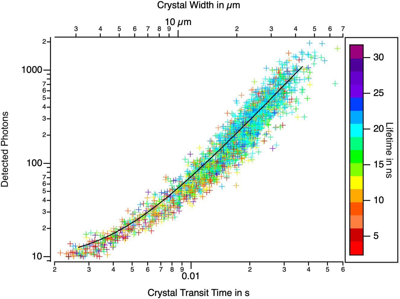
The total number of photons counted per DBDCS crystal versus the transit time through a virtual line in the flow. The crystals were measured at different positions along the flow, and the data were gathered. The number of late photons counted per crystal ranged from 10 (a threshold in the analysis program) to 2,000. The transit times ranged from 1 ms (the pooling time chosen in the program) to 60 ms. The quadratic dependence between the fluorescence signal and a characteristic size demonstrates that the fluorescence intensity is proportional to the crystal area as would be expected for highly absorbing objects. However, for a given width, the number of photons counted does not depend on the nature of the phase within a factor of two. This indicates that the fluorescence yield is the same for both phases.

The points representing crystals have been coloured according to their fluorescence lifetime. Different polymorphs have different lifetimes and could have different fluorescence quantum yields. The peak amplitude is sensitive to the fluorescence yield, whereas the peak width is not. There is no discernible difference between the distribution of the points with respect to the fitting curve that does correlates with their fluorescence lifetime. This shows that the different polymorphs have the same fluorescence yield.

3.3.3 Growth rate

The size and its distribution can be measured at different positions away from the nozzle, that is, for different residence times. It is possible to monitor the growth, as illustrated in Figure 15, where the size of individual crystals measured at different positions are plotted. The area of the crystals increases linearly with time, thereby providing insight into their growth mechanism [23].

Figure 15:

The size of individual crystals measured at different positions along the flow. The size distributions are illustrated by a black profile [24]. These distributions were fitted by Gaussian distributions, whose centre is plotted as a green square and whose standard deviation is plotted as an error bar. The average area increases linearly with time. The width of the distribution is large, probably because of the effect of the orientation of the flat crystal with respect to the observation plane.

The size distribution is broad and increases with the crystal size. This phenomenon can be explained by a geometrical effect. The crystals have a platelet shape and their apparent area can vary significantly depending on the orientation of the crystal with respect to the observation plane. The orientation factor introduces a random multiplier to the intensity, generating a wide distribution that increases with the size of the crystals. However, the distribution is broad even from the outset of the growth phase, which is consistent with a dispersion of the nucleation sites. For a fixed growth rate, crystals that have appeared earlier will remain larger during the growth process. The presence of these two interpretations precludes further analysis.

3.3.4 Counting polymorphs

By applying a threshold on the intensity in Figure 7B, it is possible to define the residence time over which to average the decay time on one particle. Decay times will vary with the nature of the polymorph present. In Figure 16 the fluorescence lifetime measured for individual crystals have been gathered. The distribution of the lifetimes is represented by a black line. This has been done for six different positions along the flow. The lifetimes spreads from 0 to 30 ns. As the size increases the precision in the lifetime estimate increases and two clusters appear with lifetimes of 4 ns and 19 ns. The single crystal analysis make appear two polymorphs as products of the precipitation. They are present from 5 mm up to 25 mm in the same proportion with 80 % of green (19 ns) phase et 20 % of red phase (4 ns). Single crystal detection shows clearly the presence of two crystalline polymorphs that PCA has not detected.

Figure 16:

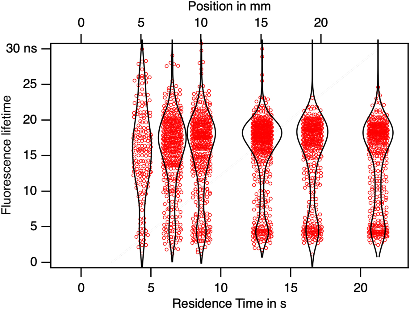
The fluorescence lifetime of individual crystals was measured at different positions along the flow. The size distributions are represented by a black profile. The distributions of lifetime exhibit two distinct populations with lifetimes of 4 ns and 19 ns corresponding to two polymorphs. Following nucleation, their proportions remain constant throughout the growth process.

4.1 Principal component analysis versus single particle detection

The principal component analysis has identified four principal components (see Figure 10). Of these components, three remain constant over time. The fluctuating component is the one associated with the flow of crystals. The long fluorescence decay of that component is as expected. But the PCA approach does not separate the two fluctuating sources, namely the crystals with a 4 ns decay and the crystals with a 19 ns decay. It appears that the difference between the two decays is below the total noise of the fluorescence signal. This difference has been lost when we have rejected the components of low importance that we have neglected as noise. PCA is not intended to see rare events.

In this sample, where individual objects can be distinguished, it is possible to select photons of interest and reject the majority of background photons. This allows the difference between the two polymorphs to be observed.

However, the single particle approach requires a sensitivity and a resolution that is not always available. In contrast, PCA is capable of operating at the best of the possibility of the signal-to-noise ratio.

4.2 Observation of the birth of a crystal

The signal-to-noise ratio in this experiment is compromised by the presence of a significant signal with a very short lifetime. The source of the signal is the molecules in solution. They have been reported to have a fluorescence yield less that 2.10⁻³ [10]. However, this is sufficient to engulf the photon counts. The photon counts per crystals are typically 100 photon/s as illustrated in Figure 7, which is relatively low. The low photon counts from the crystals is attributed to the absorption of the excitation light by the free molecules. After the nozzle, the saturated solution (33.10⁻³ mol/L) expends over a diameter of 100 µm. The absorbance of that tube at 343 nm is 5. Thus, most of the excitation light is absorbed by the peripheric molecules and few reaches the crystal formed at the centre of the flow. This explains the difficulty to detect the nuclei. For further work there is a need to find a molecule that turns fluorescent in the solid states but that does not absorb light at the excitation wavelength of the crystal.

The pitfall in merging an epifluorescence microscope, a single photon counting apparatus, a microfluidic device, pumps, valves, metastable solutions is that the probability that everything works at the same time tends to zero. Our experience with LINCam is that is a reliable system. It can be turn on in the dark allowing sufficient time for the experimenter to adjust all the other elements of the experiment. Furthermore, the available information is stored in the form of a list of photon stream. Thus, multiple analysis and post-treatment can be performed on a single recording. A minimum of treatments are done in real time: Decay, Image, FLIM and Intensity. They give a glimpse of the data to optimize the acquisition conditions. But all possible analysis can be done later.

References

[1] J. Shi, et al.., “Multi-size control of homogeneous explosives by coaxial microfluidics,” React. Chem. Eng., vol. 6, no. 12, pp. 2354–2363, 2021. https://doi.org/10.1039/d1re00328c.Suche in Google Scholar
[2] Q. Shi, H. Chen, Y. Wang, J. Xu, Z. Liu, and C. Zhang, “Recent advances in drug polymorphs: aspects of pharmaceutical properties and selective crystallization,” Int. J. Pharm., vol. 611, p. 121320, 2022, https://doi.org/10.1016/j.ijpharm.2021.121320.Suche in Google Scholar PubMed
[3] M. Durelle, F. Gobeaux, T. K. Truong, S. Charton, and D. Carriere, “Measurement of nucleation rates during nonclassical nucleation of cerium oxalate: comparison of incubation-quenching and in situ X-ray scattering,” Cryst. Growth Des., vol. 23, no. 8, pp. 5631–5640, 2023. https://doi.org/10.1021/acs.cgd.3c00305.Suche in Google Scholar
[4] D. Erdemir, A. Y. Lee, and A. S. Myerson, “Nucleation of crystals from solution: classical and two-step models,” Accounts Chem. Res., vol. 42, no. 5, pp. 621–629, 2009. https://doi.org/10.1021/ar800217x.Suche in Google Scholar PubMed
[5] Z. Zhang, et al.., “Thermodynamics of oiling-out in antisolvent crystallization. I. Extrapolation of ternary phase diagram from solubility to instability,” Cryst. Growth Des., vol. 24, no. 1, pp. 224–237, 2024. https://doi.org/10.1021/acs.cgd.3c00916.Suche in Google Scholar
[6] Z. Zhang, et al.., “Thermodynamics of oiling-out in antisolvent crystallization. II. Diffusion toward spinodal decomposition,” Cryst. Growth Des., vol. 24, no. 8, pp. 3501–3516, 2024. https://doi.org/10.1021/acs.cgd.4c00231.Suche in Google Scholar
[7] N. Candoni, R. Grossier, M. Lagaize, and S. Veesler, “Advances in the use of microfluidics to study crystallization fundamentals,” Annu. Rev. Chem. Biomol. Eng., vol. 10, pp. 59–83, 2019, https://doi.org/10.1146/annurev-chembioeng-060718-030312.Suche in Google Scholar PubMed
[8] A. Y. Lyubimov, et al.., “Capture and X-ray diffraction studies of protein microcrystals in a microfluidic trap array,” Acta Crystallogr. D Biol. Crystallogr., vol. 71, no. 4, pp. 928–940, 2015. https://doi.org/10.1107/S1399004715002308.Suche in Google Scholar PubMed PubMed Central
[9] J. Jang, W.-S. Kim, T. S. Seo, and B. J. Park, “Over a decade of progress: crystallization in microfluidic systems,” Chem. Eng. J., vol. 495, p. 153657, 2024, https://doi.org/10.1016/j.cej.2024.153657.Suche in Google Scholar
[10] J. Shi, et al.., “Solid state luminescence enhancement in π-conjugated materials: unraveling the mechanism beyond the framework of AIE/AIEE,” J. Phys. Chem. C, vol. 121, no. 41, pp. 23166–23183, 2017. https://doi.org/10.1021/acs.jpcc.7b08060.Suche in Google Scholar
[11] V. L. Tran, et al.., “Nucleation and growth during a fluorogenic precipitation in a micro-flow mapped by fluorescence lifetime microscopy,” New J. Chem., vol. 40, pp. 4601–4605, 2016, https://doi.org/10.1039/c5nj03400k.Suche in Google Scholar
[12] I. Mejri, T. Kouissi, A. Toumi, N. Ouerfelli, and M. Bounaz, “Volumetric, ultrasonic and viscosimetric studies for the binary mixture (1,4-dioxane + water),” J. Solution Chem., vol. 50, no. 9, pp. 1131–1168, 2021. https://doi.org/10.1007/s10953-021-01109-z.Suche in Google Scholar
[13] H.-J. Chang, et al.., “Refractive index measurements of liquids from 0.5 to 2 µm using Rayleigh interferometry,” Opt. Mater. Express, vol. 14, no. 5, pp. 1253–1267, 2024. https://doi.org/10.1364/OME.519907.Suche in Google Scholar
[14] S. J. Yoon, et al.., “Multistimuli two-color luminescence switching via different slip-stacking of highly fluorescent molecular sheets,” J. Am. Chem. Soc., vol. 132, no. 39, pp. 13675–13683, 2010. https://doi.org/10.1021/ja1044665.Suche in Google Scholar PubMed
[15] A. D. Edelstein, M. A. Tsuchida, N. Amodaj, H. Pinkard, R. D. Vale, and N. Stuurman, “Advanced methods of microscope control using µManager software,” J. Biol. Methods, vol. 1, no. 2, 2014, https://doi.org/10.14440/jbm.2014.36.Suche in Google Scholar PubMed PubMed Central
[16] J.-A. Spitz, et al.., “Scanning-less wide-field single-photon counting device for fluorescence intensity, lifetime and time-resolved anisotropy imaging microscopy,” J. Microscopy, vol. 229, no. Pt 1, pp. 104–114, 2008. https://doi.org/10.1111/j.1365-2818.2007.01873.x.Suche in Google Scholar PubMed
[17] “Learn how to use HDF5” HDFGroup. Available at: www.hdfgroup.org.Suche in Google Scholar
[18] Wikipédia, “Écoulement de Poiseuille – Wikipédia, l’encyclopédie libre,” Available at: http://fr.wikipedia.org/w/index.php?title=écoulement_de_Poiseuille Accessed: Oct. 24, 2024.Suche in Google Scholar
[19] H. J. Kim, D. R. Whang, J. Gierschner, C. H. Lee, and S. Y. Park, “High-contrast red-green-blue tricolor fluorescence switching in bicomponent molecular film,” Angew Chem. Int. Ed. Engl., vol. 54, no. 14, pp. 4330–4333, 2015. https://doi.org/10.1002/anie.201411568.Suche in Google Scholar PubMed
[20] Z. Zhang, et al.., “Burning TADF solids reveals their excitons’ mobility,” J. Photochem. Photobiol. A Chem., vol. 432, no. 1, p. 114038, 2022. https://doi.org/10.1016/j.jphotochem.2022.114038.Suche in Google Scholar
[21] I. T. Jolliffe and J. Cadima, “Principal component analysis: a review and recent developments,” Philos. Trans. A Math. Phys. Eng. Sci., vol. 374, no. 2065, p. 20150202, 2016. https://doi.org/10.1098/rsta.2015.0202.Suche in Google Scholar PubMed PubMed Central
[22] N. G. Van Kampen, Stochastic Processes in Physics and Chemistry, 3rd ed. North Holland, Elsevier Science Publishers B.V., 1992.Suche in Google Scholar
[23] A. A. Chernov, Modern Crystallography III, Crystal Growth, Berlin, Springer, 1984, p. 842.10.1007/978-3-642-81835-6Suche in Google Scholar
[24] A. W. Bowman and A. Azzalini, Applied Smoothing Techniques for Data Analysis, London, Oxford University Press, 1997.10.1093/oso/9780198523963.001.0001Suche in Google Scholar
© 2025 the author(s), published by De Gruyter on behalf of Thoss Media
This work is licensed under the Creative Commons Attribution 4.0 International License.
Artikel in diesem Heft
- Frontmatter
- Editorial
- Embracing the power of fluorescence lifetime imaging
- News
- Community News
- Views
- Perspective: fluorescence lifetime imaging and single-molecule spectroscopy for studying biological condensates
- Advanced fluorescence lifetime-enhanced multiplexed nanoscopy of cells
- Tutorials
- From principles to practice: a comprehensive guide to FRET-FLIM in plants
- Fluorochrome separation by fluorescence lifetime phasor analysis in confocal and STED microscopy
- Calibration approaches for fluorescence lifetime applications using time-domain measurements
- FRET-analysis in living cells by fluorescence lifetime imaging microscopy: experimental workflow and methodology
- Protocol for in vivo fluorescence lifetime microendoscopic imaging of the murine femoral marrow
- Research Articles
- Spectro-FLIM for heritage: scanning and analysis of the time resolved luminescence spectra of a fossil shrimp