Spectro-FLIM for heritage: scanning and analysis of the time resolved luminescence spectra of a fossil shrimp

2.1 The fossil specimen

The specimen of A. longirostrus studied consists of two slabs (imprints and counter-imprints) collected from a new site in Idaho (USA) containing the Paris Biota. The specimen is studied jointly by Biogéosciences and the PPSM in the context of an 80prime project from the CNRS (2023–2027). The two slabs show an intriguing distinct luminescence under UV light, the one studied here exhibiting a white-blue luminescence (repository number UBGD.301002.1, Université de Bourgogne, Géologie Dijon; Figure 1), while on the other slab the shrimp remains show a yellowish luminescence. Previous studies using mid-infrared spectral imaging (FT-IR mode) revealed that crustacean fossils from the Paris Biota consist mainly of hydroxyapatite with a minor contribution from calcite [3]. Raman analysis also suggested the presence of organic remains [3]. UBGD.301002.1 is well suited to the development of FLIM imaging because of its high brightness, the nanosecond decay time of the constitutive minerals and its relative flatness.

Figure 1:

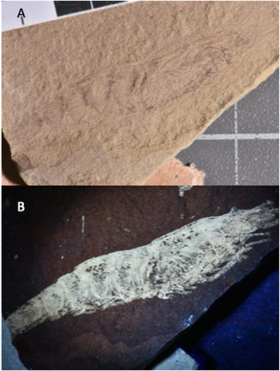
Sample containing a shrimp Anisaeger longirostrus (inv. no. LAKBPB2B8): room light observation (A), fluorescence image under UVB excitation (B). Note the bright luminescence that allows tiny organs to be seen against a dark background.

2.2 Setup

Excitation is performed using the third harmonic (343 nm) of an ytterbium tungstate laser (Goji, Amplitude, Pessac, France). The laser repetition rate of the laser employed was 10 MHz. The laser power reaching the sample is below 10 µW.

The inverted epifluorescence microscope is a TE2000-U from Nikon equipped with an objective “Plan Fluor 10X” with a limited transparency at 343 nm (40 %), a field of view of 2,200 µm in diameter, a numerical aperture of 0.30 and a working distance of 16 mm. The additional magnification of the relay lenses (×5) in front of the 22 mm detector results in a the FLIM field of view of c.a. 450 µm.

The single photon counting camera (LINCam, Photonscore GmbH, Magdeburg, Germany; version produced in 2007) was used for detection [4].

The sample is excited along a stripe and the fluorescence is collected along a slit (Figure 2). This beam from the slit is dispersed by a grating and imaged on the surface of the detector. The fluorescence spectra and decays from each point of the stripe is recorded. The surface of entire fossils can be raster-scanned. The excitation slit is useful for the alignment of the cylindrical lens and can be removed. The detection slit can act as a confocal pinhole. The focussed excitation beam provides a Z sectioning of 17.2 µm of the collected fluorescence in a transparent sample. It can be a 450 µm slit that collect both the direct fluorescence and the scattered fluorescence from the sample. With the larger slit we lose spectral resolution, but we are more sensitive, which allows decreasing the flux to reduce potential damages to the specimen.

Figure 2:

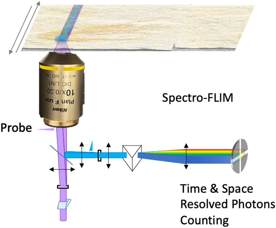
Scheme of the line confocal and spectrograph organization of the epifluorescence setup in front of the time and space resolved single photon counting LINCam. The excitation beam is focused along a stripe with a cylindrical lens. The image of the fluorescence stripe on the side port of the microscope is dispersed by a grating. The image of the spectrum is done on the photocathode of the LINCam.

2.3 Excitation optics

2.3.1 Lighting along a stripe

In order to collect more light in the spectrometer, a cylindrical lens was positioned upstream from the microscope to transform the circular beam into a slit-shaped beam (Figure 3).

Figure 3:

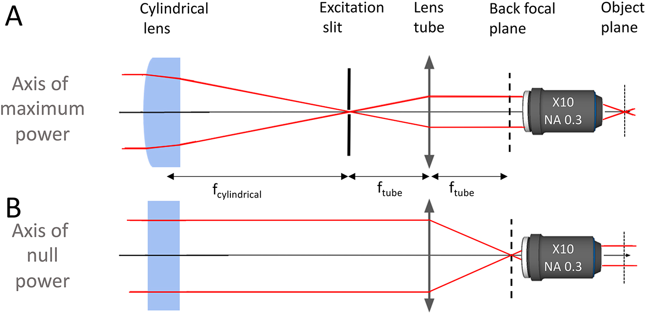
Propagation of the beam in the configuration used for imaging the fossil: in the axis of maximum power of the cylindrical lens (top), and in the axis of null power (bottom). A slit was added to the setup at the focal point of the cylindrical lens to filter the laser excitation profile.

Since the emitted radiation is also filtered by a slit of 150 µm in the set-up proposed here, we have constructed an anamorphic confocal microscope. The axial resolution was quantified by measuring its point spread function (PSF) with the view to characterizing its confocal performance.

2.3.2 Depth of field and resolution

The images of a ϕ = 1 μm rhodamine latex bead was recorded at varying heights Z of the objective. Figure 4 shows the intensity of the bright spot integrated over its area as well as the variance of the Gaussian fit of the spot as a function of Z. At large defocus, the presence of a second bead in the field perturbs the recording.

Figure 4:

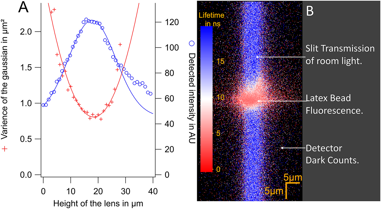
Measurement of the resolution of the slit confocal setup. (A) Number of photons detected for the bead as a function of the height Z of the focal point/the microscope lens (blue circle). The FWHM gives the depth of field of the confocal setup. FWHM = 14.3 ± 0.4 μm with an emission slit of 150 µm. The red crosses are the squared widths of the Gaussian fit of the images of the latex bead as function of the position of the lens. The minimum gives the lateral resolution of the detection path. (B) Image of the latex bead behind the emission slit. The colour codes for the lifetime. A few ns for the bead, 40 ns for room light.

The minimal radius, ω₀ = 2σ₀ = 1.62 ± 0.03 µm, is obtained by fitting the width as a function of the height Z:

ω 2 Z = ω 0 2 + λ π ω 0 2 Z 2

2σ₀ is the spatial resolution provided by the detection path.

The depth of field of the excitation beam is deduced from the plot of the intensity as a function of Z to be FWHM = 17.2 ± 0.7 μm.

In the following work, an emission slit with a width of 340 µm was used. This large slit is chosen to fit the width of the scattering of the fluorescence by the sample. The scattering and the use of this large slit preclude the possibility of achieving resolution in depth with this particular sample.

2.4 Emission optics

The fluorescence signal is collected by the microscope (TE2000-U, Nikon) and imaged to the side port (Figure 5). Fluorescence anisotropy measurements can be made using a Glan-Thomson prism and a pentaprism [4]. The image has a diameter of 7 mm with a numerical aperture of 10⁻² rad. This image is transferred towards the photocathode of the LINCam, situated 1.5 m away by two lenses with a fivefold magnification. The first lens collimates the beam. Optionally it can be reflected onto a grating by two mirrors. The grating then creates a vertical dispersion of the light. In the latter configuration, a horizontal slit whose height can be mechanically adjusted, is placed in the intermediate plane at the exit of the microscope. As a result, the detector is covered by a family of spectra. The reflection by the two mirrors adds 70 mm to the distance between the two lenses. This has a negligeable impact on the focus of the image on the LINCam, but the image of the slit is flipped horizontally. It is essential to ensure that the angular adjustment of the grating is precise (typically 3.10⁻⁶ rad) due to the distance between the grating and the photocathode.

The magnification at the photocathode is measured to be 1.006 µm/pixel using a “1951 USAF Resolution Test” target.

The dispersion of the grating is constant and is measured to be 2.6838 pixel/nm at the photocathode using a five wavelengths dichroic filter (ZET405/445/514/561/640×, Chroma, Bellows Falls USA).

The grating position and the offset of the spectrum on the photocathode are calibrated with the same filter.

Figure 5:

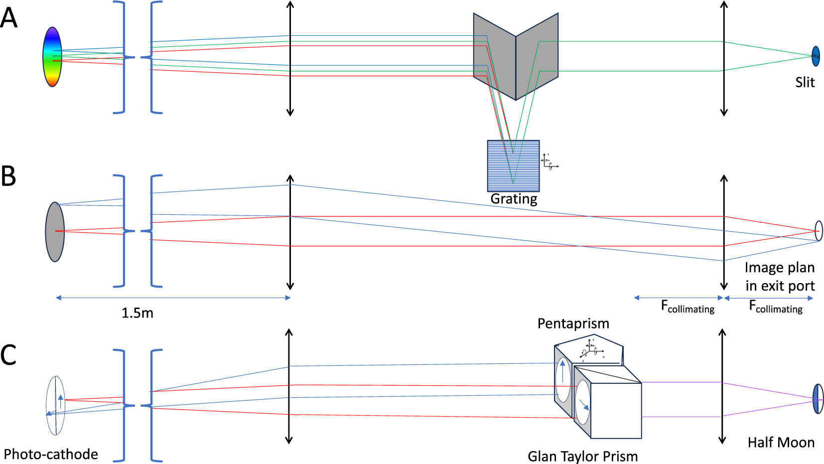
Expansion scheme using two lenses to adjust the size of the image produced by the microscope to that of the detector (center). The first lens is placed at a distance equal to its focal length, so that any point source in the microscope image forms a collimated beam that will reach the grating at the same angle. The beam is sent towards the grating and collected by two mirrors (top). These mirrors can be inserted and removed using a translation stage. The angle of the grating requires fine, reproducible positioning.

2.5 Sensitivity

Determining the absolute sensitivity of the detection (number of photons collected per photon emitted) is beyond the scope of this paper. However, we have compared the spectral data collected (with the LINCam detector) with a conventional spectrograph (MAYA Pro, Ocean Optics, Duiven, Netherlands). The same excitation power was used for both acquisitions (7 µW). The spectra were collected for 100 ms and averaged over 10 s for the MAYA Pro detector and over 60 s on the LINCam detector (Figure 6). These usual conditions offer the same signal to noise ratio on both instruments even the nature of their noise defers. It takes six times longer to obtain the spectrum with LINCam than with MAYA Pro. Furthermore, the compared spectra demonstrate that the spectral sensitivity is situated within the blue region of the visible spectrum for the LINCam detector, potentially overlooking the contribution of red emitters.

Figure 6:

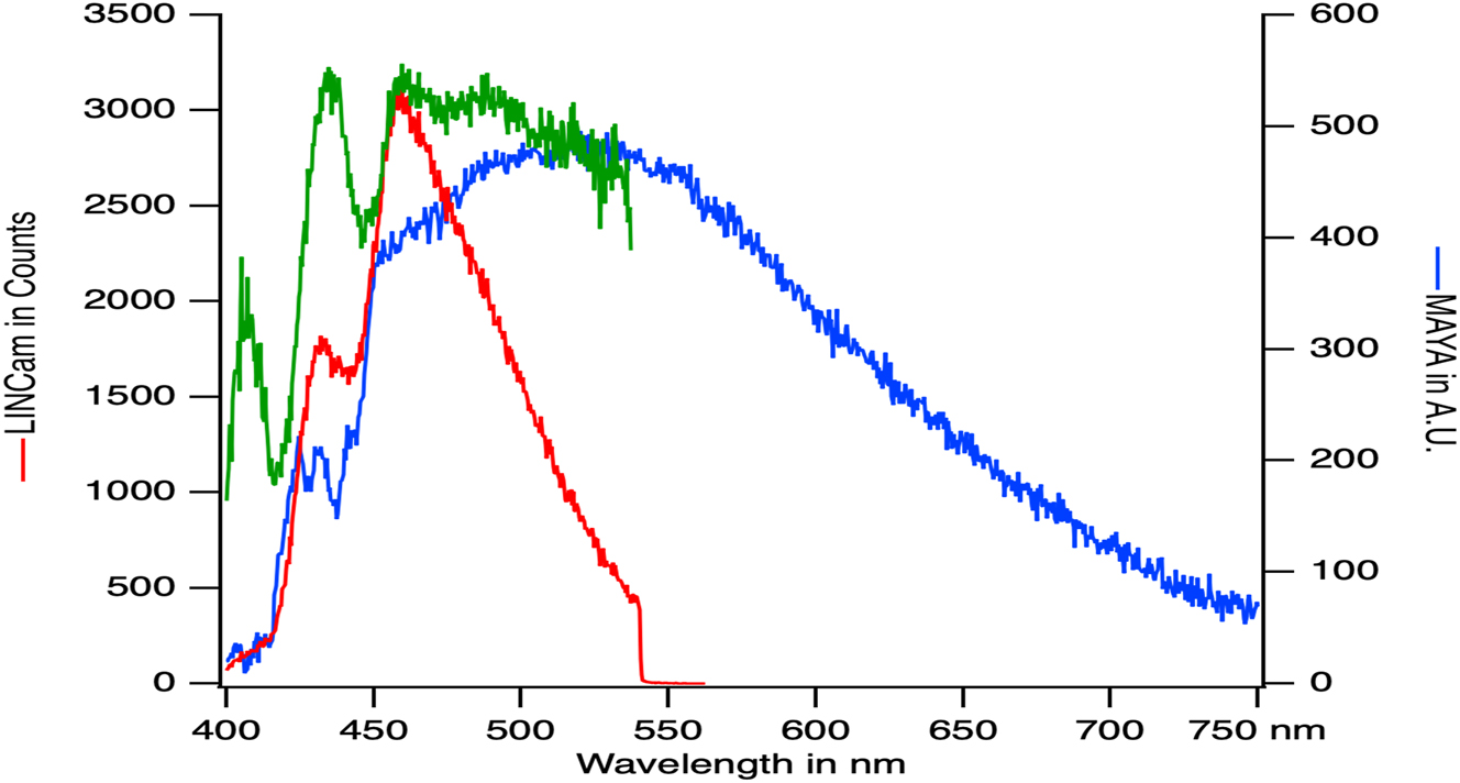
Fluorescence spectrum of the shrimp collected with the LINCam detector (red), compared to the MAYA photodiode array (blue). The spectra are not corrected for the spectral sensitivity of their detectors as a function of wavelength, which differs from one detector to another. The LINCam spectrum can be corrected for the sensitivity of the photocathode (green), but this correction does not correctly take into account the sidebands in the reflection of the dichroic mirror.

2.5.1 Spectrum correction

The production of reference data from samples requires the implementation of spectral correction. The sensitivity of the photocathode/grating ensemble depends on wavelength. The collected spectrum S λ is related to the corrected spectrum I λ by:

S λ d λ = Q E λ I λ d λ

An etalon lamp (HL-3P-Cal at 2800K, Ocean Optics, UK) was employed to calibrate: firstly the sensitivity of the MAYA Pro and secondly, the spectrum of the microscope lamp (HLX EVA 64623 at 3300K Osram Premstaetten Austria). This lamp is more intense in the blue part of the visible spectrum. Subsequently, the sensitivity of the LINCam was then calibrated using the Osram lamp (Figure 7). The correction is accurate between 450 nm and 550 nm. Below 450 nm, structures with depths of 415 nm and 445 nm are a consequence of the sidebands present in the UV dichroic mirror (Figure 6).

Figure 7:

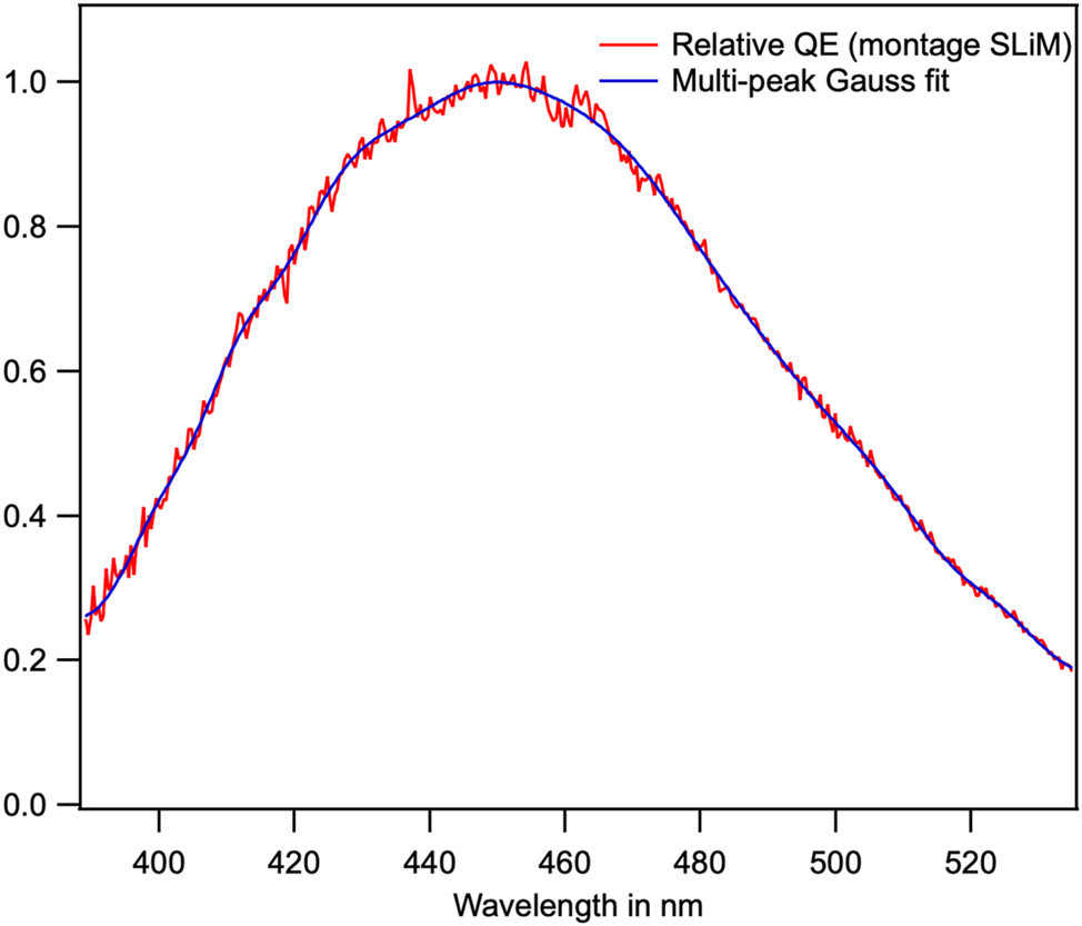
Radiant sensitivity spectrum of the LINCam photocathode in photoelectrons/W obtained by recording the spectrum of a calibrated lamp. The spectrum obtained is that of a Bialkali photocathode, which is not sensitive in the red part of the visible spectrum.

Thus, our LINCam is equipped with a Bialkali photocathode (Figure 7), which is not adequate for the investigation of mineral fluorescence across the entire visible spectrum. The advantage of a Bialkali photocathode is that it exhibits a very low dark count level. The dark count level adds a constant term and a noisy component in the decay curve. This dark count level can be easily quantified before turning on the laser or in the shadowed part of the detector (Figure 10(C)).

Figure 8:

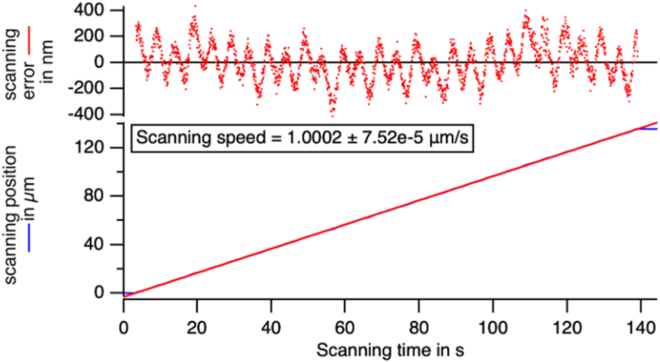
Check of the position during a scanning at a nominal rate of 1 μm/s of the translation stage. The rate is perfect and errors in the actual position during the scan stay below 0.4 μm at maximum.

Figure 9:

Large and microscopic view of the fossil shrimp in reflection. (A) The abdominal segment can be seen as dark line. The coloured spots are the locations of the point studies. (B) At the scan magnification (10× objective): the fluorescent material consists in microcrystal typically 10 µm is size. Scattering by the sample in strong.

Figure 10:

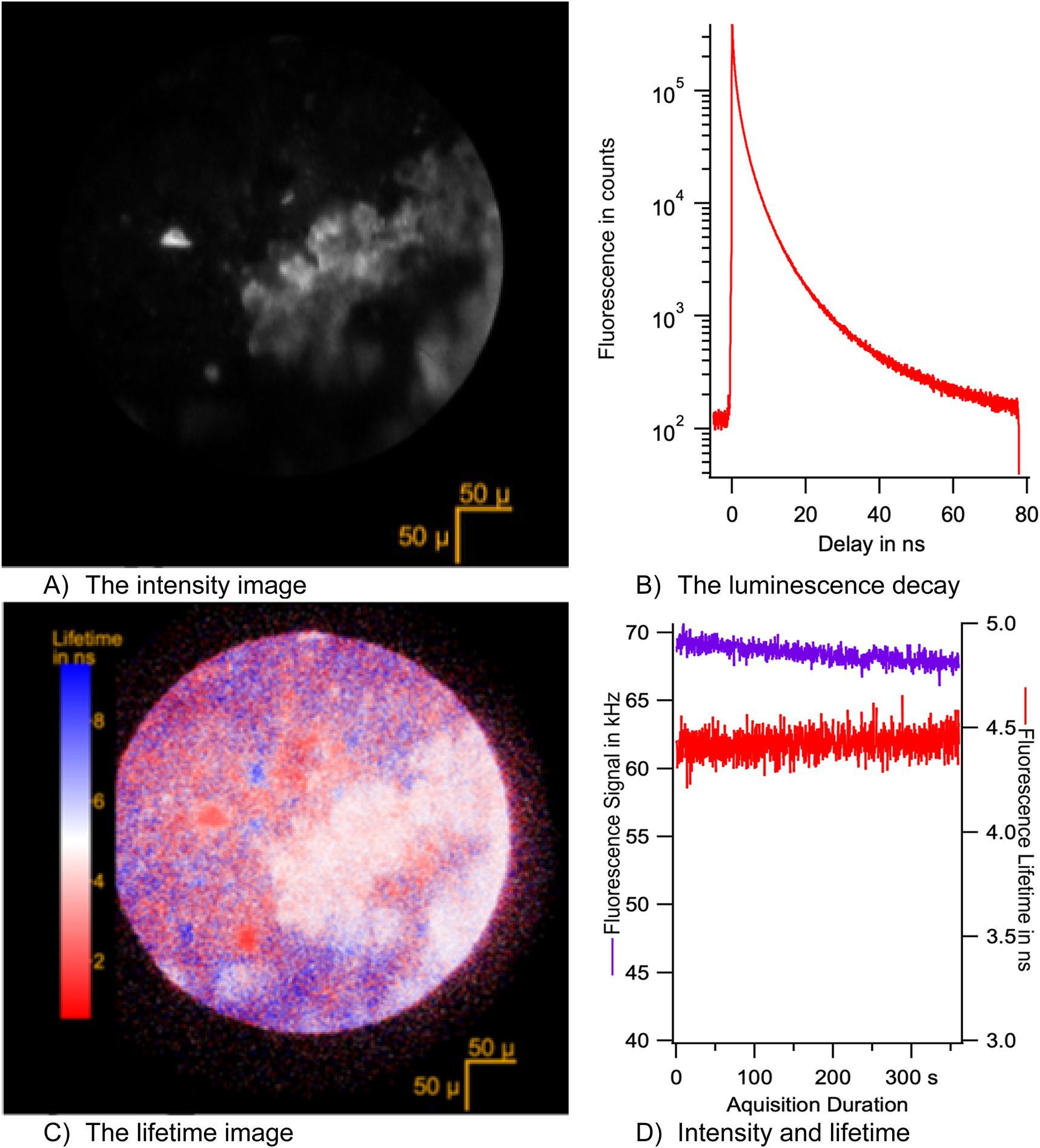
FLIM collection on the sample at position X: 6,597 µm; Y: –2,600 μm at a place corresponding to a frontier between the sediment and the fossil. Collimated illumination of 0.07 mW at 343 nm through a 10× objective for 6 min. (A) Intensity image, histogram of the photons collected per pixel (binning to 512 × 512 pixels). (B) Fluorescence decay. The histogram of the number of photons collected after the excitation by a laser. The photons have been binned over 3,584 channels. The photons from all over the image are gathered for this first analysis. The multiexponential decay observed is usual in solids. (C) FLIM image. The short-lived crystals appear in red. The dominant phase appears in white. The dark areas of the intensity image appear randomly red and blue because of the noisy estimate of the lifetime. Points outside of the shined area are dark counts of the photocathode. (D) Fluorescence intensity and average lifetime along the recoding.

2.6 Scanning

A motorized scanning stage (SCAN IM 100 × 40 – 1 mm, Märzhäuser, Wetzlar, Germany) was used to perform a raster scan of a 10 µm stage micro-meter. As the precision in the scanning rate is of critical importance in our application, we have recorded the movement of a target at a speed of 1 μm/s over 135 s. Image registration in the direction of the movement was performed on successive images. The resulting speed measurement was 1.0002 ± 0.0007 μm/s and the range of the oscillations of the real position with respect to the expected one was below 0.4 µm (Figure 8). The scanning range of the stage (8 cm) and the precision of the scanning rate fit the requirment of the sample that is 6 cm long and composed of 10 μm grains (Figure 9)

2.7 Reconstruction of the image

All calculations were performed using the Igor Pro work environment (WaveMetrics, Lake Oswego, Oregon, USA).

Each photon is stored with at least four values: its X and Y positions on the photocathode, its TAC (time between the laser arrival and the photon detection, the fluorescence delay), and its TAbs (time from the beginning of the recording). The X and Y positions are encoded between 0 and 4,096 digits, which suits the resolution of the position measurement on the photocathode. To reduce processing time and memory usage, the image size was reduced to 512 × 512 pixels. The effective number of channels used to collect the luminescence decay (TAC values) is 3,584.

In scanning mode, Y codes for the wavelength λ:

where dispersion is the dispersion of the light by the grating in pixel/nm,

TAbs codes for the position PosY in the sample through:

where ScanSpeed is in m/s, resolution is in m/pixel and FreqTAbs is the frequency of the clock that measures TAbs, the time from the beginning of the recording. FreqTAbs = 10⁸ Hz.

Data processing is all about histograms, i.e. projections of these 4D data sets into 1D or 2D representations.

The fluorescence image is the number of photons collected as a function of the pixel position on the sample (PosX, PosY):

where δ_i,X,TAbs equals 1 if the photon i falls in the pixels [X, X + Binning] and at position [PosY, PosY + Binning] where Binning is the binning level of the image. PosY is given by the previous relation. For a given pixel defined by PosX, PosY or X, TAbs, ∑ _i δ_i,X,TAbs is the number of photons counted on that pixel.

The fluorescence lifetime image is obtained by calculating for each pixel of the sample PosX, PosY the ratio at any pixel:

For a given pixel defined by PosX, PosY or X, TAbs, FLIM PosX , PosY is the average fluorescence delay of the photons counted on that pixel.

The mean spectrum image λ mean is obtained by calculating, for each pixel (X, Y), the ratio:

For a given pixel defined by PosX, PosY or X, TAbs, λ mean PosX , PosY is the average wavelength of the photons counted on that pixel.

The FLIM and mean spectrum image are never infinite even when no photons are detected since in that case the numerator is undefined. Both expressions generate a noisy estimate when few photons are counted (Figure 10(C)). The Intensity image and the FLIM or spectral image can be combined into an RGB image where the brightness is given by the fluorescence intensity and where the lifetime or mean spectrum is encoded by the color. The RGB image Aquarelle is composed of three layers containing the contribution of the Red, Green and Blue of each pixel.

where RGB run through the three layers of the RGB image Aquarelle. ColorTable[,] chose a color based of FLIM in a color table. γ is the gamma correction of the intensity image. Examples of Aquarelle representations are shown in Figure 11. We used standard LUTs (Look up table) that are more colorful. We could have used bias-free tables with constant brightness for the eye also available in Igor [5].

Figure 11:

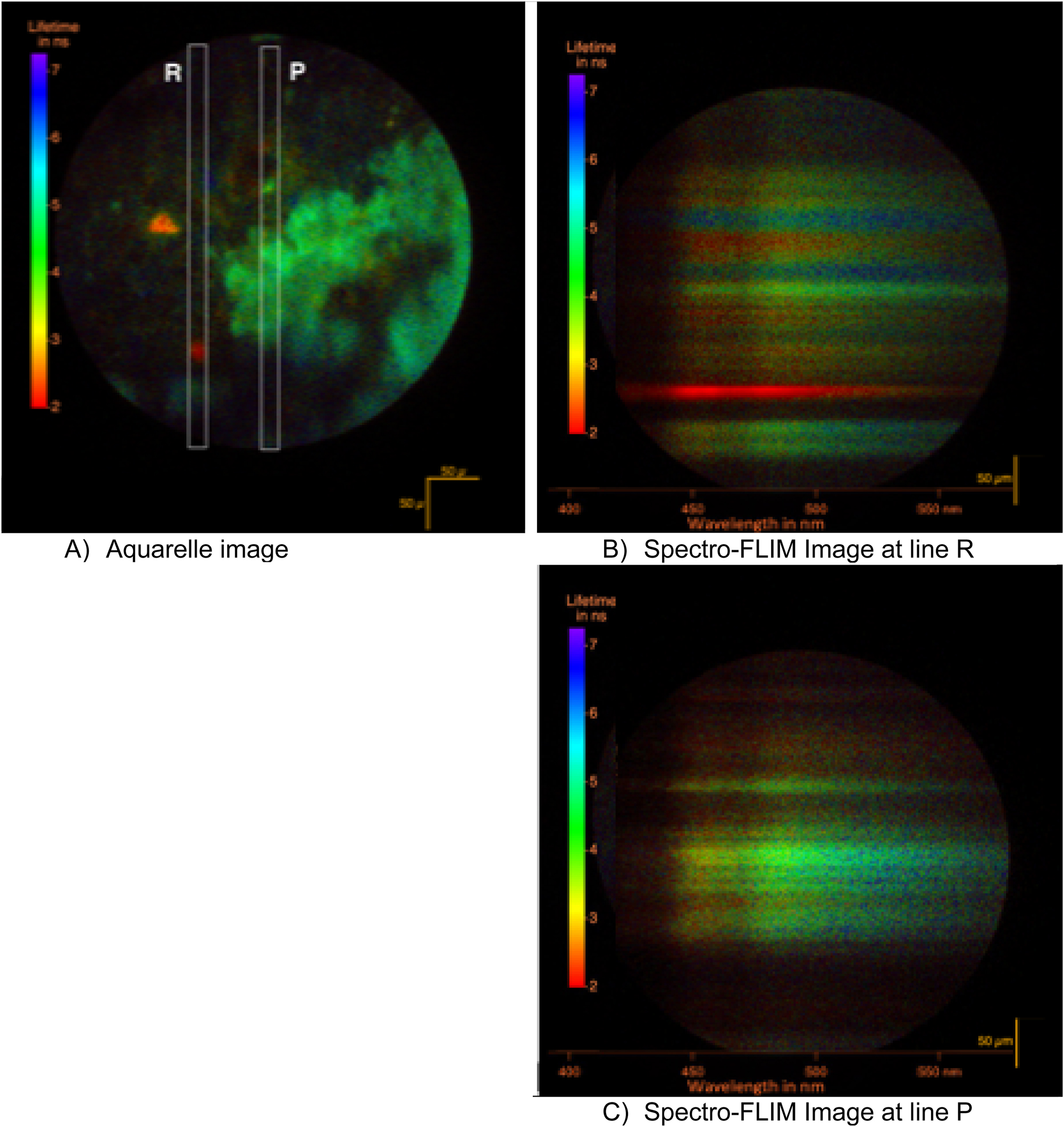
FLIM collection of the fossil LAKB2B8 at position X: 6,597 µm; Y: −2,600 µm; collimated shining of 0.07 mW at 343 nm through a 10× objective for 6 min. In (A) the aquarelle image where the brightness codes for the intensity and the color codes for the lifetime. The two short-lived crystals are more clearly seen. In (B) and (C) the slit of 10 nm in spectral width is inserted to select two positions in the previous image. The grating is put into action. Time resolved spectra are recorded. The spectral images are rotated clockwise for a better reading.

3.1 The sample

The luminescent material of UBGD.301002.1 is constituted of microcrystals measuring approximately 10 µm in size. The micro-crystals occupy the fossil volume. The specimen exhibits scattering and transparency at the emission wavelength. Analysis of the fluorescence image of four individual microcrystals reveals that 80 % of the fluorescence intensity is scattered within the sample over a distance of 14 µm before being collected. The scattering observed can be that of both the excitation and the fluorescence beams.

3.2 Point analysis

Each acquisition at a specific location on the fossil can be used to generate four displays (Figure 10), as follows:

The intensity image (Figure 10(A)). The fossil specimen appears bright, whereas the sediment appears non luminescent and dark. The FLIM image reveals a dominant ‘Phase A’ with a lifetime of 5 ns and two crystals with a short lifetime that we will call ‘Phase B’ (Figure 10(B)). The fluorescence decay is complex as is usual for solid samples (Figure 10(C)) [6]. The variation in intensity during acquisition shows a 1 % bleaching of the fluorescence at 3.5 W/m² during the recording (Figure 10(D)). Bleaching does not appear to create quenchers since the fluorescence lifetime remains stable during the recording. Consequently, the bleaching can be attributed to the destruction of fluorescent centres.

The intensity and lifetime images can be combined to form an « aquarelle » image in which the A and B phases can jointly be represented (Figure 11). By adding a 340 µm wide slit on the image of the sample on the side port of the microscope (Figure 5), a part of the image is selected. That beam can be spread in a spectrum with the grating. Two further aquisitions were made on area P and R in order to collect the spectra of these two phases.

When used in the spectrograph configuration, the detector is illuminated by a spectrum. The wavelengths spread linearly from left to right as illustrated in Figure 11(B) and (C). In Figure 11(B), the bright crystal of phase B is shown, while in Figure 11(C), the phase A is depicted. The B crystal has a spectrum that peaks at 450 nm and exhibits a uniform lifetime over the wavelength range. The A domain has a spectrum that peaks at 460 nm. This specific location on the fossil (X: 6,597 µm; Y: −2,600 µm) illustrates the observations made at numerous other locations within the fossil. The fossil comprises a primary phase A with a few crystals B dispersed over it.

3.3 Raster scanning

To obtain information over a wider area, the sample was scanned in front of the slit in the spectrograph configuration across the sample. During the scan of the sample in front of the slit, time-resolved spectra were collected. The excitation beam that is focused along the stripe is as narrow as 5 µm. However, given that over half of the emission is scattered by the sample, a wider collection slit was employed. It images 30 µm of the sample and extends the spectral resolution up to 10 nm. The bimodal shape of the fluorescence spot comprising a peak of 5 µm radius with fat tails of 14 µm, suggests that the actual resolutions are better than 30 µm and 10 nm, respectively in the spatial and spectral dimensions.

3.3.1 Spectroscopic analysis of the phase A

The spectrum accumulated during a scan is the averaged spectrum over the ribbon. In Figure 12(A) Aquarelle image of time resolved spectra collected during a scan through the sample. The large number of collected photons allows a detailed analysis of the spectroscopic signatures of the phases constitutive of the fossil.

Figure 12:

In (A) the «aquarelle image» of time resolved spectra collected during a scan through the sample. In (B) the time resolved spectra collected for different time delay after the excitation. The width of the bins have been chosen so that all spectra have the same number of photons. Note the isosbestic point.

From bottom to top, the spectra coming from the points Y of the slit are displayed (Figure 11(A)). For each point (λ, Y) of the image, the intensity is that of a spectrum, and a lifetime can also be measured. As the detector is round rather than square, the spectrum is truncated. The spectral range collected extends from 420 nm to 550 nm at half-height, but is reduced to zero at the top and bottom of the detector image. Consequently, the full height of the slit is therefore not available for all spectral treatments.

The spectrum and decay collected over the ribbon bear resemblance to those of the phase A, which is the dominant phase in the fossil.

As for each photon the fluorescence delay is known, it is possible to construct spectra for different fluorescence delay times (Figure 12(B)). The delay ranges for integrating these transient spectra were selected in order to ensure that each contained the same number of photons. The presence of an isosbestic point on the family of spectra with the same area indicates that only two emissive species might contribute to the luminescence over the ribbon. Formally, this can be said that linear combinations of two spectral end members with a variable ratio are sufficient to explain the family of spectra [7]. This parsimony of the chemical composition is promising for further processing of the data.

3.3.2 Decays and spectra construction

Principal component analysis (PCA) [8], is employed for the dimensional reduction of large dataset. The isosbestic point provide only a qualitative indication of the number of species. Whereas the PCA quantifies the contribution of components or species and let us decide how many are significant. We do assume that each emission centre is characterized by a spectrum and a characteristic decay (which is not necessarily exponential). Each emission centre can therefore be defined by a map I λ , t . It would be possible to perform a PCA on these maps as it is done on images. However, spectra are only obtained from the middle of the slit, whereas the decay is correct at any point. Consequently, we perform PCA on decays at varying wavelength over the full area of the detector. We shall then check that the proposed decays are compatible with the positivity constrains on spectra.

Three tracks were collected on the specimen: two on domains of primarily phase A and one on a domain of the primarily phase B. Decays are integrated over the entire tracks, but collected at different wavelength (Figure 13).

Figure 13:

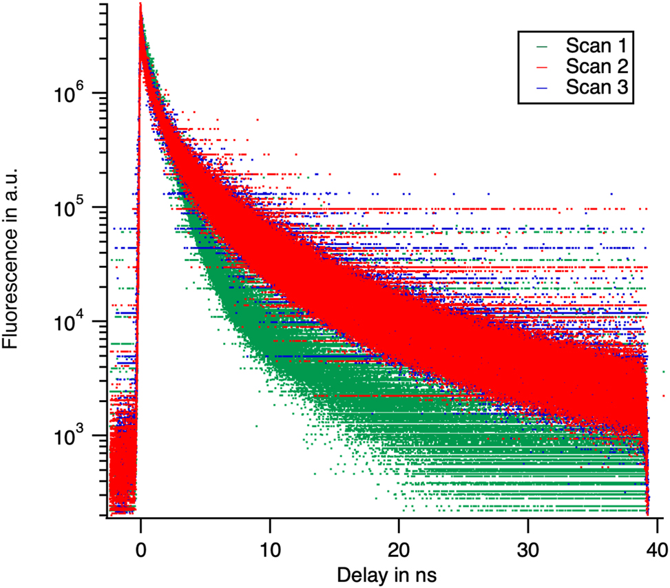
The decays used for the principal component analysis. They have been collected at successive wavelengths the decays have been normalized to the same area in the picture (not for the analysis). Note the dissimilarity between scan 1 with the other two.

Figure 14(A) displays the contribution of the principal components in the case of 59 decays collected from domains of phase A and 80 decays originating from domains of phase A and domain of phase B.

Figure 14:

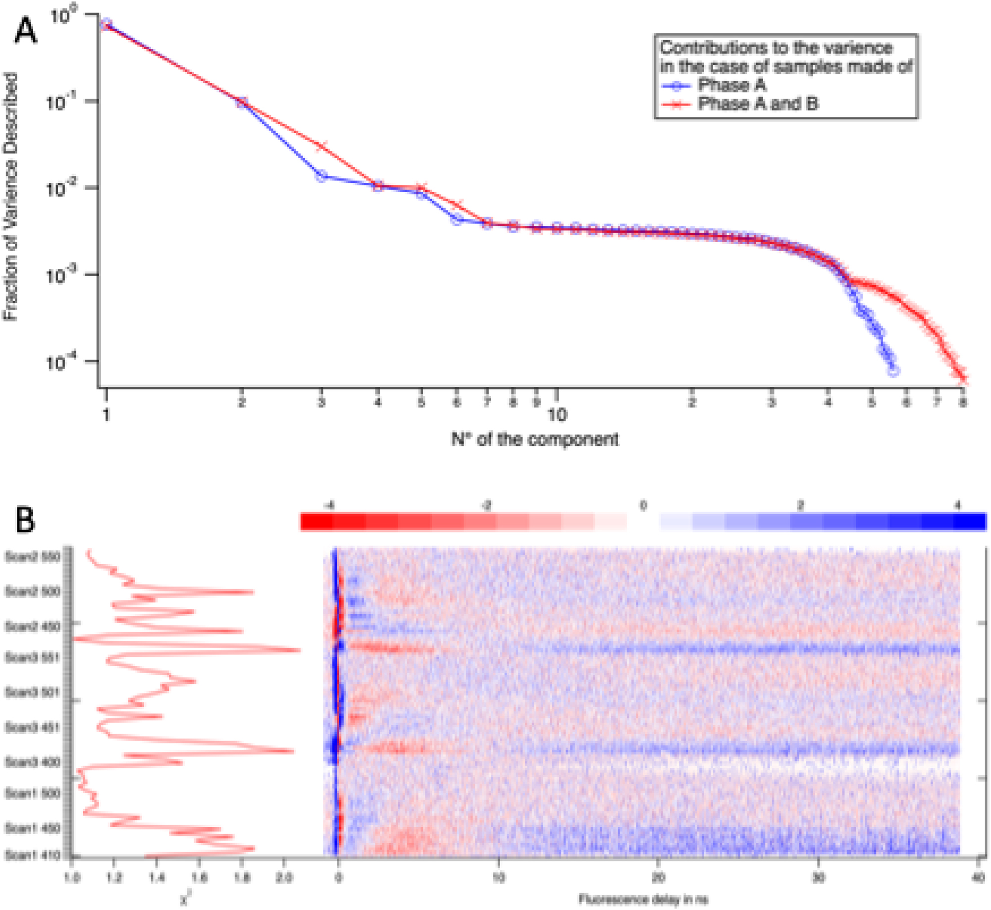
The principal component analysis provides as many orthogonal components than data. They are ordered by the fraction of the total variance of the data that they describe as shown in the top picture. The components beyond 7 describe the noise. But we keep only the first three component for practicality of the analysis. The bottom display shows the weighted difference between the data and their representation by three components. Some parts of the decay are not well described but the χ² of the error remains always between 1 and 2.

In domains of phase A, algorithm indicates that two components can describe 86 % of the variance of the data. After adding the phase B data, the same level of completeness requires three components. We shall assume that components beyond 6 describe the noise.

In this paper, we decided to neglect the components 4–6 in order to reduce the dimensionality of the reconstruction problem. The quality of the description is demonstrated by the map of the weighted residuals (Figure 14(B)). While a complete noise analysis is beyond the scope of this contribution, we propose a map showing the difference between the data and their description by the first three principal components. It helps in the identification of the problematic part of the data. The points of the map appear randomly positive and negative if the reconstructed data are within the noise of the measured data. The amplitude of the residual is estimated for each curve by the parameter χ² that has to be larger and close to 1. The data are poorly described around time 0, because of the fluctuations in the laser arrival time. The statistical analysis therefore confirms the preliminary analysis by the isosbestic point that only two emissive species are present in phase A. The third one is present in phase B.

The principal components are not the decays of the fluorescent centres. However, any linear combination of the selected principal components describes the data with the same quality. They are constraints on constructed decays. The decay of the fluorescence represents the concentration of excited states. Therefore, they must be positive at all times during the luminescence decay. Furthermore, their contribution must also be positive at all points within the sample. As they are associated with emission spectra, their contribution must be positive at all wavelengths.

However, this is not sufficient to define fully the kinetic and spectrum of the emissive defects. For instance, two kinetic models can be applied to the data. One is a direct excitation where the emission of all fluorescent centres starts from the excitation by the laser. The other is a model in which centre A2 starts from zero and is populated by an energy transfer from A1. Both models can be constructed from the principal components and describe the data equally well.

In the direct excitation model, we have chosen among the possible constructed decays, those that reach zero as soon as possible and ordered them by their lifetime. This protocol defines a unique solution. The time-dependent, decay rates of species i, that quantify the kinetics model are obtained from data by [9]:

k i t = − d L n C i t d x

In addition to the constraints of positivity of concentrations, it is general accepted that k i t must be a steadily decaying function of time t.

However, some conditions are not possible to be fulfilled based the data. It is not possible to eliminate the contribution of a decay of 840 ps in the measurement of the phase A (Figure 15). This contribution is larger than expected from the few crystals of phase B seen in Figures 11 and 17. It may come from the fact that we have neglected the Principal Components 4–6 in our analysis.

Figure 15:

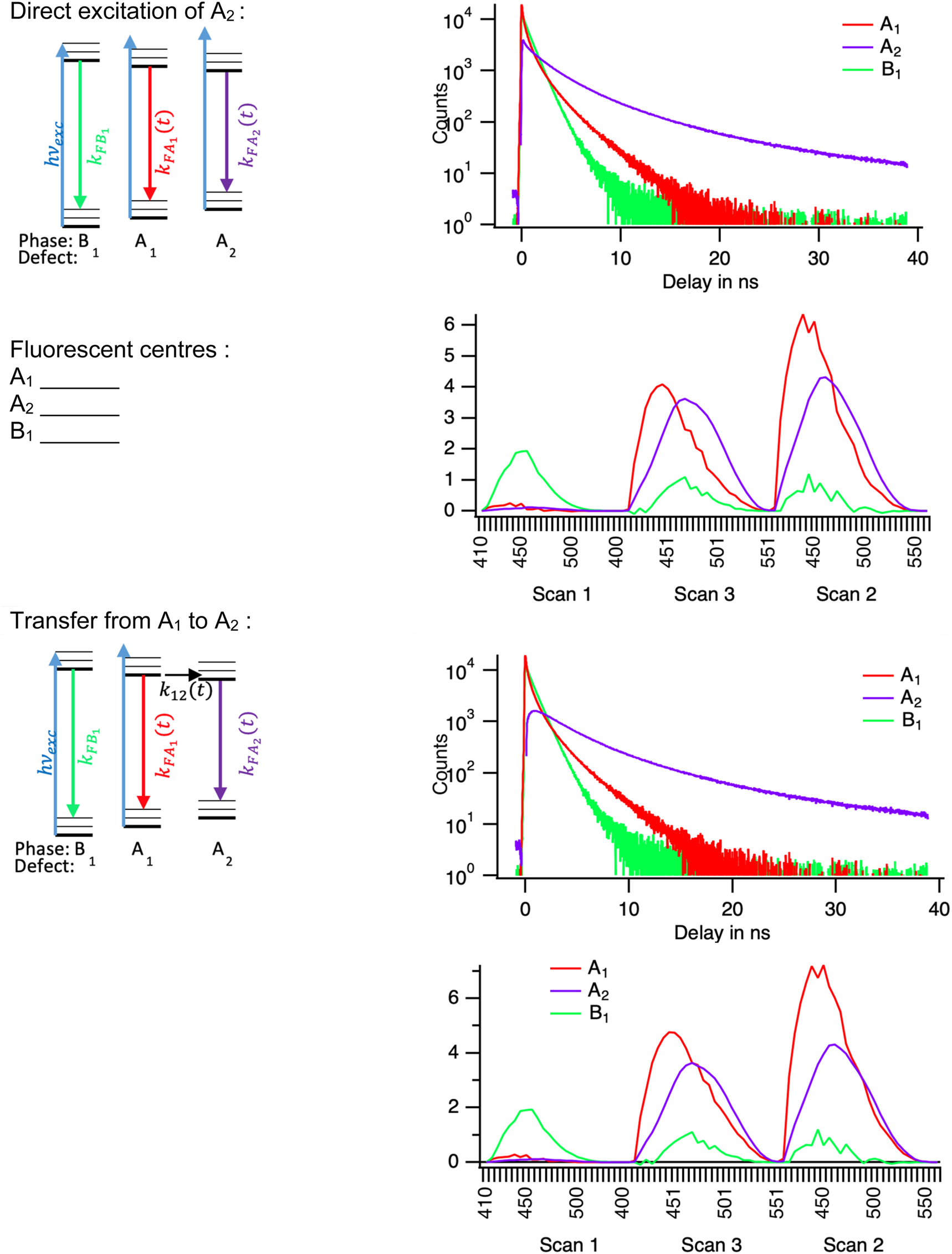
At least two models can be proposed do describe the data of the time resolved spectra: direct excitation is represented in the top half, with its Jablonsky diagram, the population decays and the species spectra. In the bottom half, the transfer model is presented.

Our data analysis is therefore neither complete (some phenomena are not described) nor sufficient (different kinetic models are still possible). However, the result of the decomposition forms a basis for further discussion of the data.

3.3.3 Image of one ribbon in the fossil

The intensity and FLIM “image” collected during the scan contains spectroscopic information but nothing about the contrasts in the specimen. A preliminary glance is given by the intensity and lifetime plot in Figure 16. The fluctuating intensity shows bright and dark areas in the shrimp. The stable lifetime suggests the predominance of the phase A. The constancy of the lifetime along the ribbon shows the uniformity of the nature of the phase A in terms of emitter ratio and of quencher concentration.

Figure 16:

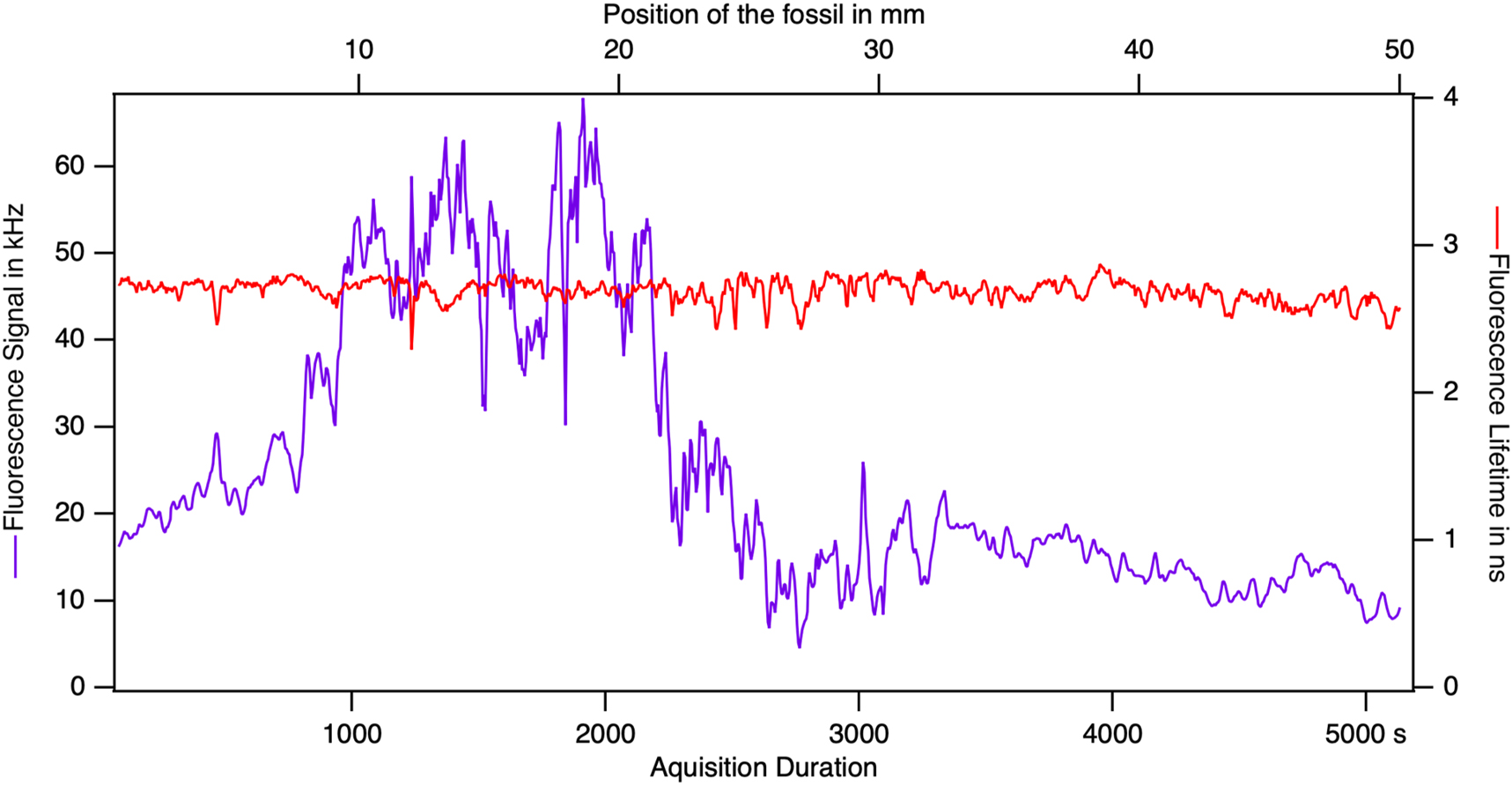
During a scan, the intensity and the lifetime along the recording gives the first hints on the results. The intensity goes through a maximum that is four times the minimum and presents sharp features. At the same time, the lifetime is very stable.

Let us now unfold the images from the scan. The decay of the luminescence can be summarised in a simplified way by the lifetime and the spectrum by the average emission wavelength, at each pixel.

4.1 Imaging performances

4.1.1 Depth of field and resolution

The optical setup described here allows the excitation of the sample along a stripe. The intensity of the excitation beam varies in Z with an FWHM of 17.2 ± 0.7 μm. The depth of field of a 2D focused beam is given by [10]:

Δ Z / 2 = 0.44 λ ex N A 2

where NA = 0.3 is the numerical aperture; λ_ex = 343 nm is the excitation wavelength.

The calculated value is 3.2 µm, which is smaller than the measured value. This is expected, given that the light flux is conserved along the focused beam. Consequently, the intensity drops more rapidly in 2D focusing than in a 1D focusing along a stripe (Figure 17).

Figure 17:

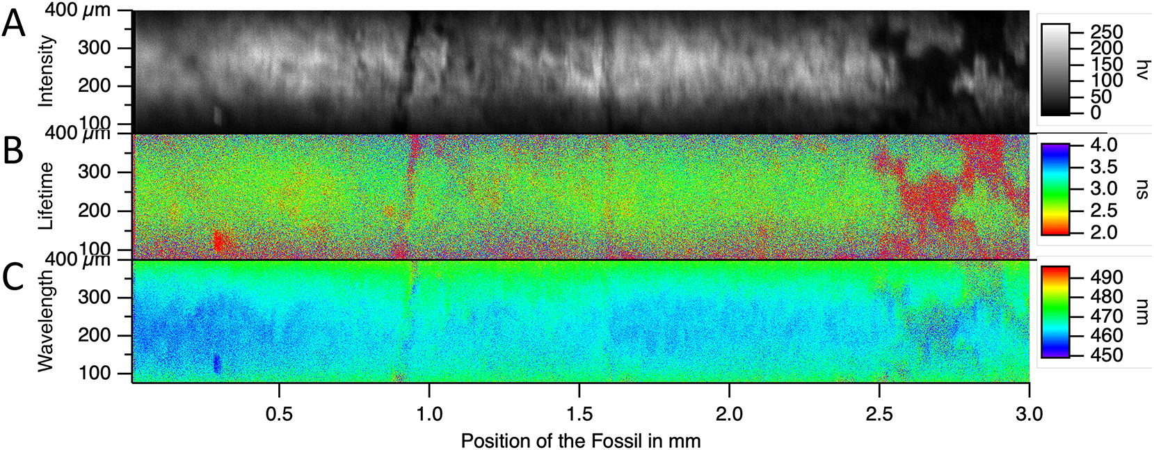
Fluorescent traces collected through the sample. (A) The intensity scanned image. (B) The FLIM scanned image. (C) The average emission wavelength scanned image.

We measured a resolution in X, Y at 570 nm in the point imaging mode with a value of ω₀ = 2σ₀ = 1.82 ± 0.03 µm. It can be calculated as [11]:

ω 0 ≅ 0.42 λ em NA

For λ_em = 570 nm, this has a value of 0.8 µm. The difference is due to the size of the latex bead.

A 340 µm slit is used to collect the light (direct and scattered fluorescence) over 34 µm of the sample. The resolution along the scan direction is defined by the size of the excitation beam and its scattering by the sample, that we have not measured. We estimate the size of the scattered beam to be 10 µm in diameter for that sample.

The wavelength resolution of the spectra is defined by the slit. 10 nm is enough for the majority of fluorescent centres with the noticeable exception of the rare earth ions that require a 1 nm resolution.

4.2 The sizing of an acquisition

The bleaching of the signal during the recording period restricts the acquisition time in many spectroscopies. Should the bleaching effect be proportional to the energy dose (and thus free from multiphotonic photochemistry and heating), it is possible to calculate this effect during a scan based on the data presented in Figure 10(D). The energy dose is proportional to the number of counted photons. In Figure 10(D) show that 2.3 % of the emitters have been lost for the collection of 24·10⁶ photons. During the scan we have collected 0.8·10⁶ photons. The transmission of the photons in the spectrograph is of the order of 10 %. Thus, 8·10⁶ photons have reached the grating. Furthermore, the lost emitters spread over a significantly larger area. In summary the lost photons during a scan ΔC_Scan are given by:

where C _o is the concentration of emitters. Δ C point C o = 2.3 ⋅ 1 0 − 2 is the fraction of emitter bleached in a point illumination. S Fixe S Scan is the ratio of the illuminated areas.

This result demonstrates that the bleaching effect is negligeable during a scanning process. The power of the excitation laser can be increased by two orders of magnitude.

A bleaching of the emitters can be seen but it is never a burning of the sample due to a local heating by a focused high-power laser [12].

If the bleaching is not a limit for the acquisition duration, then the duration of an acquisition slot during a session will be the limit. Knowing that we collect in spectral mode 30,000 photons per second, we can scan at a rate of 10 μm/s a slit with a useful height of 300 µm. The fossil fitting within a 10 cm × 2 cm frame, the acquisition time of the entire fossil will be 180 h, that is more than a week for a single sample. This requires a full automatization of the acquisition. This is possible if we can automatize the scanning and in particular the focus. Even if the sample is flat, with a 20 µm depth of field, we need to adjust the focus during the recording. In the future, for more irregular samples, we shall need to get rid of the microscope.

4.3 Spectroscopic characterisation of the emission centres

The fluorescence of the fossil has been analysed with regard to fluorescent centres. The conclusions derived from this analysis of these data are limited in scope, applying only to three tracks in a single slab of the UBGD.301002 specimen. Nevertheless, they demonstrate that, even in the presence of multi-exponential decays, conclusions can be drawn from the recording of the fluorescence lifetime Imaging (FLIM) of minerals.

Previous work using mid-IR spectroscopy (FT-IR mode) made on other fossils from the Early Triassic Paris Biota showed that they are mostly made of hydroxy-apatite and to a lesser extent of calcite, whereas Raman studies further detected the presence of organic molecules [3].

Hydroxy-apatite Ca₁₀(PO₄)₆(OH)₂ presents both an intrinsic and a doped fluorescence. The fluorescence of undoped synthetic hydroxy-apatite shows a broad emission from 400 nm to 700 nm when excited at 350 nm. The energy of the fluorescent photons is much less than the band gap of hydroxy-apatite 5.7 eV (220 nm). The luminescence does not come from the transition between the conduction band and the valence band, but from localized defects in the band gap. The nature of the luminescent defects remains unknown [13], [14].

Hydroxy-apatite can also be doped with activators of fluorescence. As said by D. K. Richter et al. [15] “It is generally accepted that Mn ²⁺ and trivalent REE-ions are the most important activators of extrinsic CL in carbonate minerals, while Fe ²⁺ is a quencher of cathodoluminescence.” The luminescences of the rare earth ions present narrow emission band and lifetime that are long compared to a few nanoseconds. The exceptions are the Cerium ions Ce³⁺ and Ce⁴⁺ that present a luminescence in the blue at 440 nm [16] and a nanosecond lifetime [17].

The construction of the decay shows that it is possible to postulate an almost exponential decay for the fluorescent defect of the phase B with a lifetime of k _f = 840 ps.

B1 emission dominates in ribbon 1 with some contribution of phase A that describes the long-lived components of the decay. This is the simplest model. Thus, from the data, it is possible to assume that the defect B1 in phase B is free of quenchers. The emission spectrum peaks at 450 nm.

For phase A, from the isosbestic point in the time resolved spectra, we assume the presence of two emitters. This describes 86 % of the variance of the data and fits the data with a χ² value lower than 2 (Figure 14). However, this does not fully fix the kinetics model. The measurement of the anisotropy of the fluorescence gives a clue. Anisotropy is the relative difference between the intensity that is collected with the same polarization than the excitation I_‖ compared to that collected perpendicular to that direction I_⊥.

The theory of fluorescence anisotropy has been fully developed for isotropic amorphous phases [18]. But it also applies for the scanning of randomly oriented micro-crystals, in particular its time resolved part.

The amplitude of the anisotropy is difficult to measure in the specimen due to the depolarization of the light by the scattering and by the dichroism of the hydroxyapatite and the calcite. However, individual crystals exhibit a non-zero anisotropy. Figure 19 shows that the anisotropy does not evolve during the fluorescence lifetime. During an energy transfer, anisotropy decreases due to the fact that acceptors are randomly oriented around the donor [19]. Indeed, hydroxy apatite and calcite belong to the hexagonal crystal family that contains an 3 fold axis of symmetry. Acceptors with their transition dipole in the plan perpendicular to the axis of symmetry will appear as isotropic for anisotropy measurements. Only energy transfer between transition moments, that are parallel to the C3 axis, will maintain the anisotropy. Thus, the stability of the anisotropy during the fluorescence lifetime is indicative of the absence of energy transfer between emitters.

We shall postulate that the two emitters A1 and A2 are independent, and we shall postulate that the A1 has the shortest possible lifetime τ A 1 and it drops to zero fluorescence as soon as possible. This is displayed on Figure 18. The decay of A1 gives a lifetime:

Figure 18:

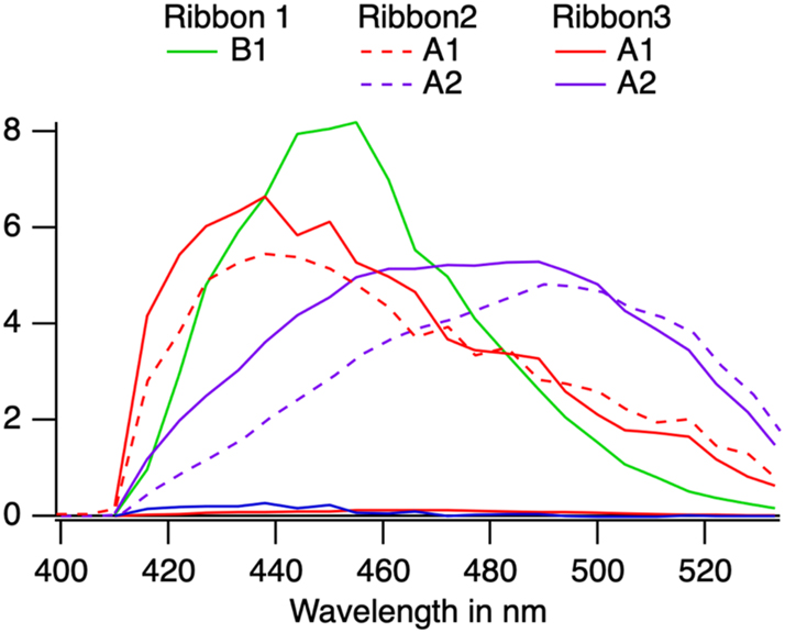
Spectra of the emitters assuming independent emissions and assigning the shortest possible lifetime for A1. The spectra are corrected for the photocathode sensitivity but in arbitrary units.

Its fluorescence peaks at 437 nm.

The second emitter then must peak at 490 nm and has a decay that exceeds the measurement window. Thus, the lifetime τ A 2 is longer than 5 ns.

Both A1 and A2 emitters have multiexponential decays. This is due to the presence of quenchers in their neighbourhood, a few quenchers at random distances [20].

Manganese ions in substitution for calcium are common emitters in calcite [21]. However they are reported to emit from 500 nm to 600 nm, which we did not observe. This may be simply because the photocathode is not sensitive at these wavelengths.

All three defects emit in the blue with a maximum at 437 nm 450 nm and 490 nm after correction of the photocathode and grating sensitivity. Emissions at these wavelengths have been reported following excitation at 350 nm. It has been proposed that these emitters are calcium vacancies, which are the most common intrinsic defects in hydroxyapatites [13] or cerium doping [16].

4.4 Point imaging versus scanning

The FLIM analysis can be performed in a fixed imaging mode, thereby producing data with a high resolution of key details. Alternatively, it can be carried out in scanning mode, where spectra and decays are jointly collected (Figure 19).

Figure 19:

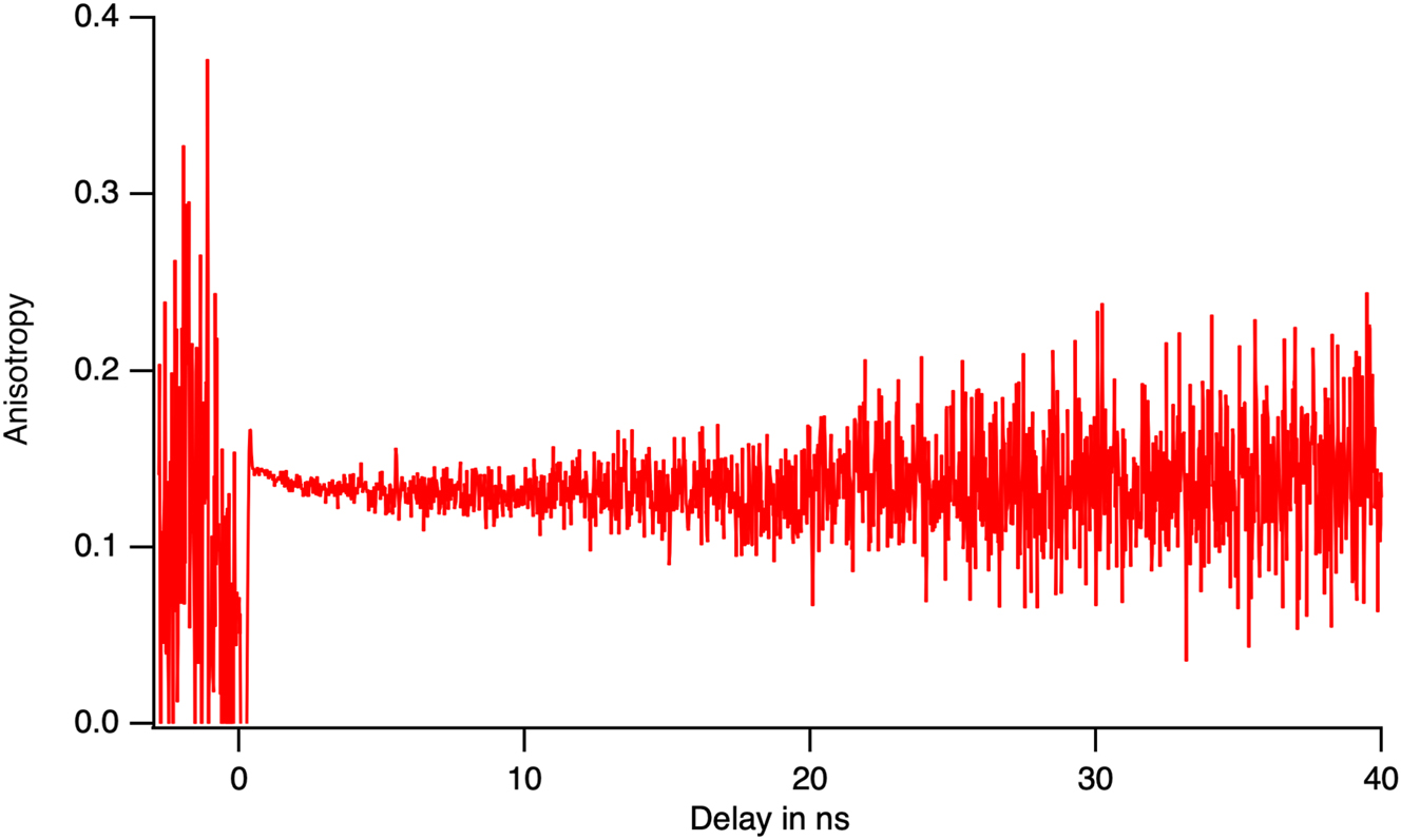
The relative difference between the emission polarisation, i.e. the anisotropy, during the lifetime of the excited state. Its stability shows the absence of energy transfer between the two emissive sites of phase A.

The scanning mode allows the quantitative analysis of a large set of points. The subsequent Principal Component Analysis of this large set of data provides the mean response and the principal variations with respect to this mean. These main variations provide the best contrasts for the image formation. Going beyond the first momentum (mean value) is particularly relevant for heterogeneous heritage samples [22]. While other approaches can be used, this method provides an optimised sparse description of imaging contrasts. The exceptions that are small in size and contribute by few photons can be smooth by the PCA. The point imaging mode allows the detection of rare by significant details such as the spare crystals of phase B present among the phase A domains.

4.5 Main results for the fossil shrimp and relevance for fossilization studies

At the wavelengths that we probed, both fluorescent vacancies and cerium dopant can be at the origin of the emission. In Phase B, we can assume a mono-exponential decay, which is rare in solids. This implies the absence of quenchers and a very pure phase. In Phase A, the decays are multiexponential, yet with a quasi-constant lifetime over the sample (Figure 16), which does not seem correlated with the concentration of iron and of other possible quenchers in the sediment. This suggests that the differentiation from the sediment and purification of the hydroxy-apatite and calcite has been extensive during the fossilization process.

Our results show that wide-field time-resolved luminescence studies can contribute to formulating rich hypotheses on the origin of luminescence emitters. The data collected provide a striking complement to macroscale luminescence imaging studies carried out on fossils from the same locality [2], [23]. Although further evidence is required to assign emission centres unequivocally, the hypotheses raised are particularly promising.

This reminds us that the detection of new sources of contrast in spectral imaging is a primary objective for the study of heterogeneous samples from cultural heritage [22], [24]. The study of regularities and correlations within fossils are often the key to the description of fossil anatomies and affinities, as it is to the understanding of micro-taphonomic pathways. This is particularly interesting when correlation can be made with detailed chemical signatures, such as the elemental ones that could be collected using XRF raster-scanning on transition metals in melanin pigments of fossil bird feathers [25] or rare earth diagenetic signatures of fossil fishes [26], [27].

References

[1] S. M. Stanley, “Estimates of the magnitudes of major marine mass extinctions in earth history,” Proc. Natl. Acad. Sci. U. S. A., vol. 113, no. 42, pp. E6325–E6334, 2016. https://doi.org/10.1073/pnas.1613094113.Suche in Google Scholar PubMed PubMed Central
[2] A. Brayard, et al.., “Unexpected early triassic marine ecosystem and the rise of the modern evolutionary fauna,” Sci. Adv., vol. 3, no. 2, p. e1602159, 2017. https://doi.org/10.1126/sciadv.1602159.Suche in Google Scholar PubMed PubMed Central
[3] M. Iniesto, C. Thomazo, and E. Fara, “Deciphering the exceptional preservation of the early triassic Paris Biota (Bear Lake County, Idaho, USA),” Geobios, vol. 54, pp. 81–93, 2019. https://doi.org/10.1016/j.geobios.2019.04.002.Suche in Google Scholar
[4] J.-A. Spitz, et al.., “Scanning-less wide-field single-photon counting device for fluorescence intensity, lifetime and time-resolved anisotropy imaging microscopy,” (in eng), J. Microsc., vol. 229, no. Pt 1, pp. 104–114, 2008. https://doi.org/10.1111/j.1365-2818.2007.01873.x.Suche in Google Scholar PubMed
[5] F. Crameri, G. E. Shephard, and P. J. Heron, “The misuse of colour in science communication,” Nat. Commun., vol. 11, no. 1, p. 5444, 2020. https://doi.org/10.1038/s41467-020-19160-7.Suche in Google Scholar PubMed PubMed Central
[6] L. Hartmann, et al.., “Quenching dynamics in CdSe nanoparticles: surface induced defects upon dilution,” (in eng), ACS Nano, vol. 6, no. 10, pp. 9033–9041, 2012. https://doi.org/10.1021/nn303150j.Suche in Google Scholar PubMed
[7] R. B. Pansu and K. Yoshihara, “Diffusion of excited bianthryl in microheterogeneous media,” (in English), J. Phys. Chem., vol. 95, no. 24, pp. 10123–10133, 1991. https://doi.org/10.1021/J100177a091.Suche in Google Scholar
[8] I. T. Jolliffe and J. Cadima, “Principal component analysis: a review and recent developments,” Philos. Trans. A Math. Phys. Eng. Sci., vol. 374, no. 2065, p. 20150202, 2016. https://doi.org/10.1098/rsta.2015.0202.Suche in Google Scholar PubMed PubMed Central
[9] M. N. Berberan-Santos, E. N. Bodunov, and B. Valeur, “Mathematical functions for the analysis of luminescence decays with underlying distributions 1. Kohlrausch decay function (stretched exponential),” Chem. Phys., vol. 315, nos. 1–2, pp. 171–182, 2005. https://doi.org/10.1016/j.chemphys.2005.04.006.Suche in Google Scholar
[10] C. J. R. Sheppard, “Depth of field in optical microscopy,” J. Microsc., vol. 149, no. 1, pp. 73–75, 1988. https://doi.org/10.1111/j.1365-2818.1988.tb04563.x.Suche in Google Scholar
[11] B. Zhang, J. Zerubia, and J.-C. Olivo-Marin, “Gaussian approximations of fluorescence microscope point-spread function models,” Appl. Opt., vol. 46, no. 10, pp. 1819–1829, 2007. https://doi.org/10.1364/ao.46.001819.Suche in Google Scholar PubMed
[12] R. Que, et al.., “Carbon dot synthesis in CYTOP optical fiber using IR femtosecond laser direct writing and its luminescence properties,” (in English), Nanomaterials, vol. 14, no. 11, 2024, https://doi.org/10.3390/nano14110941.Suche in Google Scholar PubMed PubMed Central
[13] T. R. Machado, et al.., “Structural properties and self-activated photoluminescence emissions in T hydroxyapatite with distinct particle shapes,” Ceram. Int., vol. 44, no. 1, pp. 236–245, 2018. https://doi.org/10.1016/j.ceramint.2017.09.164.Suche in Google Scholar
[14] K. Deshmukh, M. M. Shaik, S. R. Ramanan, and M. Kowshik, “Self-activated fluorescent hydroxyapatite nanoparticles: a promising agent for bioimaging and biolabeling,” ACS Biomater. Sci. Eng., vol. 2, no. 8, pp. 1257–1264, 2016. https://doi.org/10.1021/acsbiomaterials.6b00169.Suche in Google Scholar PubMed
[15] D. K. Richter, T. Götte, J. Götze, and R. D. Neuser, “Progress in application of cathodoluminescence (CL) in sedimentary petrology,” Mineral. Petrol., vol. 79, nos. 3–4, pp. 127–166, 2003. https://doi.org/10.1007/s00710-003-0237-4.Suche in Google Scholar
[16] S. Bodył, “Luminescence properties of Ce3+ and Eu2+ in fluorites and apatites,” Mineralogia, vol. 40, nos. 1–4, pp. 85–94, 2009. https://doi.org/10.2478/v10002-009-0007-y.Suche in Google Scholar
[17] R. Reisfeld, M. Gaft, G. Boulon, C. Panczer, and C. K. Jorgensen, “Laser-induced luminescence of rare-earth elements in natural fluor-apatites,” (in English), J. Lumin., vol. 69, nos. 5–6, pp. 343–353, 1996. https://doi.org/10.1016/S0022-2313(96)00114-7.Suche in Google Scholar
[18] B. Valeur and M. N. Berberan-Santos, “Fluorescence polarization: emission anisotropy,” in Molecular Fluorescence, 2nd ed. Wiley-VCH Verlag & Co. KGaA, 2012, ch. 7, pp. 181–212. https://onlinelibrary.wiley.com/doi/book/10.1002/9783527650002. https://doi.org/10.1002/9783527650002.ch7.10.1002/9783527650002.ch7Suche in Google Scholar
[19] I. Gauthier, et al.., “Homo-FRET microscopy in living cells to visualize monomer dimer transition of GFP tagged proteins,” Biophys. J., vol. 80, no. 6, pp. 3000–3008, 2001. https://doi.org/10.1016/S0006-3495(01)76265-0.Suche in Google Scholar PubMed PubMed Central
[20] Z. Zhang, et al.., “Burning TADF solids reveals their excitons’ mobility,” J. Photochem. Photobiol. A: Chem., vol. 432, p. 114038, 2022, https://doi.org/10.1016/j.jphotochem.2022.114038.Suche in Google Scholar
[21] R. H. Mitchell, “Chapter 3: cathodoluminescence of apatite,” in Cathodoluminescence and its Application to Geoscience, Mineralogical Association of Canada, 2014, pp. 29–53. https://doi.org/10.3749/9780921294733.ch03.Suche in Google Scholar
[22] L. Bertrand, M. Thoury, and E. Anheim, “Ancient materials specificities for their synchrotron examination and insights into their epistemological implications,” J. Cult. Herit., vol. 14, no. 4, pp. 277–289, 2013. https://doi.org/10.1016/j.culher.2012.09.003.Suche in Google Scholar
[23] A. Brayard, P. Gueriau, M. Thoury, and G. Escarguel, “Glow in the dark: use of synchrotron μXRF trace elemental mapping and multispectral macro-imaging on fossils from the Paris Biota (Bear Lake County, Idaho, USA),” Geobios, vol. 54, pp. 71–79, 2019, https://doi.org/10.1016/j.geobios.2019.04.008.Suche in Google Scholar
[24] L. Bertrand, M. Thoury, P. Gueriau, E. Anheim, and S. Cohen, “Deciphering the chemistry of cultural heritage: targeting material properties by coupling spectral imaging with image analysis,” Acc. Chem. Res., vol. 54, no. 13, pp. 2823–2832, 2021. https://doi.org/10.1021/acs.accounts.1c00063.Suche in Google Scholar PubMed
[25] R. A. Wogelius, et al.., “Trace metals as biomarkers for eumelanin pigment in the fossil record,” Science, vol. 333, no. 6049, pp. 1622–1626, 2011. https://doi.org/10.1126/science.1205748.Suche in Google Scholar PubMed
[26] P. Gueriau, et al.., “Trace elemental imaging of rare earth elements discriminates tissues at microscale in flat fossils,” PLoS One, vol. 9, no. 1, p. e86946, 2014. https://doi.org/10.1371/journal.pone.0086946.Suche in Google Scholar PubMed PubMed Central
[27] P. Gueriau, C. Jauvion, C. Mocuta, and I. Rahman, “Show me your yttrium, and I will tell you who you are: implications for fossil imaging,” Palaeontology, vol. 61, no. 6, pp. 981–990, 2018. https://doi.org/10.1111/pala.12377.Suche in Google Scholar
© 2025 the author(s), published by De Gruyter on behalf of Thoss Media
This work is licensed under the Creative Commons Attribution 4.0 International License.
Artikel in diesem Heft
- Frontmatter
- Editorial
- Embracing the power of fluorescence lifetime imaging
- News
- Community News
- Views
- Perspective: fluorescence lifetime imaging and single-molecule spectroscopy for studying biological condensates
- Advanced fluorescence lifetime-enhanced multiplexed nanoscopy of cells
- Tutorials
- From principles to practice: a comprehensive guide to FRET-FLIM in plants
- Fluorochrome separation by fluorescence lifetime phasor analysis in confocal and STED microscopy
- Calibration approaches for fluorescence lifetime applications using time-domain measurements
- FRET-analysis in living cells by fluorescence lifetime imaging microscopy: experimental workflow and methodology
- Protocol for in vivo fluorescence lifetime microendoscopic imaging of the murine femoral marrow
- Research Articles