Fluorochrome separation by fluorescence lifetime phasor analysis in confocal and STED microscopy
-
Mariano Gonzalez Pisfil


Abstract
In fluorescence microscopy, discrimination of fluorochromes in multi-color labeling was originally based on the emission spectrum only, then on emission and distinct excitation wavelengths. With the advent of faster and easier to use fluorescence lifetime imaging microscope (FLIM) systems, an additional, third level of discriminating fluorochromes becomes feasible. In this tutorial, we describe how to separate two fluorochromes, one with shorter and one with longer fluorescence lifetime, in a single spectral channel. The separation is done with the help of a phasor diagram of the lifetime information. We applied the method on images made by confocal or stimulated emission depletion (FLIM-STED) microscopy but it is transferable to other FLIM methods. This approach works with considerable less photons than separation by curve fitting. Images can be recorded at speeds comparable to normal confocal or STED microscopy. One shown example has two spectral channels with two fluorochromes each, plus another neighboring color channel in which spectral bleed-through and reflection is corrected by lifetime properties. All fluorochromes as well as the hard- and software used are commercially available. Lifetime separation generally may double the number of fluorochromes that can be used in fluorescence microscopy.
1 Introduction: multi-color fluorescence microscopy
Typically, the microscopist in the life sciences wants to find out where something is in relation to something else. To do so, at least two structures must be visible, ideally labelled with two clearly distinguishable dyes. Fluorescence microscopy has the advantage that labeled structures stand out above a dark background. Fluorochromes targeted to a structure of interest are a light source in the sample itself so that even small amounts of targets can be detected. Historically, the number of different targets that could be detected and distinguished from each other in a given sample was always technically limited by the number of fluorochromes that could be discriminated in a sample. Section 1.1 describes the steps in the development of multi-color fluorescence microscopy while Section 1.2 introduces separation of fluorochromes by phasor analysis of their lifetime.
1.1 Development of multi-color fluorescence microscopy
1.1.1 Level 1: fluorochrome discrimination only by emission
A first level of fluorochrome discrimination in multi-color fluorescence microscopy was achieved already in the first half of the 20th century. Staining with plant extracts or chemically produced dyes would, for example, distinguish fat and myelin sheaths or cell nuclei and plasma by their emission color [1]. At the time only UV-light was used for excitation, but the emission of various fluorochromes ranged from blue to red. The invention of immunofluorescence in 1942 [2] allowed in its further development to label virtually any structure of interest. It took another 15 years until the first experiment using two antibodies labeled with different fluorochromes was described [3], a distinction of two bacteria species: “By using the rhodamine B labeled antibody simultaneously with a different antibody labeled with fluorescein isocyanate, they were able to differentiate between two organisms of unlike antigenic composition in the same smear preparation, one organism appearing red-orange and the other yellow-green when viewed in the ultraviolet microscope” [4]. The term ultraviolet microscope again points to UV excitation of all dyes.
1.1.2 Level 2: fluorochrome discrimination by excitation and emission
Johan Sebastiaan Ploem’s work on dichroic mirrors in the 1960ies [5], [6] led to the development of epifluorescence microscopes with quickly exchangeable filter cubes, one for each color channel. From 1974 on Ernst Leitz GmbH produced the PLOEMOPAK 2 for four filter cubes in a rotatable turret, each cube containing a dichroic mirror, excitation and emission filter [7], a design that is, with more cubes, essentially still in use today.
A second level of color separation was reached since every color channel now not only had a distinct emission range but also a distinct excitation. The new microscopes allowed to selectively excite orange-red fluorochromes such as TRITC with green light, avoiding simultaneous excitation and bleed-through of the green FITC [8]. A review from 1989 stated that fluorescence microscopes now generally came with filters for green and red fluorescence [9].
By technical refinements, in 1996 six spectrally separable fluorochromes could be used in fluorescence in situ hybridization (FISH) experiments detected with widefield fluorescence microscopy (Dapi, FITC, Cy3, Cy3.5, Cy5, Cy7; [10], [11]), a number that was increased to eight shortly after with DEAC (cyan) and Cy5.5 in addition to the above [12] (overview in Ref. [13]).
1.1.3 Level 1 and 2 in confocal microscopy
Confocal microscopes provide better contrast than “normal” or widefield fluorescence microscopes. In the 1980ies and early 1990ies, however, they were limited in excitation lines. Thus level-1-type two-color confocal microscopy with a single excitation line was an option, again the fluorochromes distinguished only by emission [14], as half a century earlier in widefield fluorescence microscopy. Post-acquisition cross-talk compensation was advised. Using separate laser lines was considered preferable though and had been demonstrated in the early 1990ies for two colors with Argon (488 nm) and Helium–Neon-Lasers (543 or 633 nm) or with an Argon–Krypton laser (488, 567 and 647 nm) and using three lines was considered desirable and technically feasible [14]. Thus, confocals soon reached level 2 multi-color fluorescence microscopy. In the late 1990ies, indeed confocals typically had 3 excitation wavelengths. The number of laser lines and thus spectrally separated fluorescent channels kept increasing: In the early 2000s, a well-equipped confocal microscope could have five laser lines, 405, 488, 561, 594 and 633 nm [13]. Thus, including Dapi (405 exc.) five fluorochromes could be recorded without spectral bleed-through under ideal conditions.
More could be used if bleed-through in the original image was accepted and corrected by post acquisition cross-talk compensation, now called linear unmixing or spectral unmixing: If the number of fluorescent channels is as big or bigger than the number of fluorochromes, then the signal can be computationally moved to the channel “where it belongs”, based on single fluorochrome controls ([15], reviewed in Ref. [16]). For example, Alexa 488 and Alexa 514 or Alexa 633 and Cy5 could be separated [13]. In flow cytometry this approach is still known as compensation [17].
Another decade later, due to a wider range of excitation laser lines towards longer wavelengths, even more fluorescence channels became available. With the 670 nm of a white light laser (WLL) in the Leica SP8, dyes such as Alexa 680 or CF680R can be excited. The WLL in its successor, the Leica Stellaris 8, allows excitation up to 790, opening up additional channels. Current confocal microscopes from other major suppliers can be equipped with single line lasers with 730 nm (Zeiss) or 730 and 785 nm (Nikon and Evident, formerly Olympus), according to their marketing material.
1.1.4 Fluorochrome recycling
To further increase the number of detectable targets, various approaches have been applied to erase fluorescent signals after recording and provide one or many additional rounds of labeling with the same fluorochromes as in round 1. ReFISH [18], DNA-PAINT [19] and other flow labeling approaches [20], as well as bleaching fluorochromes before addition of new labels [21], [22] are based on this concept (reviewed in Ref. [23]). A common disadvantage of these approaches is that no permanent samples can be generated and a certain time span will pass with each round before the new labels are ready for recording. While this concept theoretically raises the number of potential labels to infinity, from the view point of fluorescence microscopy we do not consider this concept as an additional level.
1.1.5 Level 3: fluorochrome discrimination by lifetime
Fluorochromes are distinguishable from each other not only by their spectral properties but also by their fluorescence lifetime: the average time it takes upon excitation to emit the fluorescence photon [24], [25]. This allows for a third level of fluorochrome discrimination in multi-color fluorescence microscopy. For fluorochromes that are typically used in fluorescence microscopy, the lifetime is between 0.5 and 5 ns [25], [26], [27], [28]. Fluorescence lifetime imaging (FLIM) was used for Förster Resonance Energy Transfer (FRET) [29] and environmental measurements such as local Calcium ion concentrations already in the 1990ies [30]. In 1992 also the potential of lifetime to discriminate between fluorochromes in confocal imaging was recognized [31] and later the same year fluorescence from a sample was separated in two images based on lifetime [32] in a proof of concept study. The two images were simply showing two time intervals, one below 0.9 ns showing mostly chlorophyll fluorescence and one above 0.9 ns showing mostly FITC fluorescence. Obviously, chlorophyll and FITC easily can be separated spectrally and indeed spectrally separated images were shown as control. Computational separation by curve fitting or phasor was beyond the technology of the time and clearly FITC fluorescence was also present in the short-lifetime-window.
To our knowledge the first computational separation by different lifetimes of dyes in the same color channel was published in 1999 [33]. It appears, however, that in the following two decades only very few reports showed separation of fluorescent species by lifetime into separate images [26], [34], [35], [36], [37]. The advantage of a computational separation is that, highly simplified, those photons emitted from the longer lifetime dye in the first nanosecond are also assigned to the correct image. Not only fluorochromes, but also different components of the autofluorescence of skin were successfully separated [38].
1.2 Separating fluorochromes by lifetime phasor analysis
While lifetime separation was initially performed by curve fitting, the promotion of phasor based lifetime analysis [39] opened the possibility to apply this technique to separate fluorochromes with different lifetimes, an approach applied by several groups [28], [36], [40], [41], [42], [43].
We initially got interested into color separation by lifetime because of constrains of STimulated Emission Depletion (STED) superresolution microscopy. In confocal microscopy, the excitation light in the focal plane is concentrated to a small, diffraction limited area. In STED a “donut” of depletion light is placed around the center of this area so that the fluorochromes in this depletion light are stimulated to emit at the depletion wavelength and not in the spectral region in which the fluorescent signal is recorded [44]. The wavelength of the depletion laser has to be within the emission spectrum of the fluorochrome used and for practical reasons, as to not spectrally overlap with the collected fluorescence, it should be towards the upper end of the emission spectrum. This fundamentally limits the number of spectrally separable fluorochromes that can be distinguished with a single depletion laser line. Additional depletion lasers can be implemented but this introduces two difficulties. First, the depletion lasers have to be aligned correctly down to a few nanometers to avoid chromatic mismatch in the superresolved images. Second, due to their strong power output, shorter wavelength depletion lasers will likely bleach longer wavelength fluorochromes so that the sample is destroyed during recording. Therefore, it is best if all colors can be recorded with a single depletion laser line.
This put the option to distinguish fluorochromes not only by color but also by lifetime in our focus. With this approach, we were able to image five fluorochromes with 775 nm depletion only. We separated CF594 and Alexa 594 in the near red channel, Abberrior Star 635P and ATTO647N in the far-red channel and recorded CF680R in an even longer wavelength channel [40]. We also showed separation of respective confocal images (Figure 1). In general, two fluorochromes can be distinguished in a color channel, provided their lifetime is sufficiently different. In this tutorial we describe how to perform lifetime separation with the help of the phasor diagram, an intuitive way to display the lifetime information of an image.
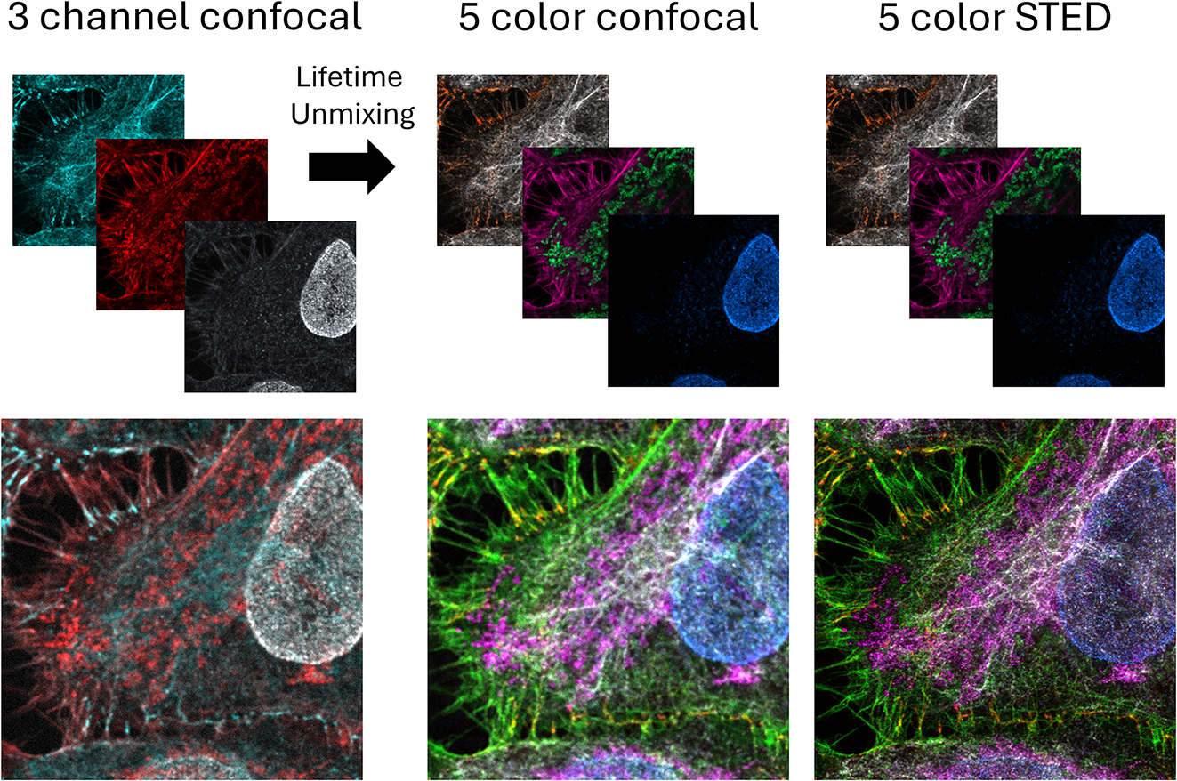
Summary showing how 5-color confocal and STED images were generated from 3 fluorescent channels with lifetime information. From each of the first two confocal channels, two lifetime images were extracted (not shown). Those grayscale images, each representing one fluorochrome, were pseudocolored with different hues, here orange (WGA CF594) and white (antibody detection of vimentin with Alexa Fluor Plus 594) or magenta (actin detected with phalloidin ATTO647N) and green (antibody detection of mitochondria with Abberior Star 635P). The third confocal channel (antibody detection of nuclear pores with CF670R) was cleared up from spectral bleed-through and noise using lifetime features to produce the image of the fifth fluorochrome (blue). The five images were then overlaid (bottom). The same procedure was applied to STED images, the 3 channel STED images are not shown.
2 Materials and methods
2.1 Sample preparation
Fixation methods and staining protocols do not differ from normal immunostaining procedures and therefore are not described in detail.
2.1.1 Labelling
We performed antibody labeling of HeLa cells grown on coverslips with primary and secondary antibodies. With many targets this quickly gets complicated because most available primary antibodies are from rabbit or mouse and thus may limit the number of detectable antigens. Fluorescence labeling of primary antibodies by either fluorochrome conjugation or via preincubation with fluorochrome labeled nanobodies or similar approaches may alleviate this problem but we did not test this approach for lifetime color separation. Fluorochrome labeling of primary antibodies may result in weaker signals since no amplification by a second layer takes place. Other staining methods such as fluorescence in situ hybridization (FISH) should also work, but again we have no experience with this.
For lifetime separation, we found that we can cleanly separate two fluorochromes per channel from each other, but not more [45], see Section 3.2 for detailed discussion. We were successful with the fluorochromes as listed in Table 1 in a five color sample (Figure 1). While the highest available excitation wavelength in our systems, 670 nm, that we used for CF680R also excites the dyes in the far-red channel (ATTO647N and AS635P), the lifetime of CF680R was short enough, so that it could be separated from the other fluorochromes by lifetime [40] (Figures 7 and 9). Staining with WGA-CF594 (10 min; Biotium, 29023-1) was performed on live cells to limit the staining to the cell surface. Otherwise WGA also labels additional glycosylated proteins such as internal membrane proteins and nuclear pores. WGA sometimes redistributes during further steps, giving generally variable staining results. Fixation was for 10 min in 4 % formaldehyde in PBS. Air drying was carefully avoided at all times to preserve structural integrity. Postfixation with 1 % formaldehyde in PBS for 10 min was performed to minimize diffusion of fluorochromes in the sample [40]. Five color sample, primary antibodies: Chicken IgY anti-vimentin polyclonal (Invitrogen, PA1-10003, diluted 1:1,000 in Blocking solution); Rabbit anti-TOMM20 polyclonal (Sigma, HPA011562, 1:200); Mouse anti-NUP107 monoclonal (39C7) (Invitrogen, MA1-10031, 1:100). Fluorochrome coupled secondary antibodies: Goat anti-chicken IgY (H + L) cross-adsorbed, Alexa Fluor Plus 594, polyclonal, (Invitrogen Thermo Fisher A32759, 1:500–1:1,000); Goat anti-rabbit Abberior STAR 635P, polyclonal (Abberior, 2-0012-007-2, 1:200); Donkey anti-mouse IgG CF680R, polyclonal (Sigma-Aldrich, SAB4600207, 1:200). Staining with phalloidin ATTO647N conjugate (ATTO-TEC, AD 647N-81, 1:2,000) was after the secondary antibody. For further details see [40].
Fluorochromes and what they were attached to in the five color sample.
| Channel | Label 1 | Label 2 |
|---|---|---|
| Near red | CF594-wheat germ agglutinin | Alexa Fluor Plus 594 goat-anti-chicken antibody |
| Far red | Abberior Star 635P goat-anti-rabbit antibody | ATTO-647N – Phalloidin |
| 670 nm exc | CF680R-donkey-anti-mouse antibody |
In confocal images Alexa Fluor Plus 647 could be well separated from ATTO647N (Figure 4) or Abberior Star 635P, but in STED it bleached fast. For the two-color sample, phalloidin-ATTO647N and the primary anti-TOMM20 antibody were as above, the latter was detected with a polyclonal Alexa Fluor 647 Plus-labeled goat-anti-rabbit antibody (Invitrogen Thermo Fisher, A32733).
2.1.2 Good samples for microscopy
The mounting medium plays an important role in the optical path: most mounting media for slide-coverslip samples have a refraction index lower than coverslip glass. Therefore, spherical aberration is introduced into the optical path. With increasing distance from the coverslip this has an increasing negative impact not only on resolution but also on fluorescence intensity since the produced fluorescence photons are smeared over a larger volume rather than kept in a tight and therefore bright point spread function [46]. Therefore, wherever possible, the object of interest should be sitting on the cover slip and not on the glass slide.
Our samples were mounted in Fluoromount G (Invitrogen, 00-4958-02). This mounting medium does not harden and thus avoids shrinkage of the sample, an effect that is counterproductive for high resolution microscopy. We seal the samples around the edge of the coverslip with transparent nail polish.
The thickness of the coverslip should be 0.17 mm, as indicated on the barrel of most objectives. This is the thickness for which the optical correction of the objective is calculated. Deviations also cause spherical aberrations. Unfortunately, most coverslips are thinner than that. The widely spread “number 1” or “#1” thickness is 0.14–0.17 mm and thus usually too thin. Better options are #1.5 (0.16–0.18 mm) and #1.5H (0.165–0.175 mm). Hecht-Assistent, Marienfeld and others provide such coverslips.
2.1.3 The actual lifetimes of fluorochromes in a sample
The lifetimes of fluorochromes depend on their chemical structure but also on their environment. Some companies now provide the lifetime of their fluorochromes free in solution. This is an improvement but still merely a rough indicator what the lifetime will be in the final sample. The same fluorochrome can have different lifetimes depending on the binding partner such as antibodies or other molecules [26], [41]. A striking example are the lifetimes of ATTO647N and Abberior Star635P when bound to either antibodies or phalloidin, a molecule that binds to actin fibers. For both dyes, the lifetime changes with the binding partner so strongly that we could successfully separate the actin signal from the antibody target by lifetime, although only a single fluorochrome was used [40]. Lifetime is likely to be different in different mounting media. It also varies somewhat in repeated, similar lab experiments. In essence, the lifetime and the difference in lifetime for a given pair of fluorochromes to be separated in a given spectral channel must be confirmed under actual sample conditions.
2.1.4 Conditions for successful lifetime unmixing
We found that for separation by lifetime, a lifetime difference of 0.8 ns between two dyes (measured by confocal microscopy under actual sample conditions, see previous section) is sufficient for both, confocal and STED microscopy. With a difference of 0.8 ns separation typically works well even if the labeled targets show close proximity in space. In STED images, due to application of the STED beam the lifetime of a fluorochrome is significantly shortened. (The position in the phasor diagram shifts in direction of the lower right corner, see Section 2.3.1, Figures 2 and 3, compare Figure 6A and B). This means that for two dyes also the actual difference between the lifetimes is shorter than in confocal images. Therefore, in STED the required difference in lifetime measured by confocal FLIM is bigger than for separation in confocal images. Thus, for confocal microscopy differences smaller than 0.8 ns should be sufficient for successful separation, but we did not explore the limit. Since the actual lifetime in STED varies with the power of the depletion beam, no reasonable value can be given for a “Lifetime in STED”. All lifetime values given in this article were measured in the confocal mode.

Schematic drawing showing the relationship between the intensity grayscale image (left), the FLIM image (center) and the phasor plot (right). With a lifetime capable microscope, in addition to the intensity image, the lifetime image can be recorded, where every pixel has an average lifetime value. From these values a phasor can be created. Pixels with similar long lifetimes (pink), similar intermediate lifetimes (green), and similar short lifetimes (blue) will form clusters on the phasor plot.
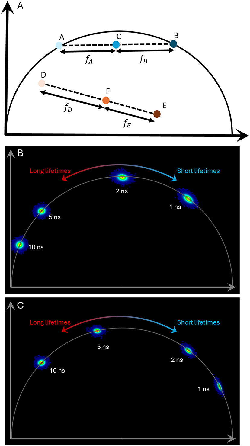
Phasor, behind the scenes. (A) Points A-C-B show the situation with two fluorochromes with different lifetimes, both with single exponential decay (points A and B). Pixels containing both fluorochromes will be positioned on the line between points A and B, for example at C. The length of fA and fB is directly related to the ratio of the two fluorochromes in the respective pixel. D-F-E show the respective situation when the two fluorochromes do not have a monoexponential decay. (B) Phasor plot with multiple monoexponential lifetimes (simulated data). Monoexponential lifetimes are located on the universal circle (semi-circle), with short lifetimes towards the right and long lifetimes towards the origin (left bottom corner). Multi-exponential lifetimes are located inside the circle. The scaling of lifetimes is not linear and depends on the repetition rate of the laser. This plot reflects the situation with 80 MHz repetition. The same distribution is achieved with 40 MHz and a harmonic setting of 2 (compare Figure 4E and F). (C) As in B, but with a repetition rate of 40 MHz (and no increase of the harmonic).
2.2 Image recording
2.2.1 Microscopes
The imaging procedures in this protocol were established on two Leica Microsystems TCS SP8 WLL FALCON systems with linear scanning mode. These systems perform time-correlated single-photon counting (TCSPC) to determine fluorescence lifetimes. One, a mixed confocal and multi-photon setup, is based on an upright DM8. The other SP8 is based on an inverted DMi8 stand and has STED super resolution capabilities with a pulsed 775 nm depletion laser. We expect our fluorochrome separation approach to work with FLIM systems from other manufacturers as well but we did not have the opportunity to test it.
Our two systems have the following characteristics: A pulsed white light laser (WLL) allows to pick any wavelength between 470 and 670 nm for one-photon excitation. 80 MHz repetition rate with 200 ps pulse width. In confocal mode the repetition rate can be reduced to 40 or 20 MHz if desired. In STED mode the repetition rate is slaved to the 80 MHz of the depletion laser. Detection windows are spectrally freely definable with 1 nm steps due to the detectors being behind a prism. Single molecule detection hybrid photodetectors (“SMD-HyDs”) allow high single photon count rates due to short dead times. FLIM is also possible with “normal” HyDs, but SMD-HyDs are selected for low noise and allow higher count rates (1 count per pulse as opposed to 0.5 per pulse), according to the manufacturer. On the STED system, the STED donut originates from a 775 nm 80 MHz Laser with 650 ps pulse width. NA 1.4 Plan Apo oil immersion objectives were used, a 63× on the upright system and a 100× “STED white” objective on the STED system.
2.2.2 Imaging parameters for confocal and STED
2.2.2.1 Sequential recording and image settings
The two-color sample with Alexa Fluor 647 Plus and ATTO647N was recorded with excitation of 0.5 % laser power at 633 nm (≈3 μW at the sample plane), emission window 650–800 nm with two detectors in tandem at 650–668 nm and 668–800 nm. Two detectors in tandem allow to record twice as many photons per second without saturation compared to a single detector. Lower excitation power and a single detector would have worked but would have taken longer. Data from both detectors were combined to obtain a single intensity and FLIM image. We used a scan speed of 200 Hz (lines per second) and set the frame accumulation to 50 to obtain optimal image contrast, although fluorochrome separation is already possible with a single frame (Figure 4).
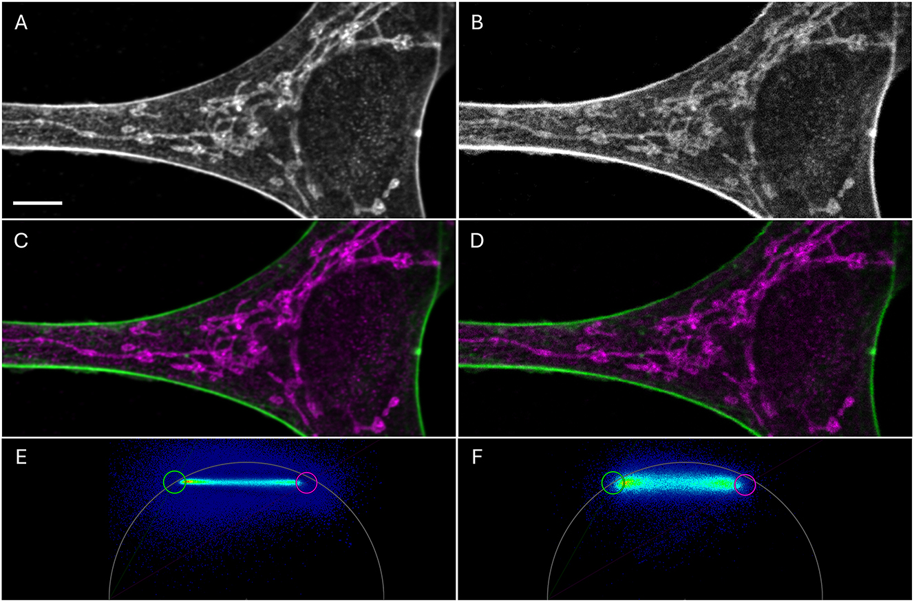
Confocal images of a cell labeled with ATTO647N-phalloidin (actin skeleton, green, lifetime 3.1 ns) and Alexa 647 Plus TOMM20 (mitochondria; magenta, lifetime 2.0 ns). The images were generated from 50 accumulated frames (A, C, E) or with just one frame (B, D, F). Note the signal to noise difference. (A–B) Intensity image with an average number of photons in the bright actin filaments of 7,500 in A and 120 in B and in the dimmer mitochondrial signals 2,500 in A, 60 in B. Scale bar 5 µm. (C–D) Actin and mitochondrial signals were separated in two grayscale images, false color coded and overlaid. (E–F) Phasor plot used for the color separation of C and D, respectively. Repetition rate was 40 MHz and the harmonic was set to 2, so the phasor plot appears like an 80 MHz phasor plot. Threshold values (see main text) were 100 and 1 photons, respectively. For circles see main text and next figure.
When selecting excitation wavelengths for neighboring channels care should be taken that a wavelength with a high excitation of the desired fluorochromes but a low excitation of spectrally neighboring fluorochromes is selected. For the five color confocal and STED sample (Figures 1, 6, and 7), three frame-sequential sequences were recorded to minimize spectral crosstalk in the following order (775 nm depletion only in STED mode):
exc. 5 % at 670 nm (≈17 µW)/em. 700–750 nm/775 nm STED at 5 % (≈17 mW)
exc. 6 % at 633 nm (≈28 µW)/em. 640–680 nm/775 nm STED at 20 % (≈68 mW)
exc. 3 % at 594 nm (≈12 µW)/em. 600–630 nm/775 nm STED at 30 % (≈102 mW)
The sequences move from longest to shortest excitation wavelength to minimize bleaching. Particularly for STED recordings where the 775 nm depletion causes some anti-stokes excitation of the longer wavelength dyes this is important. If available use notch filters for every excitation and STED laser wavelength to minimize the contribution of reflection. Before recording, the fully integrated FLIM module must be started within the Leica software so that not only the intensity image but also the lifetime information is recorded.
For the examples above, we used a scan speed of 400 Hz (lines per second) for the five-color sample and 200 Hz for the two-color sample. With the respective software control, we set frame accumulation for confocal FLIM images to 20.
2.2.2.2 More frames for STED images
In STED we increased frame accumulation to 100. For truly point-like signals, both STED and confocal imaging should result in the same signal intensity (number of photons) when the beams are centered on the structure, because all of the signal originates from a point that is in the center of the STED donut anyway. For signals from extended structures such as fibers, however, depletion will reduce the signal intensity, because signal from neighboring parts of the structure is suppressed, the detection volume is smaller.
Other influences are introduced by the scanning process: In STED, pixels sizes are typically smaller, in our case linearly about 3× smaller. (∼25 nm, compared to ∼75 nm in confocal). If all other settings are kept the same this results in a ∼3× shorter pixel dwell time and thus 3× less photons per pixel. On the other hand, the scan lines are 3× closer together so that light from a given structure is recorded more often and thus additional photons are collected.
In practice, we observe that more frame accumulation is required in FLIM-STED compared to confocal images to detect a reasonable number of photons in pixels with signals.
2.2.2.3 Further parameters for a STED recording
To record STED images we typically apply the following additional parameters: Pinhole at 0.93 AU@580 nm. This helps to increase the Signal to Background ratio. Optimized pulse delay between the WLL and STED depletion laser was determined to be at 200 ps in our system. The correct delay timing is important to maximize the STED effect: If the depletion pulse comes too early it has no effect, if it comes too late, many photons are already emitted before depletion can occur. In both cases total signal will be brighter than in the optimal scenario. Hence, the timing can be optimized for lowest intensity = strongest depletion. Pixel size was 21–26 nm. Image size will depend on zoom factor and number of pixels used.
With these parameters, recording of a STED image with 1,552 × 1,552 pixels and all three sequences with 100 accumulations each takes about 13 min.
2.2.2.4 Pulse rate in confocal images
For confocal imaging, the pulse rate can be reduced from 80 to 40 or 20 MHz. 80 MHz translate into one pulse every 12.5 ns. For fluorochromes with average lifetimes of several nanoseconds, a rather small but noticeable fraction of photons will thus be detected only after the next pulse (in the next cycle) and thus result in a measured lifetime that is slightly shorter than the actual lifetime. However, for separation purposes the exact measured lifetimes do not matter, the lifetimes of different fluorochromes just have to be different enough.
Reduced pulse rates also result in respectively less collected photons per second, increasing overall imaging time to reach the same image quality. For fluorochrome separation by lifetime, 40 or 80 MHz pulse rates deliver good results for many samples.
2.3 Image analysis: lifetime unmixing via phasor for confocal and STED images
2.3.1 Background: the phasor of lifetime images
A phasor diagram is a graphical representation of the lifetimes found in a given image in a polar plot, based on the sine-cosine transforms of frequency domain information. Thus, the phasor is also called “polar plot” by some authors [47], [48]. TCSPC provides time domain information however, so that a Fourier transformation is performed to obtain the frequency domain data. A description of phasors in FLIM and how they are mathematically generated can be found in Ref. [39]. In the following we explain how a phasor represents the FLIM image as a foundation for the lifetime separation in the next section.
In this section, the term “pixel” always refers to a pixel in the confocal or STED image (and not the phasor plot image). Each pixel is represented by a single dot in the phasor plot, positioned according to the average lifetimes of the present fluorochromes (Figures 2 and 3B, C). Lifetime is an intrinsic characteristic of every fluorochrome in a given environment, leading to a specific phasor pattern. In phasors from microscopic images, many pixels will be represented in neighboring positions in the phasor plot since they have similar lifetime components (Figure 4E and F). Areas in the plot where dots lie on top of each other are color coded. In our plots (from the Leica LAS X software) a rainbow color code with blue for low occurrence to red for high accumulation of dots is used.
For an image with two fluorochromes with different lifetimes a phasor plot will show three scenarios: pixels containing only the longer lifetime dye (region A or D in Figure 3A). Pixels containing only the shorter lifetime dye (Region B or E). And pixels containing a mixture of both (region C or F). Phasor plot locations of pixels containing only one dye will correspond to the location obtained with single stained samples. Pixels with a mixture of both dyes will be located along a line between the positions of the individual dyes. This is where the “linear property” of the phasor is powerful: The exact position of the pixel in the phasor is defined by the fraction of the components of the two dyes (Figure 3A, fA, and fB). Hence, from the position of the pixel in the phasor diagram, the percentages of its photons belonging to dye A and dye B can be extracted.
An advantage of the phasor plot is that, as opposed to curve fitting, for its generation there is no need to choose parameters from a range of possibilities such as the number of expected lifetime species. The phasor diagram is based only on mathematical calculations, no fitting is required: The same data will always generate the same phasor plot. Avoiding the fitting procedure which requires user input makes the technique more robust. Thus the phasor is a powerful tool for lifetime analysis with its robustness and ease of use among its biggest advantages.
2.3.2 Separation of fluorochromes by phasor analysis
Image analysis was performed with Leica LAS X software version 4.1.1.23273 which we installed on a separate computer. This is not the version that comes with the SP8 (LAS X 3.X) but the variant for the SP8 successor “Stellaris”. It contains an extended, user friendly suite of tools for phasor lifetime analysis. A “separate”-button makes unmixing procedures easier, compared to the 3.X version. We have trained users without previous FLIM experience and they became quickly autonomous for their lifetime analysis. LAS-X 4 installation files were kindly provided by Leica Microsystems CMS. License dongles appear to be compatible between the 3.X and 4.X versions.
2.3.2.1 Parameters
To achieve an acceptable phasor unmixing, as a rule of thumb at least 100 photons per pixel should be collected in those regions that contain fluorescence signal (Figure 4B and D). One can obtain results with dimmer images, but results may vary depending on other parameters, such as background and overlap between labelled structures.
An unfiltered phasor plot is generated using every pixel in the image: Pixels with only a few photons of background noise are also displayed and may confuse the clarity of the data presentation. They can be suppressed by estimating the background intensity (in number of photons) and entering this number as threshold in the software. Pixels with a photon number below threshold will then not be displayed in the phasor. This is recommended. In LAS X, there is a threshold menu in the phasor menu. The highest value that can be entered is 100 photons, typically we apply around 20–50.
STED images, including FLIM-STED images, typically have low photon numbers per pixel, leading to unfavorable signal-to-noise ratios that can impede the extraction of information from phasor data. To enhance data visualization and improve analysis and interpretation, filters can be applied to the image before calculating the phasor. Traditionally, median filters have been used in phasor analysis to tackle this issue. However, median filters degrade high spatial frequency FLIM information, particularly affecting edges of features, puncta, or any fine structures. We recommend using a wavelet filter instead, if available. Wavelet filtering preserves said features and is thus beneficial when working with low photon numbers [49].
The lifetime distribution and dynamic range of the phasor depends on the repetition rate of the pulsed laser used. The higher the repetition rate, the further to the left the positions for given lifetimes will move. Ideally, the lifetimes of a given image should be in the central range of the phasor because then the distance between different lifetimes will be largest. For lifetimes between 1 and 4 ns a repetition rate of 40 MHz or 80 MHz is well suitable (Figures 3B, C and 4E, F).
If for some reason an image has to be recorded with a rather low repetition rate, the phasor can be adjusted by applying a harmonic value of 2 or higher (see legend to Figure 4B). In a Fourier Transform, a periodic waveform can be decomposed into a series of sinusoidal waves. The fundamental frequency is the lowest frequency of the waveform, and the harmonics are the higher frequencies that are integer multiples of this fundamental frequency. Adjusting the harmonic number alters the harmonic wave that the respective lifetime is multiplied by. For very short lifetimes, the regions of interest on the phasor plot are situated in the lower right corner (blue in Figure 2). By increasing the harmonic number the visualization of these regions is expanded and shifted closer to the middle of the universal circle (Figure 3B and C). This results in a more convenient visualization of the data, with larger distances between the values. For more details see [39].
2.3.2.2 Separation of two fluorochromes by lifetime
Figure 4 shows a cell where the actin skeleton (green) and mitochondria (magenta) were labeled with dyes with similar spectral properties but different lifetimes. In the intensity image (A, B) the two fluorochromes cannot be distinguished, but a good separation by lifetime was achieved (C, D). The phasors are shown in E, F.
Using the tools provided in the Leica software, areas identified to contain the pattern of single dyes were selected in the phasor plot (Figure 5), and a linear separation was conducted (see Figure 5 legend for details). The software makes use of the linear property of the phasor plot. The algorithm takes the centers of two circles (Figures 4E, F and 5) which are defined by clicking on the phasor plot as the single dye references for the separation. The centers of the circles define the maximal and minimal lifetimes for the separation. Having them positioned outside the actual distribution makes sure that no signal pixel is outside the defined range of lifetimes thus “saturation” does not occur. The radius of the circles has no effect on the analysis. Figure 5 shows a screenshot of the software’s user interface. Results are shown in Figure 4C and D and for a different sample in Figure 6.
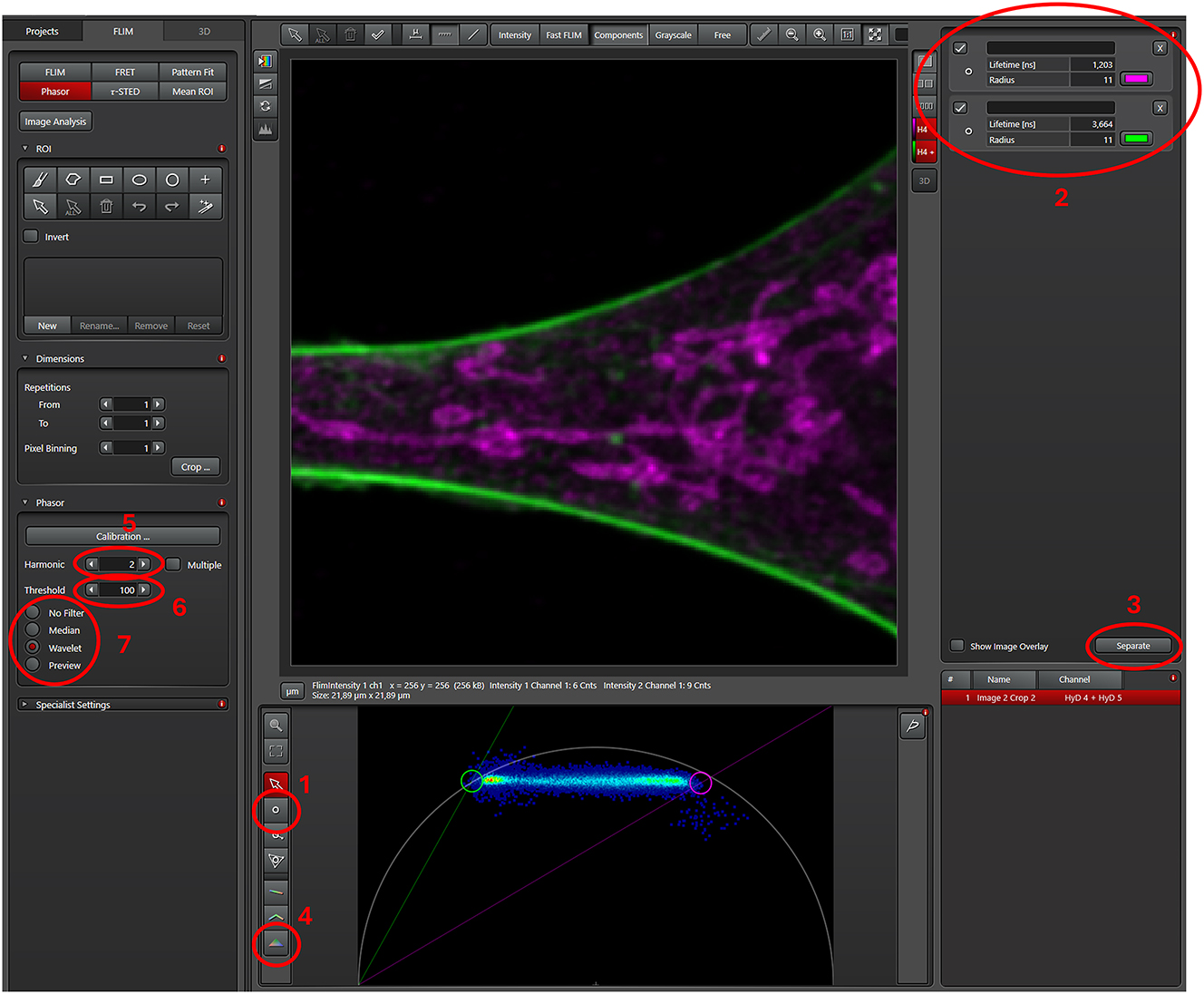
User interface of the FLIM window of the LAS X software. Only a part of the cell from the previous figure is shown and represented in the phasor. Using the “draw cursor” tool (ROI 1), two areas slightly outside of phasor signature of the single dye lifetimes are marked (circles). Depending on the labelling intensities, the locations can be either seen clearly (like here) or not. Single color references can be used as control to determine the phasor signature of said dye for later use. The lifetime of the two circle-cursors and the assigned pseudocolors are displayed at the top right corner (ROI 2). When satisfied with all settings, a click on the separate button (ROI 3) starts the phasor based unmixing. The final two unmixed images are displayed. Once the images are saved, they can be exported as 16-bit tiff files. The triangle tool for more complex unmixing (see Figures 7 and 9) is below the “draw cursor” tool (ROI 4). The harmonic, threshold and phasor filter can be changed as needed on the left (ROI 5, 6 and 7, respectively).
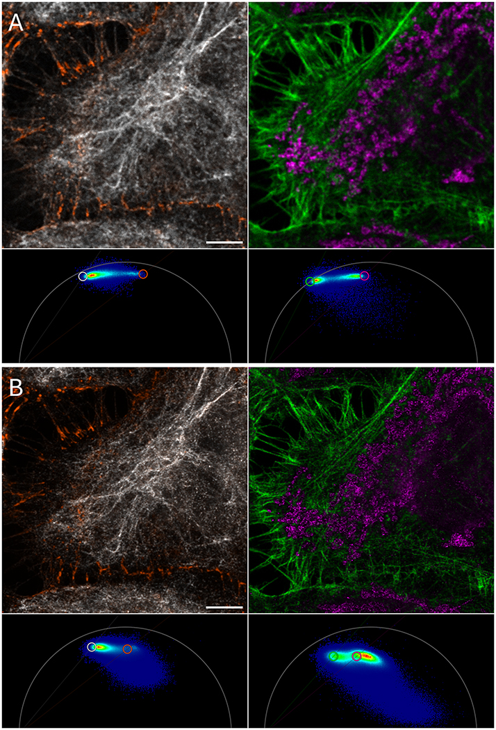
Five-color sample, unmixing of sequences with two fluorochromes, based on the displayed phasor plot. (A) Confocal images. (B) STED images. Left: vimentin in white (Alexa Fluor 594, lifetime 2.6 ns) and WGA in orange (CF594, 1.7 ns). Right: phallodin labeled actin fibers green (ATTO647N, 3.5 ns) and mitochondria in magenta (Aberrior Star 635P, 2.0 ns). In the STED phasor plots, due to the stimulated depletion, the photophysics is more complex than usual. Hence the different positioning of the cursors in STED phasors. In STED phasors, the “top left” fraction of each fluorochrome’s signature contain the most informative pixels (see main text and Figure 8) and the curser is set to represent those. This different positioning is only applicable to STED phasors. Confocal images were separated as described above. Scale bar 5 µm.
Separated images were saved and exported. Pseudocoloring and overlay to obtain final images as in Figure 1 bottom was performed in a different software, Fiji or Imaris.
2.3.2.3 Removing bleed-through, autofluorescence and reflected photons
The phasor can also be used to filter non-desirable contributions from spectral bleed-through or autofluorescence. In Figure 7A, ATTO647N–Phalloidin bleeds through to the CF680R channel: Actin fibers are dim but clearly recognizable, e.g. in the top left quadrant of this confocal image. The ATTO647N label was quite strong and still somewhat excited at 670 nm which was used for CF680R. Excitation with 680 nm would be more suitable [40] but was not available on the SP8 systems. Since no notch filter was available to suppress reflection of 670 nm, the recorded image also contained considerable amounts of reflected photons with 0 ns lifetime. Pixels containing only reflected photons are represented at the lower right corner of the phasor plot (Figure 7C). However, most of them are below the set threshold value (see above). Note that compared to Figures 4 and 5 the ATTO647N distribution is elongated in the phasor, towards the bottom right corner. The intensity of this bleed-through signal is close to background levels. The respective pixels thus contain a considerable percentage of reflected photons, hence the elongation towards the bottom right corner.
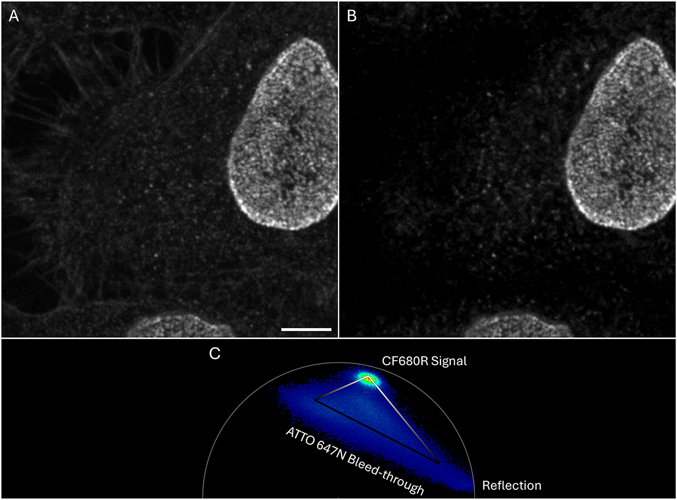
Confocal images of cells with labeled nuclear pores (CF680R-NUP107; lifetime 1.5 ns) and bleed-through from ATTO647N-phalloidin (3.5 ns). Only the CF680R-channel of the 5-color sample is shown. Filtering of the ATTO647N and reflection is performed with the phasor. (A) Raw intensity image where the actin filaments can clearly be seen (ATTO647N bleed-through). (B) Filtered image where the ATTO647N contribution is eliminated. (C) Phasor used to generate the filtered image. See Figure 9 for explanation of the triangle. Scale bar 5 µm.
Lifetimes of ATTO 647N (3.5 ns) and CF680R (1.5 ns) were sufficiently different from each other and from the reflected photons (0 ns) to separate them (Figure 7B). Image filtering was done using a tool in the shape of a triangle (Figure 7C; see Figure 5, ROI 4 for tool location in the software). The triangle tool is suitable if three components are present from which only one is to be kept. This tool uses a lifetime gradient based on the phasor coordinates and assigns an intensity value to the pixels depending on their position on the phasor, hence to their lifetime (see Figure 9 for detailed explanation).
2.4 Image analysis: Tau-STED and STED-anti-stokes excitation
Resolution in STED images can be improved by lifetime approaches such as “gated STED” which during acquisition discards all photons with very short lifetimes, e.g. <0.5 ns, since this “gate” contains fluorescence photons emitted before depletion took effect as well as reflected photons [50]. SPLIT-STED is another example. It uses fluorophore lifetime dynamics under CW-STED conditions (depletion with continuous wave laser) to effectively differentiate photons emitted from the central region (not affected by depletion) and from the outer edges of the excitation (affected by depletion) [51].
In contrast to gated STED, a fully lifetime capable system can use lifetime also post acquisition to improve the resolution and achieve the best possible result. The depletion laser modifies the photo dynamics of the population of fluorophores that it affects, including their average lifetime. The lifetime modification depends on the local depletion light intensity. Since the STED doughnut is a Gaussian beam, its intensity is uneven across the PSF. This leads to variable average lifetimes, depending on the exact position of the fluorophores (Figure 8). This displaced, elongated distribution of average lifetimes (compared to confocal) can be seen and characterized in the phasor (compare Figure 6A and B, compare Figures 7C with 9C).
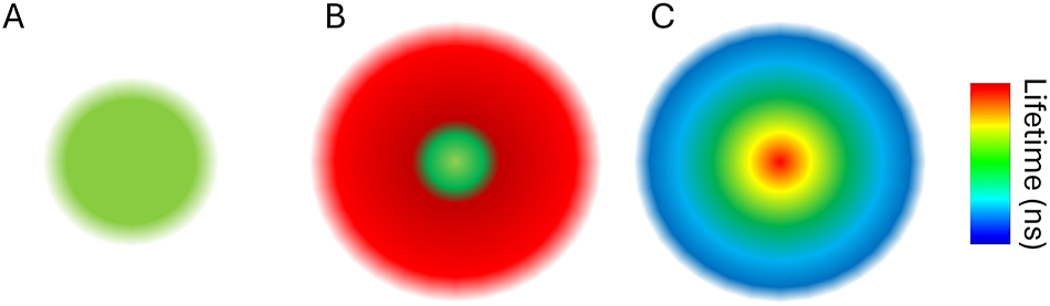
Lifetime in STED. (A) Scheme of the Gaussian excitation. (B) STED depletion profile (red) over the excitation leads to a smaller sampling volume. (C) Schematic representation of the lifetime distribution across the STED point spread function. The fluorescence lifetime is shortened more where the depletion is stronger. In the center, the fluorescence lifetime is the same as in the absence of STED.
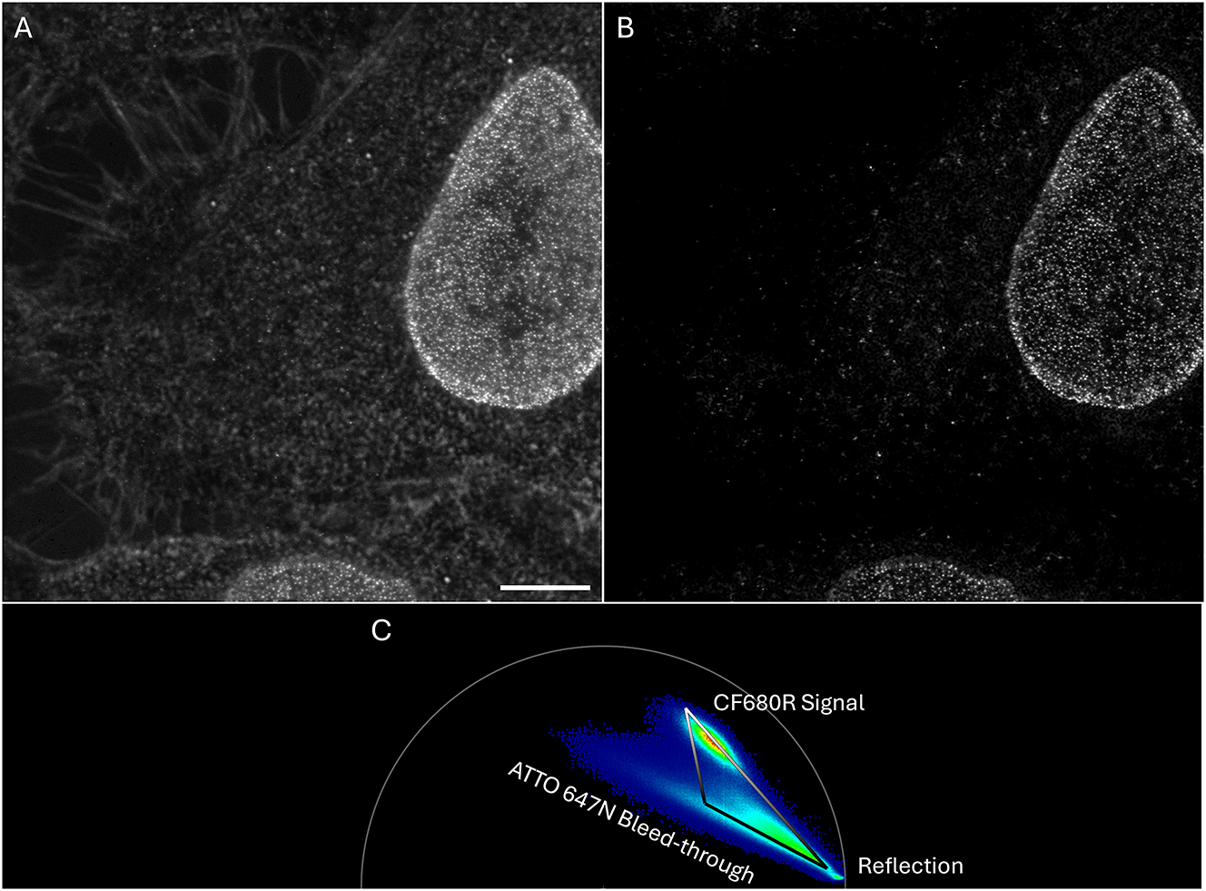
τSTED example. Fluorochromes and labels as in Figure 7 but note the improved spatial resolution. (A) Raw STED image. (B) τSTED corrected image. (C) Phasor plot of image (A) used for the τSTED correction shown in (B). The various contributions to the phasor plot can be easily identified. The top part of the right edge of the triangle represents the pixels with the desired CF680R signals. Pixels at the top corner of the triangle have 100 % intensity (meaning intensity in the final image (B) is the same as in the original image (A)). In current τSTED-phasors, the two lower corners of the triangle always represent zeros, meaning pixels at those corners and on the line between them (zero line) are black in (B). For all other pixels, the intensity in the final image (B) (between 0 and 100 % of the intensity in (A)) is linearly dependent on the distance to the triangle’s top corner and to the zero line (compare Figure 3A). Scale bar 5 µm.
τSTED (“Tau-STED”) is a name Leica gave to a proprietary algorithm that applies background correction and filtering of pixels based on their phasor signature [52]. The current version works best if a spectral channel contains one desired fluorochrome. A vector can be drawn in the phasor plot (right edge of triangle in Figure 9C) to separate pixels with photons mostly unaffected by the depletion process (longer lifetimes) from pixels with many depletion affected photons (shorter lifetimes, compare Figure 8C). In addition, those pixels that do not correlate with the drawn vector can be identified as containing noise and filtered out (see legend to Figure 9). This approach addresses issues of reflection, low-resolution photons (short lifetimes), and crosstalk (different behavior of different dyes) commonly seen in STED multicolor experiments. The accuracy of this determination, as with all lifetime-based approaches, depends on the available photon budget.
For the spectral channel in our five color STED images containing the CF680R antibody staining of nuclear pores, the τSTED function in LAS X was used (Figure 10). After activating Expert mode (see Figure 10) the phasor appears in the bottom right corner of the user interface. With the “Draw color coding triangle” tool (ROI 2 bottom) a triangle was placed on the phasor (Figures 9C and 10) and the τSTED image was generated (Figure 9B).
![Figure 10:
User interface of the τSTED part of the LAS X software. The expert mode shown here is needed only for complex samples (see main text) and activated at ROI 1. Else the τ-STED-mode can be used. As explained at Figure 5, either a line or a triangle tool (ROI 2) can be used for lifetime filtering. Here the triangle tool was applied to filter out ATTO647N bleed-through, noise and reflections (see Figure 9 and main text). Different parameters for the strength of the filtering are in ROI 3. Typically, they can be left at the default values. With increased τ-Strength values, more weight is given to long-lifetime signals. The physical limit is set by the photon budget and signal-to-noise ratio. See [52] for further information. Once the τSTED image is generated it should be saved by clicking “Save image” on the bottom left corner of the FLIM window (surrounding the window shown here) or by right click on the image. It can be exported as 16-bit tiff file.](/document/doi/10.1515/mim-2024-0022/asset/graphic/j_mim-2024-0022_fig_010.jpg)
User interface of the τSTED part of the LAS X software. The expert mode shown here is needed only for complex samples (see main text) and activated at ROI 1. Else the τ-STED-mode can be used. As explained at Figure 5, either a line or a triangle tool (ROI 2) can be used for lifetime filtering. Here the triangle tool was applied to filter out ATTO647N bleed-through, noise and reflections (see Figure 9 and main text). Different parameters for the strength of the filtering are in ROI 3. Typically, they can be left at the default values. With increased τ-Strength values, more weight is given to long-lifetime signals. The physical limit is set by the photon budget and signal-to-noise ratio. See [52] for further information. Once the τSTED image is generated it should be saved by clicking “Save image” on the bottom left corner of the FLIM window (surrounding the window shown here) or by right click on the image. It can be exported as 16-bit tiff file.
The triangle tool (and not the line tool) was used because in this particular case the strong ATTO 647N Phalloidin staining in the neighboring spectral channel caused crosstalk into the CF680R channel. However, ATTO 647N and CF680R have different lifetimes. ATTO 647N is distributed in a very elongated cluster, since this bleed-through signal is weak and close to the background level (see above). Thanks to the lifetime difference, the phasor signatures of theses dyes are in different positions on the phasor plot. Reflection and low resolution photons were also filtered out to obtain a crosstalk and background corrected image (Figure 9B). See legend to Figure 9 for details.
In the case shown here, expert mode was used because of the complexity of the sample. For a spectral channel with only a single fluorochrome with minimal bleed-through, the “τSTED” mode (ROI 1, center), is sufficient. In this mode, the software predicts what would be the best trajectory, and applies it automatically.
The generated image should be saved before export.
3 Results and discussion
3.1 Phasor based separation by lifetime
We demonstrated that two fluorochromes per spectral channel can be separated in confocal (Figures 4 and 6A) and STED microscopy (Figure 6B) if their lifetime is sufficiently different. Exploiting this, we generated multi-color confocal and FLIM-STED images with five colors from only three spectral channels (Figure 1). In our previous publication we demonstrated that the remaining bleed-through between lifetime separated images is well in the range of spectrally separated images [40]. Lifetime separated images can thus have the same quality as spectrally separated images. Others have shown that phasor based separation is also possible in image-scanning microscopy [42] (ISM), an approach were the confocal pinhole is replaced with an array detector to avoid loss of light while obtaining optimal confocal resolution [53].
Color separation by phasor analysis is feasible with much smaller numbers of photons (Figure 4B, D, and F) than separation by curve fitting, because the phasor is more accurate to calculate the average lifetime of multi-exponential decays with low photon counts and SNR [48]. With curve fitting, two fluorochromes with multiexponential decay would further increase the complexity with their additional exponential components. For more components more photons are needed for an accurate fit. Hence phasor analysis is superior for lifetime unmixing with small photon numbers.
We would like to point out that all procedures were performed with commercially available fluorochrome-coupled antibodies or other reagents, commercial hardware and software. We have the hope that the above detailed protocols will help to motivate others to use these procedures in their own multi-color fluorescence experiments.
3.2 Separating more than two fluorochromes by lifetime?
The procedure described above works well with spectral channels containing two fluorochromes with different lifetimes (Figures 4 and 6). An obvious question is whether more than two fluorochromes can be separated by lifetimes. We tried this with Abberior STAR 635P on antibodies, Alexa Fluor Plus 647 labeled antibodies and ATTO 647N-Phalloidin (lifetimes of 2.0, 1.2, and 3.5 ns) [40]. While any two of this set could be separated, separation of all three, while possible, resulted in loss of detail and thus suboptimal image quality. The technical problem that arose was that the lifetime position of the three fluorochromes in the phasor plot more or less formed a line. Any pixel in the middle of the line could correspond to either a mixture of the dyes with the longest and the shortest lifetime, or a significant contribution of the dye with the intermediate lifetime. Under such conditions, a good separation only would be possible if the fluorochromes would label spatially separated and identifiable structures such as nuclear speckles versus cell membranes. But then also a single fluorochrome would do.
Successful separation of three fluorescent species based on the phasor plot was reported by others, however [41], [54]. In these cases the positions of the three fluorescent species formed a triangle in the phasor plot. Thus, a unique solution could be identified for each phasor position. In one case lifetimes were 3.71, 3.05 and 2.14 ns, with the 2.14 ns lifetime coming from a tri-exponential decay and thus a position away from the universal circle so that the three phasor positions indeed formed a triangle despite the small lifetime differences [41]. While generally good separation was shown, close inspection of pictures with overlapping structures (e.g. their Fig. S31D) reveal some separation artifacts though. Qdot 585 (longest lifetime), Bodipy TMR (intermediate lifetime), and AF555 (shortest lifetime; in other reports this dye is called Alexa Fluor 555 or Alexa 555), all coupled to antibodies were also successfully separated [54]. The actual lifetimes were not given in this report, but other publications give around 0.7 ns for antibody bound AF555 [26] and 19.5 ns for free Qdot 585 [55].
A separation of four fluorochromes using the phasor plot was also reported [56]. Transformation of the phasor plot to higher harmonics (Figure 3B and C) resulted in additional equations so that a unique solution for four components could be determined. Respective lifetimes covered a wide range: 12, 3.8, 1.4 and 0.6 ns. Since currently commercially available labels on antibodies do not exceed 5 ns (to our knowledge), it currently may be difficult to perform this approach with immunostained samples.
3.3 Conclusion: recommendations for multi-color fluorescence
It currently seems easiest to first explore the possibilities of spectral separation of a given instrument, in particular since spectral separation is broadly available. We successfully used six spectrally different colors on our confocal SP8 systems, five excited with the white light laser (470–670 nm) plus DAPI excited with 405 nm. New systems may allow even more spectrally separable fluorochromes. For projects where the spectral options are exhausted, either because more fluorochromes are needed or because of special constrains such as a single STED depletion laser, we recommend to apply separation of two fluorochromes with different lifetimes in a given spectral channel. We could show that such a separation works with as little bleed-through as spectral separation [40]. In the future, dyes with a wider range of lifetimes may become available allowing the separation of even more than two fluorochromes per spectral channel in standard experiments with commercial dyes.
In practice, for experiments with primary and secondary antibodies, the number of labels will not be limited by the number of separable fluorochromes but by the number of species from which primary antibodies are available. This limitation can be circumvented by the use of self-labeled primary antibodies at the expense of additional work and costs and labeling intensity.
Funding source: Deutsche Forschungsgemeinschaft
Award Identifier / Grant number: INST 86/1909-1
Acknowledgments
We thank our colleagues at the Core Facility Bioimaging for their practical support and many helpful discussions. We thank the Deutsche Forschungsgemeinschaft for funding the upright Leica SP8 FALCON FLIM microscope, grant INST 86/1909-1. We thank Leica Microsystems for providing an offline version of the Stellaris LAS-X software with FLIM analysis.
-
Research ethics: Not applicable.
-
Informed consent: Not applicable.
-
Author contributions: All authors have accepted responsibility for the entire content of this manuscript and approved its submission.
-
Use of Large Language Models, AI and Machine Learning Tools: None declared.
-
Conflict of interest: The authors state no conflict of interest.
-
Research funding: This work was supported by the Deutsche Forschungsgemeinschaft by funding the upright Leica SP8 FALCON FLIM microscope, grant INST 86/1909-1.
-
Data availability: Not applicable.
References
[1] M. Haitinger, Fluorescenzmikroskopie Ihre Anwendung in der Histologie und Chemie, Leipzig, Akademische Verlagsgesellschaft, 1938, p. 108.Suche in Google Scholar
[2] A. H. Coons, H. J. Creech, R. N. Jones, and E. Berliner, “The demonstration of pneumococcal antigen in tissues by the use of fluorescent antibody,” J. Immunol., vol. 45, no. 3, pp. 159–170, 1942. https://doi.org/10.4049/jimmunol.45.3.159.Suche in Google Scholar
[3] A. M. Silverstein, W. C. Eveland, and J. D. MarshallJr., “Rapid identification of organisms with fluorescent antibodies of contrasting colors. (Abstract.),” in Bacteriological Proceedings, The Society of American Bacteriologists, cited after Riggs et al., 1958, 1957, p. 147.Suche in Google Scholar
[4] J. L. Riggs, R. J. Seiwald, J. H. Burckhalter, C. M. Downs, and T. G. Metcalf, “Isothiocyanate compounds as fluorescent labeling agents for immune serum,” Am. J. Pathol., vol. 34, no. 6, pp. 1081–1097. 1958.Suche in Google Scholar
[5] J. S. Ploem, “The use of a vertical illuminator with interchangeable dichroic mirrors for Fluorescence microscopy with incident light,” Zeitschr. Wiss. Mikroskopie, vol. 68, no. 3, pp. 129–42, 1967.Suche in Google Scholar
[6] J. S. Ploem, “Die Möglichkeit der Auflichtfluoreszenzmethoden bei Untersuchungen von Zellen in Durchströmungskammern und Leightonröhren, Xth Symposium d. Gesellschaft f. Histochemie 1965,” Acta Histochem., vol. 7, pp. 339–343, 1967.Suche in Google Scholar
[7] R. C. Nairn and J. S. Ploem, “Moderne Immunfluoreszenzmikroskopie und ihre Anwendung in der klinischen Immunologie,” Leitz Mitt. Wiss. Techn., vol. 6, no. 3, pp. 91–95, 1974.Suche in Google Scholar
[8] G. Cox, “The Ploem fluorescence microscope,” in Fundamentals of Fluorescence Imaging, G. Cox, Ed., Singapore, Jenny Stanford Publishing Pte. Ltd., 2019, pp. 35–47.10.1201/9781351129404-2Suche in Google Scholar
[9] F. H. Kasten, “The origins of modern fluorecence microscopy and fluorescent probes,” in Cell Structure and Functions by Microspectrofluorometry, E. Kohen, Ed., San Diego, California, Academic Press, Inc, 1989, pp. 3–50.10.1016/B978-0-12-417760-4.50008-2Suche in Google Scholar
[10] M. R. Speicher, S. Gwyn Ballard, and D. C. Ward, “Karyotyping human chromosomes by combinatorial multi-fluor FISH,” Nat. Genet., vol. 12, no. 4, pp. 368–375, 1996, https://doi.org/10.1038/ng0496-368.Suche in Google Scholar PubMed
[11] E. Schröck, et al.., “Multicolor spectral karyotyping of human chromosomes,” (in eng), Science, vol. 273, no. 5274, pp. 494–497, 1996. https://doi.org/10.1126/science.273.5274.494.Suche in Google Scholar PubMed
[12] J. Azofeifa, et al.., “An optimized probe set for the detection of small interchromosomal aberrations by use of 24-color FISH,” Am. J. Hum. Genet., vol. 66, no. 5, pp. 1684–1688, 2000. https://doi.org/10.1086/302875.Suche in Google Scholar PubMed PubMed Central
[13] J. Walter, et al.., “Towards many colors in FISH on 3D-preserved interphase nuclei,” Cytogenet. Genome Res., vol. 114, nos. 3–4, pp. 367–378, 2006. https://doi.org/10.1159/000094227.Suche in Google Scholar PubMed
[14] T. C. Brelje, M. W. Wessendorf, and R. L. Sorenson, “Multicolor laser scanning confocal immunofluorescence microscopy: practical application and limitations,” Methods Cell Biol., vol. 70, pp. 165–244, 2002, https://doi.org/10.1016/s0091-679x(02)70006-x.Suche in Google Scholar PubMed
[15] M. E. Dickinson, G. Bearman, S. Tille, R. Lansford, and S. E. Fraser, “Multi-spectral imaging and linear unmixing add a whole new dimension to laser scanning fluorescence microscopy,” Biotechniques, vol. 31, no. 6, pp. 1272–1278, 2001. https://doi.org/10.2144/01316bt01.Suche in Google Scholar PubMed
[16] T. Zimmermann, “Spectral imaging and linear unmixing in light microscopy,” Adv. Biochem. Eng. Biotechnol., vol. 95, pp. 245–265, 2005, https://doi.org/10.1007/b102216.Suche in Google Scholar PubMed
[17] G. Szaloki and K. Goda, “Compensation in multicolor flow cytometry,” Cytometry A, vol. 87, no. 11, pp. 982–985, 2015. https://doi.org/10.1002/cyto.a.22736.Suche in Google Scholar PubMed
[18] S. Muller, M. Neusser, and J. Wienberg, “Towards unlimited colors for fluorescence in-situ hybridization (FISH),” Chromosome Res., vol. 10, no. 3, pp. 223–232, 2002. https://doi.org/10.1023/a:1015296122470.10.1023/A:1015296122470Suche in Google Scholar PubMed
[19] R. Jungmann, C. Steinhauer, M. Scheible, A. Kuzyk, P. Tinnefeld, and F. C. Simmel, “Single-molecule kinetics and super-resolution microscopy by fluorescence imaging of transient binding on DNA origami,” Nano Lett., vol. 10, no. 11, pp. 4756–4761, 2010. https://doi.org/10.1021/nl103427w.Suche in Google Scholar PubMed
[20] M. Glogger, et al.., “Synergizing exchangeable fluorophore labels for multitarget STED microscopy,” ACS Nano, vol. 16, no. 11, pp. 17991–17997, 2022. https://doi.org/10.1021/acsnano.2c07212.Suche in Google Scholar PubMed PubMed Central
[21] S. M. Lewis, et al.., “Spatial omics and multiplexed imaging to explore cancer biology,” Nat. Methods, vol. 18, no. 9, pp. 997–1012, 2021. https://doi.org/10.1038/s41592-021-01203-6.Suche in Google Scholar PubMed
[22] W. Schubert, et al.., “Analyzing proteome topology and function by automated multidimensional fluorescence microscopy,” Nat. Biotechnol., vol. 24, no. 10, pp. 1270–1278, 2006. https://doi.org/10.1038/nbt1250.Suche in Google Scholar PubMed
[23] T. Semba and T. Ishimoto, “Spatial analysis by current multiplexed imaging technologies for the molecular characterisation of cancer tissues,” Br. J. Cancer, vol. 131, no. 11, pp. 1737–1747, 2024. https://doi.org/10.1038/s41416-024-02882-6.Suche in Google Scholar PubMed PubMed Central
[24] J. R. Lakowicz, “Fluorescence lifetimes and quantum yields,” in Principles of Fluorescence Spectroscopy, 3rd ed. New York, NY, USA, Springer Science+Business Media, LLC, 2006, ch. 1.4, pp. 8–12.Suche in Google Scholar
[25] M. Y. Berezin and S. Achilefu, “Fluorescence lifetime measurements and biological imaging,” Chem. Rev., vol. 110, no. 5, pp. 2641–2684, 2010. https://doi.org/10.1021/cr900343z.Suche in Google Scholar PubMed PubMed Central
[26] T. Niehörster, et al.., “Multi-target spectrally resolved fluorescence lifetime imaging microscopy,” Nat. Methods, vol. 13, no. 3, pp. 257–262, 2016. https://doi.org/10.1038/nmeth.3740.Suche in Google Scholar PubMed
[27] H. Brismar, O. Trepte, and B. Ulfhake, “Spectra and fluorescence lifetimes of lissamine rhodamine, tetramethylrhodamine isothiocyanate, Texas red, and cyanine 3.18 fluorophores: influences of some environmental factors recorded with a confocal laser scanning microscope,” J. Histochem. Cytochem., vol. 43, no. 7, pp. 699–707, 1995. https://doi.org/10.1177/43.7.7608524.Suche in Google Scholar PubMed
[28] M. S. Frei, B. Koch, J. Hiblot, and K. Johnsson, “Live-cell fluorescence lifetime multiplexing using synthetic fluorescent probes,” ACS Chem. Biol., vol. 17, no. 6, pp. 1321–1327, 2022. https://doi.org/10.1021/acschembio.2c00041.Suche in Google Scholar PubMed PubMed Central
[29] P. I. Bastiaens and A. Squire, “Fluorescence lifetime imaging microscopy: spatial resolution of biochemical processes in the cell,” Trends Cell Biol., vol. 9, no. 2, pp. 48–52, 1999. https://doi.org/10.1016/s0962-8924(98)01410-x.Suche in Google Scholar PubMed
[30] J. R. Lakowicz, H. Szmacinski, and M. L. Johnson, “Calcium imaging using fluorescence lifetimes and long-wavelength probes,” J. Fluoresc., vol. 2, no. 1, pp. 47–62, 1992. https://doi.org/10.1007/BF00866388.Suche in Google Scholar PubMed PubMed Central
[31] C. G. Morgan, A. C. Mitchell, and J. G. Murray, “Prospects for confocal imaging based on nanosecond fluorescence decay time,” J. Microsc., vol. 165, no. 1, pp. 49–60, 1992. https://doi.org/10.1111/j.1365-2818.1992.tb04304.x.Suche in Google Scholar
[32] E. P. Buurman, et al.., “Fluorescence lifetime imaging using a confocal laser scanning microscope,” Scanning, vol. 14, no. 3, pp. 155–159, 1992. https://doi.org/10.1002/sca.4950140305.Suche in Google Scholar
[33] R. Pepperkok, A. Squire, S. Geley, and P. I. Bastiaens, “Simultaneous detection of multiple green fluorescent proteins in live cells by fluorescence lifetime imaging microscopy,” Curr. Biol., vol. 9, no. 5, pp. 269–272, 1999. https://doi.org/10.1016/s0960-9822(99)80117-1.Suche in Google Scholar PubMed
[34] M. Elangovan, R. N. Day, and A. Periasamy, “Nanosecond fluorescence resonance energy transfer-fluorescence lifetime imaging microscopy to localize the protein interactions in a single living cell,” J. Microsc., vol. 205, no. Pt 1, pp. 3–14, 2002. https://doi.org/10.1046/j.0022-2720.2001.00984.x.Suche in Google Scholar PubMed
[35] M. Wahl, F. Koberling, M. Patting, H. Rahn, and R. Erdmann, “Time-resolved confocal fluorescence imaging and spectroscopyy system with single molecule sensitivity and sub-micrometer resolution,” Curr. Pharm. Biotechnol., vol. 5, no. 3, pp. 299–308, 2004. https://doi.org/10.2174/1389201043376841.Suche in Google Scholar PubMed
[36] F. Fereidouni, K. Reitsma, and H. C. Gerritsen, “High speed multispectral fluorescence lifetime imaging,” Opt. Express, vol. 21, no. 10, pp. 11769–11782, 2013. https://doi.org/10.1364/OE.21.011769.Suche in Google Scholar PubMed
[37] J. Bückers, D. Wildanger, G. Vicidomini, L. Kastrup, and S. W. Hell, “Simultaneous multi-lifetime multi-color STED imaging for colocalization analyses,” Opt. Express, vol. 19, no. 4, pp. 3130–3143, 2011. https://doi.org/10.1364/OE.19.003130.Suche in Google Scholar PubMed
[38] W. Becker, et al.., “Fluorescence lifetime images and correlation spectra obtained by multidimensional time-correlated single photon counting,” Microsc. Res. Tech., vol. 69, no. 3, pp. 186–195, 2006. https://doi.org/10.1002/jemt.20251.Suche in Google Scholar PubMed
[39] M. A. Digman, V. R. Caiolfa, M. Zamai, and E. Gratton, “The phasor approach to fluorescence lifetime imaging analysis,” Biophys. J., vol. 94, no. 2, pp. L14–L16, 2008. https://doi.org/10.1529/biophysj.107.120154.Suche in Google Scholar PubMed PubMed Central
[40] M. Gonzalez Pisfil, I. Nadelson, B. Bergner, S. Rottmeier, A. W. Thomae, and S. Dietzel, “Stimulated emission depletion microscopy with a single depletion laser using five fluorochromes and fluorescence lifetime phasor separation,” Sci. Rep., vol. 12, no. 1, p. 14027, 2022. https://doi.org/10.1038/s41598-022-17825-5.Suche in Google Scholar PubMed PubMed Central
[41] M. S. Frei, M. Tarnawski, M. J. Roberti, B. Koch, J. Hiblot, and K. Johnsson, “Engineered HaloTag variants for fluorescence lifetime multiplexing,” Nat. Methods, vol. 19, no. 1, pp. 65–70, 2022. https://doi.org/10.1038/s41592-021-01341-x.Suche in Google Scholar PubMed PubMed Central
[42] G. Tortarolo, et al.., “Compact and effective photon-resolved image scanning microscope,” Adv. Photonics, vol. 6, no. 1, pp. 016003-1–016003-12, 2024. https://doi.org/10.1117/1.AP.6.1.016003.Suche in Google Scholar
[43] L. Wang, et al.., “Phasor-FSTM: a new paradigm for multicolor super-resolution imaging of living cells based on fluorescence modulation and lifetime multiplexing,” Light Sci. Appl., vol. 14, no. 1, p. 32, 2025. https://doi.org/10.1038/s41377-024-01711-y.Suche in Google Scholar PubMed PubMed Central
[44] S. W. Hell, “Toward fluorescence nanoscopy,” Nat. Biotechnol., vol. 21, no. 11, pp. 1347–1355, 2003. https://doi.org/10.1038/nbt895.Suche in Google Scholar PubMed
[45] Q. S. Hanley, V. Subramaniam, D. J. Arndt-Jovin, and T. M. Jovin, “Fluorescence lifetime imaging: multi-point calibration, minimum resolvable differences, and artifact suppression,” Cytometry, vol. 43, no. 4, pp. 248–260, 2001. https://doi.org/10.1002/1097-0320(20010401)43:4<248::aid-cyto1057>3.0.co;2-y.10.1002/1097-0320(20010401)43:4<248::AID-CYTO1057>3.0.CO;2-YSuche in Google Scholar
[46] A. Egner and S. W. Hell, “Aberrations in confocal and multi-photon fluorescence microscopy induced by refractive index mismatch,” in Handbook of Biological Confocal Microscopy, J. B. Pawley, Ed., 3rd ed. New York, NY, Springer Science+Business Media, LLC, 2006, ch. 20, pp. 404–413.10.1007/978-0-387-45524-2_20Suche in Google Scholar
[47] C. Buranachai, J. P. Eichorst, K. W. Teng, and R. M. Clegg, “Fluorescence lifetime imaging in living cells,” in Fundamentals of Fluorescence Imaging, 1st ed. G. Cox, Ed., Singapore, Jenny Stanford Publishing Pte. Ltd., 2019, pp. 209–252.10.1201/9781351129404-10Suche in Google Scholar
[48] A. Leray, C. Spriet, D. Trinel, R. Blossey, Y. Usson, and L. Heliot, “Quantitative comparison of polar approach versus fitting method in time domain FLIM image analysis,” Cytometry A, vol. 79, no. 2, pp. 149–158, 2011. https://doi.org/10.1002/cyto.a.20996.Suche in Google Scholar PubMed
[49] P. Wang, F. Hecht, G. Ossato, S. Tille, S. E. Fraser, and J. A. Junge, “Complex wavelet filter improves FLIM phasors for photon starved imaging experiments,” Biomed. Opt. Express, vol. 12, no. 6, pp. 3463–3473, 2021. https://doi.org/10.1364/BOE.420953.Suche in Google Scholar PubMed PubMed Central
[50] G. Vicidomini, et al.., “Sharper low-power STED nanoscopy by time gating,” Nat. Methods, vol. 8, no. 7, pp. 571–573, 2011. https://doi.org/10.1038/nmeth.1624.Suche in Google Scholar PubMed
[51] L. Lanzano, I. Coto Hernandez, M. Castello, E. Gratton, A. Diaspro, and G. Vicidomini, “Encoding and decoding spatio-temporal information for super-resolution microscopy,” Nat. Commun., vol. 6, p. 6701, 2015, https://doi.org/10.1038/ncomms7701.Suche in Google Scholar PubMed PubMed Central
[52] L. A. J. Alvarez, U. Schwarz, L. Friedrich, J. Foelling, F. Hecht, and M. J. Roberti, “Application note: pushing STED beyond its limits with TauSTED,” Nat. Methods, vol. 18, no. 6, 2021.Suche in Google Scholar
[53] I. Gregor and J. Enderlein, “Image scanning microscopy,” Curr. Opin. Chem. Biol., vol. 51, pp. 74–83, 2019, https://doi.org/10.1016/j.cbpa.2019.05.011.Suche in Google Scholar PubMed
[54] M. K. Rahim, et al.., “Phasor analysis of fluorescence lifetime enables quantitative multiplexed molecular imaging of three probes,” Anal. Chem., vol. 94, no. 41, pp. 14185–14194, 2022. https://doi.org/10.1021/acs.analchem.2c02149.Suche in Google Scholar PubMed PubMed Central
[55] S. H. Ko, K. Du, and J. A. Liddle, “Quantum-dot fluorescence lifetime engineering with DNA origami constructs,” Angew Chem. Int. Ed. Engl., vol. 52, no. 4, pp. 1193–1197, 2013. https://doi.org/10.1002/anie.201206253.Suche in Google Scholar PubMed
[56] A. Vallmitjana, A. Dvornikov, B. Torrado, D. M. Jameson, S. Ranjit, and E. Gratton, “Resolution of 4 components in the same pixel in FLIM images using the phasor approach,” Methods Appl. Fluoresc., vol. 8, no. 3, p. 035001, 2020. https://doi.org/10.1088/2050-6120/ab8570.Suche in Google Scholar PubMed
© 2025 the author(s), published by De Gruyter on behalf of Thoss Media
This work is licensed under the Creative Commons Attribution 4.0 International License.
Artikel in diesem Heft
- Frontmatter
- Editorial
- Embracing the power of fluorescence lifetime imaging
- News
- Community News
- Views
- Perspective: fluorescence lifetime imaging and single-molecule spectroscopy for studying biological condensates
- Advanced fluorescence lifetime-enhanced multiplexed nanoscopy of cells
- Tutorials
- From principles to practice: a comprehensive guide to FRET-FLIM in plants
- Fluorochrome separation by fluorescence lifetime phasor analysis in confocal and STED microscopy
- Calibration approaches for fluorescence lifetime applications using time-domain measurements
- FRET-analysis in living cells by fluorescence lifetime imaging microscopy: experimental workflow and methodology
- Protocol for in vivo fluorescence lifetime microendoscopic imaging of the murine femoral marrow
- Research Articles
- Spectro-FLIM for heritage: scanning and analysis of the time resolved luminescence spectra of a fossil shrimp
- Quantifying nucleation in flow by video-FLIM
- Benchmarking of fluorescence lifetime measurements using time-frequency correlated photons