Quantification of collective signalling in time-lapse microscopy images

2.1 Loading the data

Images, provided as two TIFF stacks with nuclear and ERK activity channels, respectively, can be loaded as NumPy arrays with the imread function from the tifffile package [28]:

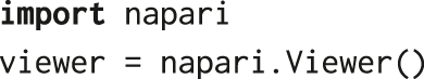
Each stack is stored in the TYX order, where T corresponds to the time axis, and YX are spatial coordinates of the image. To view and interactively browse the stack, we turn to the napari image viewer, which can be accessed programmatically from the notebook. The following code opens a separate viewer window:

The method viewer.add_image() can be then used to add individual stacks as layers in napari, together with the colour map specification and contrast limits:

2.2 Image segmentation

For identifying nuclei from the H2B channel, we use a Python implementation of star-convex object detection for 2D and 3D images, as described in [20]–[22]. The method is based on a convolutional neural network that, for every pixel, predicts a polygon for the cell instance at that position. The package provides a pretrained model, 2D_versatile_fluo, for 2D images of nuclear fluorescent markers. As a preparation step, we create an instance of a pretrained model:

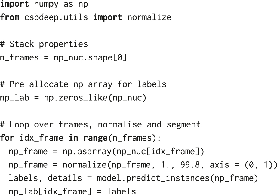
We then pre-allocate a NumPy array of the same size as the image stack, which we will use to store segmentation labels. The input images need to be normalised to the same range as the data used to train the StarDist model, i.e., [0,1]. Therefore, we normalise fluorescence intensities in every frame using normalize from the csbdeep.utils package. Finally, we loop over frames of the H2B channel stack and predict the location of nuclei using StarDist’s model.predict_instances. If no parameters are provided, the prediction step uses a default threshold for the probability, 0.479071, which can be overridden with the prob_thresh parameter.

2.3 Label manipulation

The NumPy array np_lab resulting from the segmentation is a so-called labelled mask. It contains, for every frame, integers denoting object identifiers of nuclei at every pixel location where the StarDist model predicted the nuclei. It will later allow us to extract measurements of individual cells, e.g., fluorescence intensity or area, from the images. However, before proceeding, we process the labels using several functions from the scikit-image library for image processing [23].

First, we remove small labels that correspond to debris or wrong segmentation using the remove_small_objects function from the skimage.morphology utility module of scikit-image. To obtain the final nuclear mask, we set the threshold for the minimum area of nuclei (Figure 3A). The filter threshold min_size = 200 removes all objects comprising less than 200 pixels, which corresponds to a round object of diameter ≈ 16 pixels (5.2 μm).

Figure 3:

Image segmentation. The result of nuclei segmentation with StarDist (A) and identification of cytosolic rings (B) overlaid on nuclear and ERK channels, respectively. (C) Nuclear and cytosolic ring masks.

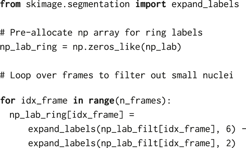
To quantify ERK activity from the ERK-KTR translocation biosensor, we calculate the ratio between the mean cytosolic and nuclear fluorescence intensities, which requires creating an image mask for the cytosol. For every time frame, we perform a series of operations on the existing nuclear mask that create a 4-pixel-wide ring around the nucleus. In the absence of a cytosolic or membrane marker, the ring acts as a proxy for the cytosol. First, we expand the nuclear labels by 6 pixels using expand_labels from skimage.segmentation. Then, we subtract a smaller mask, also obtained from the nuclear mask but only by expanding it by 2 pixels. Rings are 4 pixels wide, with a gap of 2 pixels between the nuclei and rings (Figure 3B).

The exact pixel value by which to expand the nucleus and the thickness of the cytosolic ring depends on cell size and density. Importantly, the ring should minimally overlap with neighbouring cells. We recommend verifying the results visually by plotting the masks on raw images, as in Figure 3A and B.

2.4 Extracting measurements

Having identified labelled masks for nuclei and cytoplasmic rings (Figure 3C), we can now extract properties from the ERK-KTR channel for every labelled region in the field of view. Again, we loop over frames of np_lab_filt and np_lab_ring arrays, and apply regionprops_table from skimage.measure to extract the mean fluorescence intensity, centroid coordinates, and label identifier that allows us to track the nuclei:

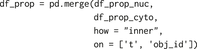
Similar steps, but only with properties = [‘intensity_mean’, ‘label’], yield another pandas data frame, df_prop_cyto, with properties for the cytosolic ring. To obtain a single data frame containing, in a single row, nuclear and cytosolic properties of a cell at a time point, we merge the two tables based on two common key columns: object label ‘obj_id’ and frame number ‘t’ (both integers). To facilitate the merge, we rename the columns in df_prop_nuc and df_prop_cyto generated by regionprops_table, i.e.:

1. l a b e l → o b j _ i d ,

2. i n t e n s i t y _ m e a n → i n t e n s i t y _ m e a n _ n u c and i n t e n s i t y _ m e a n _ c y t o for df_prop_nuc and df_prop_cyto, respectively,

3. c e n t r o i d − 0 → y and c e n t r o i d − 1 → x , which are only present in df_prop_nuc.

Using the pd.merge function, we obtain a single data frame, df_prop, with object label identifiers, positions of nuclear centroids, and nuclear and cytoplasmic fluorescence intensities, from which we can later calculate the cytoplasmic/nuclear ratio, C/N ERK-KTR (Figure 4).

Figure 4:

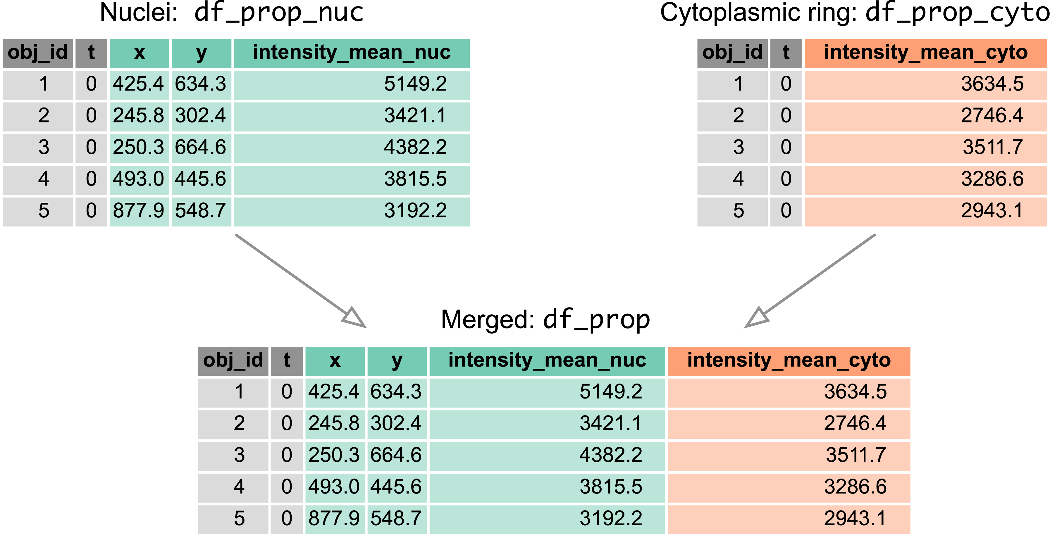
Merging tables. Two pandas data frames containing properties calculated from nuclear and cytoplasmic ring masks, respectively, are merged by two common key columns: object label ‘obj_id’ and frame number ‘t’ (both integers). The resulting ‘df_prop’ contains object label identifiers, positions of nuclear centroids, and nuclear and cytoplasmic fluorescence intensities.

2.5 Tracking

To track single cells over time, we turn to another Python library, btrack [25]. It is a commonly used algorithm that uses objects’ positions and properties, e.g., labels’ area, to reconstruct trajectories in crowded environments such as the confluent epithelium discussed here. For the full code required to track the nuclei, we refer the reader to the Jupyter notebook (Supplementary File 2). Configuration parameters and the motion model for particle tracking are stored in a JSON file (Supplementary File 4), and can be loaded using the configure method of the BayesianTracker class. The parameter of interest to us is the update_method, which we set to BayesianUpdates.APPROXIMATE, which calls a faster, approximate algorithm suitable for larger datasets. The associated parameter, max_search_radius, determines the local spatial search radius. We set it to 70 pixels (22.75 μm), which corresponds to the upper limit of a cell diameter and is sufficient to track frame-to-frame cell displacements encountered in our time-lapse (Figure 3A and Supplementary Video 1). A smaller search radius may fail to track moving nuclei, which results in disjointed segments that should otherwise comprise a single track. When max_search_radius is too large, a single track label may be assigned to different objects in subsequent time frames, thus making measurements extracted from such tracks worthless.

The input data for btrack is a NumPy array with labelled nuclei, np_lab_filt, from which x & y coordinates and the nuclear area are extracted to facilitate tracking. After tracking, btrack outputs a Python list, where each element is a data frame (object of class Tracklet). One such data frame contains a table in long format of a single track, where rows refer to objects in the track at consecutive time points. All those data frames from the list are then merged with the data frame df_prop that contains nuclear and cytoplasmic measurements, using common columns ‘t’ and ‘obj_id’. We thus obtain a data frame df_tracks suitable for the last step of collective event identification with ARCOS. It contains nuclear positions and cytoplasmic/nuclear ERK-KTR ratio measurements in all time frames, with an additional column track_id that holds integer identifiers of tracks/time series. Additionally, btrack provides convenience functions to obtain the data in a format suitable for loading into napari (Supplementary File 2).

Tracking and merging with the measurement table yield single-cell ERK activity time series (ERKATS) (Figure 5A). Several short tracks are still present in the dataset, which may stem from errors in cell segmentation or simply from cells dying during the acquisition (Figure 5B). To perform detrending and binarisation of ERKATS in the next section, we remove time series shorter than 5 h (Figure 5C). This step is required for detrending that applies a long-term median filter with a 2 h window. For a window of that size, time series of at least twice the window length are recommended.

Figure 5:

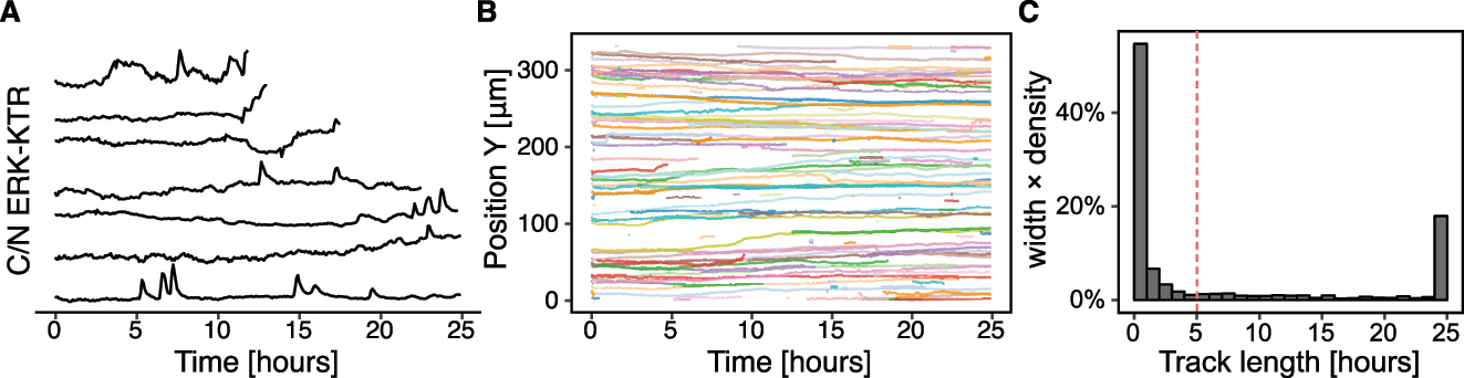
Cell tracking. (A) The result of cell tracking over time with btrack. Each line corresponds to a single cell and its spatio-temporal position. (B) Sample 200 single-cell trajectories projected along the X axis. Note several short tracks. (C) Histogram of track lengths. A vertical dashed line at a 5 h mark indicates a cut-off, below which short trajectories are discarded.

2.6 Collective events

Before we identify collective ERK signalling events with ARCOS, we need to further process ERKATS to remove long-term trends in ERK activity and to identify ERK activity periods, which is the required input for our algorithm. Detrending works in two steps: (1) apply a short-range median filter with a 3-time-point window to remove high-frequency oscillations and incidental peaks due to experimental noise, (2) subtract long-term median-smoothed ERKATS from the time series from step 1. Detrending aims to remove long-term trends due to photobleaching of fluorescent probes, or to remove permanently active cells. The subsequent thresholding of the detrended signal may lead to the identification of longer pulses only during their peak activity, thus omitting the leading and the decaying phase of the pulse (Figure 6A). Both detrending and binarisation, can be performed using a convenience method bin_measurements from the arcos4py package that operates on the ARCOS object defined as:

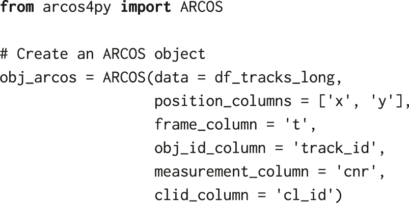
where df_tracks_long is a pandas data frame with single-cell time series obtained from tracking and filtering by length, and the remaining parameters define names of relevant columns, i.e., x & y positions, frame number, track identifier, measurement of the cytoplasmic/nuclear ratio, and cluster identifier that will be determined in the next steps.

Figure 6:

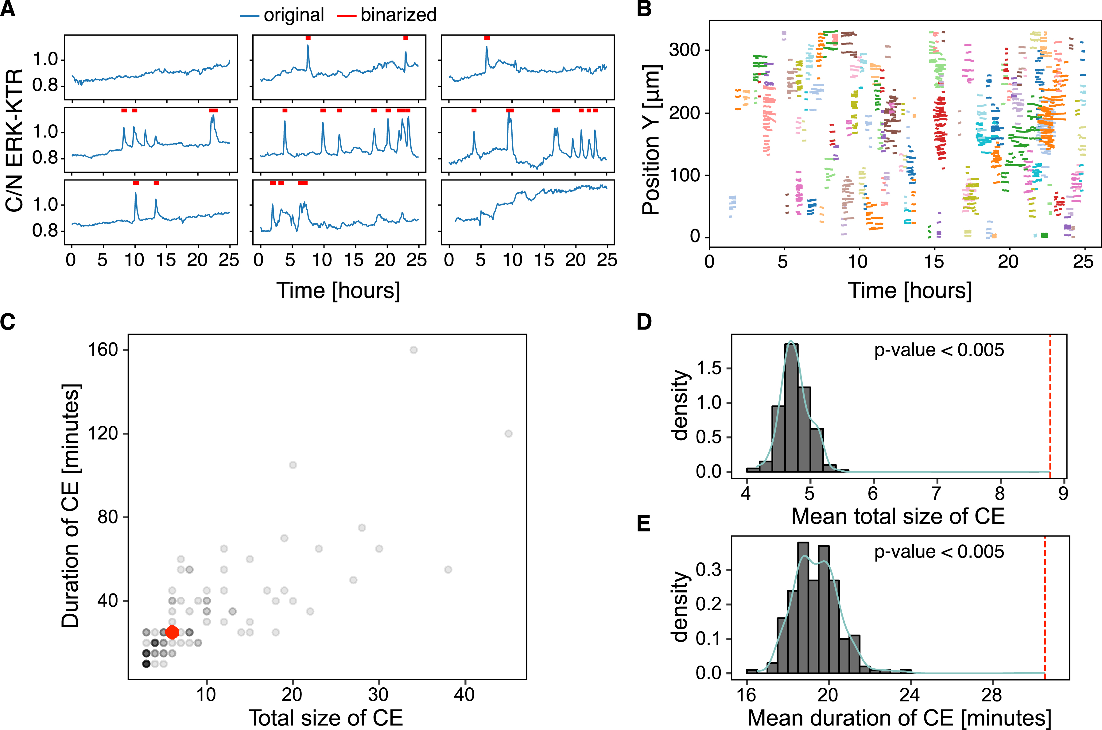
Collective events. (A) Sample detrended and binarised single-cell ERKATS calculated from the cytoplasmic/nuclear ERK-KTR ratio, C/N ERK-KTR. The binarised activity data indicated by red segments is the input for ARCOS. The plot obtained with plotOriginalDetrended from the arcos4py package. (B) Noodle plot visualises CEs identified by ARCOS by projecting them on space-time axes. Each cluster of identically coloured lines corresponds to a single CE, with each line indicating when a single cell participates in the CE. The plot obtained with NoodlePlot from the arcos4py package. (C) Duration versus the mean total number of unique cells in a CE, i.e., “the total size” of a CE. The red dot indicates the median statistics. (D–E) Distributions of statistics calculated from 200 randomisation iterations compared to the observed statistics indicated by the vertical dashed line: the mean total size of CEs (D), and the mean duration of CEs (E). The p-value was calculated as the fraction of cases when the statistic was at least as extreme as observed.

With the following code, and smoothing and thresholding parameters, detrended and binarised ERKATS are added as two additional columns to the input data frame with suffixes resc and bin, respectively:

where smoothK and biasK are window lengths in time points of the short- and long-term median filters, respectively; peakThr is a threshold for detecting peaks in a signal rescaled to [0,1]; binThr is a threshold for final signal binarisation; biasMet is a name of the detrending method. We recommend testing several smoothing/thresholding parameters and verifying the results graphically to obtain the best outcome.

At last, collective events (CEs) are detected and tracked from ERKATS with the code below:

where eps is the search radius in pixels for spatial clustering in individual frames with DBSCAN; minClsz is the minimum number of cells that comprise spatial clusters identified by DBSCAN; nPrev is the number of previous time frames which are used to link spatial clusters in the current time point. The choice of the search radius depends on cell density and the size of clusters of active cells. If set too large, nearby independent CEs are included in a single cluster; too small, and a single CE is identified as several smaller events. A utility function estimate_eps from the arcos4py.tools module helps to estimate eps based on nearest neighbour distances:

The function returns the plot of sorted nearest neighbour distances and the mean, which for our dataset amounts to 44 pixels (14.3 μm). Considering the variability in cell-cell distances, we assume the search radius eps to be 100 pixels, or 32.5 μm, which is approximately twice the mean nearest neighbour distance. When testing smaller values of eps and after inspecting them against raw ERK activity images in the napari image viewer, we obtained fragmented CEs that should belong to a single event. Conversely, larger eps yielded CEs that were assigned a single identifier but stemmed from several independent events.

The noodle plot is a convenient visualisation of collective events projected onto a 2D space-time plane (Figure 6B). Each trace corresponds to a single cell involved in a CE identified by the algorithm, and CEs are coloured by their identifier. The Supplementary Video 1 visualises identified CEs in the raw time-lapse.

2.7 Validation

Statistics such as the mean duration of CEs or the mean total number of unique cells involved in CEs, i.e., “the mean total size”, can be computed from the output of ARCOS (Figure 6C). These observed statistics of CEs can be further tested against a null hypothesis that they do not differ from the statistics of CEs calculated in a system with an equivalent total ERK activity, but with the activation occurring randomly in space and time. The ARCOS package implements 5 randomisation methods to simulate the null hypothesis with varying assumptions. Here, we randomise the time series by shuffling them in space between initial spatial positions of existing time series (cf. Figure S1B in [8]). This method randomises only the spatial component while conserving individual cells’ measurement dynamics and the population-averaged activity over time. By computing the same statistics from the randomised data, we can then calculate the p-value, which is the fraction of cases when the statistic was at least as extreme as the observed statistic.

After importing validation module from the arcos4py package, we randomise the time series:

and calculate the statistics from independent randomisation iterations:

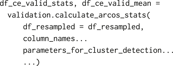
Both functions have the option to execute the calculation in parallel by setting the parameter parallel_processing to True. After repeating the randomisation 200 times, on average, the CEs involved fewer cells and were shorter-lived than the observed average statistics (Figure 6D and E). Since none of the test statistics were at least as extreme as the observed statistic, the p-values for the duration and total size were:

where T is the test statistic, t is the observed value of the test statistic, N _r is the number of independent randomisations from which we obtain the values t _r of the test statistic T [29]–[31].

2.8 Exporting data

Data can be exported at every stage of the analysis. For example, NumPy arrays with labelled masks can be saved as compressed binary files:

and pandas data frames can be exported to compressed CSV files:

The current napari view with blended visible layers can be saved as an RGB TIFF stack using the napari-timestamper package [32]:

3.1 Pre-processing

We begin the analysis by loading the images into napari. If they are in a standard format, such as TIFF files, no additional plugin must be installed. For other file formats, e.g., NIKON nd2, or Leica lif, specific plugins, such as napari-aicsimageio, can be employed.

In the example presented here, TIFF stacks for nuclear and ERK channels, are loaded into napari, and the contrast is adjusted to visualise the individual images properly. The goal is to generate the same two segmentation masks as before, i.e. the ring mask and the nuclear mask, used to measure the fluorescence intensity of the ERK-KTR in the ring and nucleus respectively. As in the Jupyter notebook pipeline, we use StarDist to segment the nuclear channel. Open the stardist-napari plugin and confirm that:

1. The correct image is selected,

2. The “Model Type” is set to 2D,

3. The “Versatile” (fluorescent nuclei) model is selected,

4. The axis order is set to TYX.

Click on “run” to segment the nuclear channel. Once the plugin has finished processing the image stack, it returns the nuclear segmentation as a labels layer and adds it to the viewer.

To create a cytosolic ring, we use the napari-assistant. Said plugin provides a simple interface to set up image processing workflows. The plugins napari-segment-blobs-and-things-with-membranes and napari-pyclesperanto-assistant, provide functions that can be accessed from within the napari-assistant. To use the assistant ecosystem, images must adhere to a standard order of time and space dimensions for inter-plugin communication to work properly. Specifically, image stacks must have the shape TZYX, where T is the time and ZYX are spatial dimensions. Our data comprises 300 time points (frames), 1,024 × 1,024 pixels each. The correct dimension order for the napari-assistant is thus “300,1,1024,1024”. So far, all layers in the napari viewer were loaded as TYX, which outwardly appears to be the same as a 3D stack with the shape ZYX. For the plugin to treat our stack as a time-lapse, an additional, dummy dimension Z needs to be inserted. The napari-assistant also installs a utility plugin napari-time-slicer to perform this conversion. We open a widget called Convert 3D stack to 2D time-lapse from the “Tools > Utilities” section and process every layer with it. Thereafter, all the source layers can be discarded.

We can now set up a workflow that will generate the ring mask. We use the following functions in the order as shown below:

1. Process Labels > Expand Labels; 4 pixel,

2. Process Labels > Reduce Labels to Label Edges,

3. Process Labels > Expand Labels; 2 pixel.

The search bar at the top of the plugin window can be used to quickly find the corresponding functions in the napari-assistant. As input for the first function, select the nuclear segmentation; for the second, select the output from the first function, and so on until a ring is generated.

Using the napari-skimage-regionprops plugin, we measure the mean intensity for the nuclear mask and the ring mask in the ERK-KTR channel. In the “Tools” sub-menu, select “Measurement tables > Regionprops of all frames”. Choose “Intensity” and “Position”. Run this twice, once for the ring, and once for the nuclear segmentation mask. The output from this plugin gets attached to the respective labels layer.

The btrack plugin can be used on the nuclear mask to track our cells. Tracked cells are not required for the analysis with ARCOS; However, they enable more advanced detrending and data analysis down the line. Simply open the plugin and click on “Track”. This will add a “tracks” layer to napari, where we can visually confirm the tracking accuracy.

3.2 Detect collective events

Once we have the measurements for nuclear and cytosolic intensity of the ERK-KTR, we can now load the data into ARCOS and proceed from there. Open the napari ARCOS plugin, then in the first tab, choose the “Load Data From Layers” option. In the selection box, choose both labels-layers that were used to measure cytosolic and nuclear intensity, and if nuclei were tracked using btrack, select the tracks layer in the menu below. Click on “Load Data” and set the names of the columns in the newly opened dialogue. The individual measurements are named after the layers they originate from and what they contain. To calculate the cytosolic to nuclear ratio, in the “Math on first and second Measurement” row choose “Division”, then set the corresponding values in the dialogue box as first and second measurement. Confirm the choices by clicking on “OK” and then select the “ARCOS parameters” tab. Here, set appropriate parameters for your dataset. The epsilon value can be estimated based on the input data. However, in our example, we set it manually. Use the same parameters as outlined in the programmatic approach before. Since we previously converted our TYX image stack to a TZYX stack by adding a Z dimension with size 1, we need ARCOS to also output this dimension order. To achieve this, set the “Output Axis Order” field just below the last ARCOS parameters to “tzyx”, then click on “run ARCOS”. A series of layers will be added to the viewer, containing the detected collective events, their convex hulls, as well as which cells were deemed to be active.

The napari ARCOS plugin provides several interactive plots and tools that help with inspecting and analysing data. Additionally, the parameters used for the analysis, as well as the output and statistics, can be exported, to be used for further analysis and visualisation. The current napari view with blended layers can be exported to an RGB TIFF stack or an MP4 video using a convenient plugin, napari-timestamper [32].

References

[1] P. A. Gagliardi, et al.., “Collective ERK/Akt activity waves orchestrate epithelial homeostasis by driving apoptosis-induced survival,” Dev. Cell, vol. 56, no. 12, pp. 1712–1726.e6, 2021. https://doi.org/10.1016/j.devcel.2021.05.007.Suche in Google Scholar PubMed
[2] T. J. Aikin, A. F. Peterson, M. J. Pokrass, H. R. Clark, and S. Regot, “MAPK activity dynamics regulate non-cell autonomous effects of oncogene expression,” eLife, vol. 9, 2020, Art. no. e60541. https://doi.org/10.7554/eLife.60541.Suche in Google Scholar PubMed PubMed Central
[3] Y. Takeuchi, et al.., “Calcium wave promotes cell extrusion,” Curr. Biol., vol. 30, no. 4, pp. 670–681.e6, 2020. https://doi.org/10.1016/j.cub.2019.11.089.Suche in Google Scholar PubMed
[4] P. Ender, et al.., “Spatiotemporal control of ERK pulse frequency coordinates fate decisions during mammary acinar morphogenesis,” Dev. Cell, vol. 57, no. 18, pp. 2153–2167.e6, 2022. https://doi.org/10.1016/j.devcel.2022.08.008.Suche in Google Scholar PubMed
[5] A. De Simone, et al.., “Control of osteoblast regeneration by a train of Erk activity waves,” Nature, vol. 590, no. 7844, pp. 129–133, 2021. https://doi.org/10.1038/s41586-020-03085-8.Suche in Google Scholar PubMed PubMed Central
[6] K. Aoki, Y. Kondo, H. Naoki, T. Hiratsuka, R. E. Itoh, and M. Matsuda, “Propagating wave of ERK activation orients collective cell migration,” Dev. Cell, vol. 43, no. 3, pp. 305–317.e5, 2017. https://doi.org/10.1016/j.devcel.2017.10.016.Suche in Google Scholar PubMed
[7] N. Hino, et al.., “ERK-mediated mechanochemical waves direct collective cell polarization,” Dev. Cell, vol. 53, no. 6, pp. 646–660.e8, 2020. https://doi.org/10.1016/j.devcel.2020.05.011.Suche in Google Scholar PubMed
[8] P. A. Gagliardi, et al.., “Automatic detection of spatio-temporal signaling patterns in cell collectives,” J. Cell Biol., vol. 222, no. 10, 2023, Art. no. e202207048. https://doi.org/10.1083/jcb.202207048.Suche in Google Scholar PubMed PubMed Central
[9] S. Regot, J. J. Hughey, B. T. Bajar, S. Carrasco, and M. W. Covert, “High-sensitivity measurements of multiple kinase activities in live single cells,” Cell, vol. 157, no. 7, pp. 1724–1734, 2014. https://doi.org/10.1016/j.cell.2014.04.039.Suche in Google Scholar PubMed PubMed Central
[10] M. Dobrzyński, “Source data and python scripts,” 2024. Available at: https://data.mendeley.com/datasets/z29fyn6kzz.Suche in Google Scholar
[11] T. Kluyver, et al.., “Jupyter notebooks – a publishing format for reproducible computational workflows,” in Positioning and Power in Academic Publishing: Players, Agents and Agendas, F. Loizides, and B. Schmidt, Eds., IOS Press, 2016, pp. 87–90.Suche in Google Scholar
[12] G. Van Rossum and F. L. DrakeJr., Python Reference Manual, Amsterdam, Centrum voor Wiskunde en Informatica, 1995.Suche in Google Scholar
[13] M. Dobrzyński, “Source python scripts,” 2024. Available at: https://github.com/dmattek/ARCOS-tutorial.Suche in Google Scholar
[14] N. Sofroniew, et al.., “napari/napari: 0.4.15rc1,” 2022. Available at: https://zenodo.org/record/3555620.Suche in Google Scholar
[15] B. Grädel, “arcos4py: automated recognition of collective signalling for python,” 2024, Available at: https://github.com/bgraedel/arcos4py.Suche in Google Scholar
[16] C. R. Harris, et al.., “Array programming with NumPy,” Nature, vol. 585, no. 7825, pp. 357–362, 2020. https://doi.org/10.1038/s41586-020-2649-2.Suche in Google Scholar PubMed PubMed Central
[17] W. McKinney, “Data structures for statistical computing in Python,” in Proceedings of the 9th Python in Science Conference, S. van der Walt, and J. Millman, Eds., 2010, pp. 56–61.10.25080/Majora-92bf1922-00aSuche in Google Scholar
[18] C. Gohlke, “tifffile,” 2024. Available at: https://doi.org/10.5281/zenodo.10651760.Suche in Google Scholar
[19] Joblib Development Team, “Joblib: running python functions as pipeline jobs,” 2020. Available at: https://joblib.readthedocs.io/.Suche in Google Scholar
[20] U. Schmidt, M. Weigert, C. Broaddus, and G. Myers, “Cell detection with star-convex polygons,” in Medical Image Computing and Computer Assisted Intervention – MICCAI 2018 – 21st International Conference, Granada, Spain, September 16-20, 2018, Proceedings, Part II, 2018, pp. 265–273.10.1007/978-3-030-00934-2_30Suche in Google Scholar
[21] M. Weigert and U. Schmidt, “Nuclei instance segmentation and classification in histopathology images with stardist,” in The IEEE International Symposium on Biomedical Imaging Challenges (ISBIC), 2022.10.1109/ISBIC56247.2022.9854534Suche in Google Scholar
[22] M. Weigert, U. Schmidt, R. Haase, K. Sugawara, and G. Myers, “Star-convex polyhedra for 3d object detection and segmentation in microscopy,” in The IEEE Winter Conference on Applications of Computer Vision (WACV), 2020.10.1109/WACV45572.2020.9093435Suche in Google Scholar
[23] S. Van der Walt, et al.., “scikit-image: image processing in python,” PeerJ, vol. 2, p. e453, 2014. https://doi.org/10.7717/peerj.453.Suche in Google Scholar PubMed PubMed Central
[24] Open-source community, “py-clesperanto: a multi-language framework for GPU-accelerated image processing,” 2024. Available at: https://pypi.org/project/pyclesperanto/.Suche in Google Scholar
[25] K. Ulicna, G. Vallardi, G. Charras, and A. R. Lowe, “Automated deep lineage tree analysis using a bayesian single cell tracking approach,” Front. Comput. Sci., vol. 3, p. 92, 2021. https://doi.org/10.3389/fcomp.2021.734559.Suche in Google Scholar
[26] J. D. Hunter, “Matplotlib: a 2d graphics environment,” Comput. Sci. Eng., vol. 9, no. 3, pp. 90–95, 2007. https://doi.org/10.1109/MCSE.2007.55.Suche in Google Scholar
[27] QuantStack, “Mamba: a fast, robust, and cross-platform package manager,” 2020, Available at: https://mamba.readthedocs.io.Suche in Google Scholar
[28] L. P. Coelho, “Mahotas: open source software for scriptable computer vision,” J. Open Res. Softw., vol. 1, no. 1, p. e3, 2013. https://doi.org/10.5334/jors.ac.Suche in Google Scholar
[29] A. C. Davison and D. V. Hinkley, Bootstrap Methods and their Application, Cambridge University Press, 2013.Suche in Google Scholar
[30] P. Good, Permutation, Parametric and Bootstrap Tests of Hypotheses, New York, Springer Series in Statistics. Springer-Verlag, 2004.Suche in Google Scholar
[31] B. F. J. Manly and J. A. Navarro Alberto, Randomization, Bootstrap, and Monte Carlo Methods in Biology. Texts in Statistical Science, 4th ed. Boca Raton, FL, Chapman & Hall/CRC, 2022.Suche in Google Scholar
[32] B. Grädel, “Napari time stamper plugin,” 2024. Available at: https://github.com/bgraedel/napari-timestamper.Suche in Google Scholar
[33] B. Grädel, “ARCOS napari GUI,” 2024. Available at: https://www.napari-hub.org/plugins/arcos-gui.Suche in Google Scholar
[34] R. Haase, “devbio-napari: a bundle of napari plugins useful for 3D+t image processing and analysis for studying developmental biology,” 2024. Available at: https://www.napari-hub.org/plugins/devbio-napari.Suche in Google Scholar
[35] N. L. DeCuzzi, et al.., “Spatiotemporal clusters of ERK activity coordinate cytokine-induced inflammatory responses in human airway epithelial cells,” bioRxiv preprint, 2024, https://doi.org/10.1101/2024.02.03.578773.Suche in Google Scholar PubMed PubMed Central
[36] K. W. Pond, et al.., “Live-cell imaging in human colonic monolayers reveals ERK waves limit the stem cell compartment to maintain epithelial homeostasis,” eLife, vol. 11, 2022, Art. no. e78837. https://doi.org/10.7554/eLife.78837.Suche in Google Scholar PubMed PubMed Central
[37] E. C. Greenwald, S. Mehta, and J. Zhang, “Genetically encoded fluorescent biosensors illuminate the spatiotemporal regulation of signaling networks,” Chem. Rev., vol. 118, no. 24, pp. 11707–11794, 2018. https://doi.org/10.1021/acs.chemrev.8b00333.Suche in Google Scholar PubMed PubMed Central
[38] E. Strickland, et al.., “Self-extinguishing relay waves enable homeostatic control of human neutrophil swarming,” bioRxiv preprint, 2023. https://doi.org/10.1101/2023.06.27.546744.Suche in Google Scholar PubMed PubMed Central
[39] S. B. David, K. Y. Ho, G. Tanentzapf, and A. Zaritsky, “Formation of recurring transient ca2+-based intercellular communities during drosophila hematopoiesis,” bioRxiv preprint, 2023. https://doi.org/10.1101/2023.11.25.568594.Suche in Google Scholar
Supplementary Material
This article contains supplementary material (https://doi.org/10.1515/mim-2024-0003).
© 2024 the author(s), published by De Gruyter on behalf of Thoss Media
This work is licensed under the Creative Commons Attribution 4.0 International License.
Artikel in diesem Heft
- Frontmatter
- Editorials
- Empowering the Microscopy Community: Welcome to the Inaugural Issue of Methods in Microscopy
- Embracing innovation in microscopy
- News
- Microscopy Community News
- Special Issue: Volume Microscopy Across Scales
- View
- Array tomography: trails to discovery