Design of Optimized Multiobjective Function for Bipedal Locomotion Based on Energy and Stability
-
Manish Raj
 und
Gora C. Nandi
und
Gora C. Nandi

Abstract
This paper presents a novel analytical method to develop the multiobjective function including energy and stability functions. The energy function has been developed by unique approach of orbital energy concept and the stability function obtained by modifying the pre-existing zero moment point (ZMP) trajectory. These functions are optimized using real coded genetic algorithm to produce an optimum set of walk parameters. The analytical results show that, when the energy function is optimized, the stability of the robot decreases. Similarly, if the stability function is optimized, the energy consumed by the robot increases. Thus, there is a clear trade-off between the stability and energy functions. Thus, we propose the multiobjective evolutionary algorithm to yield the optimum value of the walk parameters. The results are verified by Nao robot. This approach increases the energy efficiency of Nao robot by 67.05%, and stability increases by 75%. Furthermore, this method can be utilized on all ZMP classed bipeds.
1 Introduction
Bipedal locomotion is still an open-ended problem and poses great challenges to researchers from various backgrounds. One of the reasons responsible for the sluggish development of bipedal machines, is the need for simultaneously achieving two objectives, i.e. higher energy efficiency and greater stability, both of which are important attributes of an autonomous robot. The flat footed bipedal robots ensures greater stability but at an expense of consuming more energy [19]. On the other hand, the point footed bipedal robots consume significantly less amount of energy as compared to flat footed robots, sacrificing the stability concerns required for performing tasks other than walking. Most of the humanoid robots today are flat footed, because of the versatility of tasks being performed by them other than walking. The flat footed robots use the concept of zero moment point (ZMP) [18] to ascertain stability during different phases of walking. From the above discussions, it can be inferred that there is a clear trade-off between the energy consumed by the robot and its stability issues. That is, the higher the energy consumed by the robot, the more stable it is and vice versa. Therefore, current research trends towards building efficient algorithms that balance the trade-off between the two contrasting objectives.
In the past, there has been significant contributions in developing energy efficient bipedal robots and optimizing their gait parameters using evolutionary algorithms. It was seen that the demerit of the robots employing ZMP is that they consume a lot of energy. The basic reason behind the enormous consumption of energy is the large gap between the artificial gait synthesized in bipeds and the natural human gait. The amount of energy consumed during walking depends on the type of gait pattern of a person [13].[1] The gait pattern plays a vital role in bipedal walking. This is because it determines the optimal footholds, velocity and acceleration of the support foot. This, in turn, affects the robot’s dynamic stability, energy consumption, harmony and so on. In short, the quality of the legged locomotion is decided by its gait pattern [8]. Thus, carefully designing the gait pattern of the bipeds may help a lot in reducing the energy consumption as well as increasing its stability [19]. This section discusses the research carried out in the field of gait optimization in order to decrease the energy consumed by the robot as well as increase its stability.
Despite the huge time taken by the evolutionary algorithms for optimization, the gait optimization is generally performed by using genetic algorithm (GA), due to its robustness in search and optimization problems [7]. This is because most of the ZMP classed bipedal robots have offline walking pattern generation. So in order to design an energy efficient gait, the optimization is carried out before the actual walking starts. Some of the contributions related to gait optimization is worth mentioning here. Capi et al. [2] used real coded genetic algorithm (RCGA) to optimize the energy consumed by the robot. The objective was to find the joint trajectories, which consume minimum energy. The energy function was formulated by integrating the torque generated at the motor joints. It was a single objective optimization problem, where only energy was optimized. The stability criterion was used for imposing constraint on the energy function. That is, if the position of ZMP goes outside the support polygon, the energy function was heavily penalized. The drawback of this research was that it did not explicitly specify the ZMP trajectory, which accounts for the biped’s stability. Capi et al. [3] synthesized the gait pattern of a biped, using GA and radial basis function neural network (RBFNN). The approach used GA first to find the optimal set of gait parameters, which was then used to train the RBFNN, in order to generate real time energy efficient gait pattern. However, due to the large computational overhead, this method suffered significant delays in real time applications. Park and Choi [16] used GA to minimize energy consumed by a 6-DoF bipedal robot, by selecting optimal locations of the mass centers of the links. However, this method requires one to design a bipedal robotics hardware, in such a manner that the locations of Center of Mass (CoM) of each link corresponds to optimal locations of CoM previously found, using GA. Choi et al. [4] used GA to optimize the walking trajectory of IWR-III bipedal robot by minimizing the sum of deviations of velocities, accelerations and jerks in order to maintain continuity of joint trajectories and energy distribution at the via points. But this research does not show how implementing continuity in the joint trajectory results in the improvement of energy consumption. An analysis of [12] reveals that variation of the walk parameters as well as the stiffness values of the joints affects the energy consumed by Nao. Experiments were performed on reducing the knee flexion and stiffness values of the joints. However, a formal mathematical proof of the reduced energy consumption is missing. Moreover, the energy efficiency is reported to have increased by 59%. In [17], Sun and Roos employ policy gradient reinforcement learning (PGRL) and improve the power efficiency of Nao by 44%. A critique of [17] reveals that it does not take into account the different states of walking like transition from double support phase (DSP) to single support phase (SSP), effect of impacts etc., which is critical when studying energy consumption. Also, the height of CoM is not taken into account in [17], which is important for analyzing the dynamics of the Linear Inverted Pendulum Model based humanoid robot like Nao, ASIMO etc.
Besides energy consumption, another major concern in bipedal locomotion is its stability [10]. The ZMP concept had been heavily relied on by researchers for ensuring stability of bipedal robots [11]. Ames et al. [1] used optimization to modify the gait parameters of Nao robot such that the least squares fit of the robotic walking data approximates to the human walking data subjected to the constraints that satisfy partial hybrid zero dynamics. Lin and Peng [14] proposed a dynamic balancing method for bipedal robots using cerebellar model arithmetic computer neural network. The advantage of this method was that it could fetch optimized gait parameters in real time, according to the terrain profile. Miller [15] developed improved control algorithms for a bipedal robot that increased its stability. In particular, Miller modelled the gait as a simple oscillator, applied Proportional Integrated Deferential control algorithm and then performed neural network training.
The novelty of this paper extends to three folds. The concept of orbital energy has been used to develop an energy function which indicates the energy consumed by the robot in one gait cycle. Secondly, this paper proposes a new function which gives a measure of the stability of the bipedal robot not only during the SSP but also during the transition from the SSP to DSP and vice versa. The work mentioned in [15] has attempted to build a stability function, which had only taken the stability concern of the robot during the SSP. And finally, this is probably the first paper that applies multiobjective evolutionary algorithm on Nao humanoid robot. The advantage of such an approach is that the theoretical results can be verified on a real Nao robot.
2 Stability Parameters of Bipedal Robots: ZMP and CoM
In this section, We first introduce the notion of two important concepts used throughout this paper, i.e. ZMP and CoM. The ZMP is defined as a point on the walking surface at which the resultant moment caused by the active forces (gravitational, centrifugal and Coriolis forces) is equal to zero. On the other hand, CoM is defined as a point where the entire mass of the system is assumed to be concentrated. In order to maintain stability during walking, the ZMP should lie within the support polygon. That means when the robot is in the SSP the ZMP lies at the center of the foot. On the other hand, when the robot is in the DSP, the ZMP lies in the center of the convex hull formed by the two supporting feet.
2.1 Ideal ZMP and CoM Trajectories
An ideal walk of Nao robot with a fixed step size B is shown in Figure 1A. The x- and y-components of ZMP trajectories with respect to time is shown in Figure 1, where A is half of the lateral distance between the feet. Mathematically, the horizontal components of the ZMP trajectories can be expressed as

Ideal Nao ROBOT’s Walk and ZMP Trajectories.
(A) Nao’s footprints showing ideal walking. (B) The x-component of ZMP trajectory. (C) The y-component of ZMP trajectory.
where T is the half period time. The x- and y-components of ZMP trajectory, shown in Figure 1B, is quite intuitive. The x-component of ZMP is a staircase because, as the robot switches its support from the left leg to the right leg or vice versa, the CoM effectively increments by a magnitude of the step size (B). Similarly, for the y-component of the ZMP, the upper and the lower edges of the square wave, as shown in Figure 1C, corresponds to the ZMP trajectory in the left and the right legs, respectively. However, the above specified trajectories are not realistic. This is because Eqs. (1) and (2) assume instantaneous exchange of support foot. This assumption can be noticed from the instant change in the ZMP trajectory in Figure 1B and C.
2.2 Realistic/Practical ZMP-CoM Trajectories
Ideally, the ZMP shifts instantly from the support polygon of the left foot to the support polygon of the right foot during the transition from the DSP to SSP. But in a practical case, a slight modification of the ZMP trajectory was suggested by [5]. Instead of the ZMP shifting instantly, the ZMP follows the CoM during the transition from the DSP to SSP as shown in Figure 2. The X-directional ZMP trajectory is given by

Practical ZMP and CoM Trajectories.
(A) The x-directional ZMP and CoM trajectory. (B) The y-directional ZMP and CoM trajectory.
where B is the step length, ts is the transition time required to change from DSP to SSP, and T is the half period time required to complete one step. Mathematically, T represents the time required by the biped to switch from DSP to SSP and then again back to DSP. During the DSP, i.e. (0≤t≤ts ) and (T–ts ≤t≤T), the CoM trajectory follows the ZMP trajectory.
During the SSP, i.e. (ts <t<T–ts ) the CoM trajectory is defined by the equation
where
Using the initial and the final conditions, the values of C1, C2 and, kx are
The Y-directional ZMP trajectory is given by
where A is the distance between the left foot and the right foot. During the DSP, i.e. (0≤t≤ts ) and (T–ts ≤t≤T), the CoM trajectory follows the ZMP trajectory.
During the SSP, i.e. (ts <t<T–ts ) the CoM trajectory is defined by the equation
The solution of Eq. (9) is given by
Using the initial and the final conditions, the values of C3, C4 and, ky are
However, Eqs. (6) and (10) involve hyperbolic terms, which are unbounded and are difficult to be realized. Therefore, an approximate solution is formulated by expressing the ZMP trajectories by Fourier series [6]. Since
The x-component of ZMP trajectory(shown in Figure 1B) is not periodic in nature, and its Fourier series cannot be found. An approximate analysis was given in [6] to calculate the Fourier series of
Once the ZMP and CoM trajectories are formed, we use them to build up the energy and stability equation at different support phases.
3 Formulation of the Objective Function
3.1 The Energy Function
Mostly, the energy functions derived for a bipedal robot uses the concept of the change in torque at the joints [2], [8]. In this work, the authors have developed an energy function using the concept of orbital energy. The derivation of energy function is valid for Nao robot because the Nao robot’s hip trajectory (representing CoM) follows a straight line while walking, maintaining a constant height above the ground (the only major requirement for the application of the orbital energy concept).
A generalized equation can be written as
where
The robot was made to walk for one complete gait cycle. The walking cycle was divided into three different phases: DSP, SSP and DSP.
Case 1: 0≤t≤ts
During this time interval, the robot is in DSP. The CoM and ZMP trajectories are almost similar which is given by Eqs. (4) and (8). The equation for orbital energy can therefore be obtained by substituting the values of xcm and ycm in Eqs. (37) and (38) as
Substituting xcm(1)=xcm and ycm(1)=ycm from the equation and
Case 2:ts ≤t≤T–ts
During this time interval, the robot is in SSP. The CoM and ZMP trajectories are different and is given by
The equation for orbital energy during this time interval can be obtained by substituting the values of xcm and ycm mentioned above in Eqs. (37) and (38).
Substituting xcm(2)=xcm and ycm(2)=ycm from Eqs. (18) and (19) and
Case 3:T–ts ≤t≤T
During this time interval, the robot is again in DSP, thus completing one complete gait cycle. The CoM and ZMP trajectories are almost the same as mentioned in Case 1. However, the values of xcm and ycm change as shown in Figure 2 and is given by
Substituting xcm(3)=xcm and ycm(3)=ycm from Eqs. (22) and (23) and
From the above discussions, it can be concluded that energy is a function of xZMP, yZMP, zcm and ts . The coordinates of CoM and ZMP in turn depends on the value of walk parameters step length B and lateral foot distance B.
The energy function, therefore, is
The aim is to minimize the energy consumed, given by Eq. (26), subjected to the constraints specified by Aldebaran Robotics (manufacturer of Nao robot):
3.1.1 Optimization of the Energy Function – Results
RCGA is used to optimize the energy function given by Eq. (26), subjected to the constraints to the walk parameters mentioned above. This section shows the default as well as the optimized energy plots of the Nao robot. Corresponding to the optimized walk parameters, the energy plot obtained is also compared with the PGRL and stiffness based approach for calculating the energy of the robot. Finally, the joint trajectories of the hip and knee joint of the bipedal robot, ensuring minimum energy consumption, is generated.
The default Aldebaran walk engine [9] had the values of input parameters set as
The energy plot of the default Aldebaran walk over a time period T is shown in Figure 3A. Using Eq. (26), the energy consumed by the robot during walking was 0.0261 J. Figure 3A shows that the energy consumed by the robot initially is high. A discontinuity in the energy graph is seen at time t=ts =0.41 s, when the robot transitions from DSP to SSP. During the SSP, i.e. 0.4<t<0.82, the energy function is sinusoidal in nature. This is because the COM trajectory given by Eqs. (11) and (12) includes sinusoidal terms. For simplicity, we have taken harmonics only upto the second order. If the harmonics are increased, the number of peaks appearing during this interval in the energy graph will also increase subsequently. At t=0.82 (T–ts ), the robot transitions to DSP. During this interval, the energy graph is similar to the DSP, which was encountered at the start of the gait cycle. Figure 3B shows the hip and the knee trajectories of a real Nao robot using default walk parameters.

Energy Plot and Joint Trajectories of Default Walk.
(A) Energy plot using default Aldebaran walk parameters. (B) Default hip and knee trajectories of Nao.
The objective function was then optimized by using GA. The results obtained by using GA is shown in Figure 4. The top left plot shows how the fitness function (objective function) gradually converges to a global minimum value. The best fitness value obtained using GA is 0.00854 J. The optimized value of the four walk parameters are shown in the top right figure. Due to different constraints of walk parameters, the values of walk parameters are normalized, such that they lie between the given constraints. For example, ts =1 shown in Figure 4 means ts is at the upper extrema of the constraint for ts (ts =0.6). By using GA, at the end of 51 iterations, the optimized values of the parameters are

Energy Optimization using GA.
The energy plot of the optimized walk is depicted from the bottom right figure. When the above optimized walk parameters were substituted in Eq. (26), the energy consumed by the robot was 0.0085 J. This marked an increased power efficiency of Nao robot by 69.35%. This is an improvement over results reported in [12] and [17] which propose increased power efficiency by 44% and 59%, respectively.
The simulations were carried out in Choregraphe software as shown in Figure 5A. The optimized walk parameters were tested on a real Nao robot, and the corresponding hip and knee trajectories were generated as shown in Figure 5B. It can be clearly noticed from Figures 3B and 5B that the hip trajectory is close to zcm. Also, the optimized joint trajectory has more peak to peak deviations as compared to the the default joint trajectories. This is because the value of the walk parameter ts of a Nao robot cannot be directly controlled. Instead, ts can be controlled by adjusting the value of step height (h) walk parameter. The default hip trajectory has less deviations since step height is set to minimum (h=0.005 m). On the other hand, the optimized hip trajectory has more deviations since the step height was increased to h=0.04 m, thereby increasing the value of ts . Figure 6A shows the energy plot obtained by setting the optimized value of walk parameters obtained from different algorithms like PGRL, stiffness based walking, RCGA, and default Aldebaran walking. Figure 6B shows that when Nao robot was made to walk for one gait cycle, the energy consumed was 0.0261 J. The stiffness of the motor joints were varied in [12], and the energy consumed is reported to be 0.011 J. On applying optimization techniques like PGRL [17], the energy consumed by Nao robot was reported to be 0.014 J. By applying RCGA to our energy function, the energy consumed by the robot was 0.0085 J. This marks an increase in energy efficiency of the Nao robot by 69.35% over default Aldebaran walk, 15.35% over PGRL based walk, and 10.35% over stiffness based walk.

Simulation of Nao’s Walking in Choregraphe and Optimized Walk Trajectories.
(A) Nao simulation in Choregraphe. (B) Optimized hip and knee trajectories of Nao.
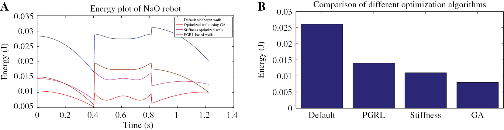
Comparison of Different Optimization Algorithms.
(A) Energy plot of Nao using different optimization algorithms. (B) Comparison of energy consumption over one gait cycle.
3.2 The Stability Function
The ZMP position must be at the center of support polygon of the bipedal robot, in order to ascertain maximum stability. Recent works on formulating a stability function [2] had used the concept of ZMP deviation from the mean position. That is, the stability function indicates the measure of deviation of the calculated ZMP position (calculated from the real robot’s dynamics) from the desired ZMP position (at the center of the support polygon). However, the stability functions proposed earlier requires the ZMP trajectory to be at the center of the robot’s foot only during the SSP. It is a well-known fact that a normal gait cycle consists of alternate phases of DSP and SSP. Therefore, the consideration of DSP in designing the stability function plays an equally important role. In this work, the author has considered both the support phases of walking, i.e. DSP and SSP. The main idea behind the proposal of this novel stability function is that the ZMP trajectory remains in the center of the support polygon not only during the SSP but also during the DSP.
3.2.1 Derivation of the Stability Function
The stability function (ζ) is given by the difference of the y-component[2] of calculated ZMP position ZMPcalc given by Eq. (7) (explained in Section 2.2) and the desired ZMPdes (explained in this section). Mathematically, this can be represented as:
Lower values of ζ indicate that the robot is highly stable, ensuring that the ZMP trajectory remains at the center of the support polygon in both DSP and SSP. Higher values of ζ state that there is a large deviation of the calculated ZMP from the desired ZMP, indicating that the robot is unstable. The green dashed line in Figure 7 shows the desired ZMP trajectory. The red solid line indicates the calculated ZMP trajectory which is the same as the one explained earlier. The blue line represents the CoM trajectory of the bipedal robot. Since ZMPcalc is defined by Eq. (7), the only unknown in Eq. (27) is ZMPdes. Similar to the Energy function derived in Section 3.1, the ZMP trajectory is modified and its equation is formulated in different time intervals.

CoM, Calculated ZMP and desired ZMP Trajectories of a Bipedal Robot.
Case 1: 0≤t≤ts
During this interval, the bipedal robot is in transition from DSP to SSP. The ZMP trajectory (indicated by green dashed line) is parallel to the ZMP trajectory obtained during the interval T+1.5ts ≤t≤2T+ts . Thus,
At t=ts ,
During this interval, the equation for
Case 2:ts ≤t≤1.5ts
During this time interval, the desired ZMP trajectory is the same as the calculated ZMP trajectory. The ZMP position shifts from the heel towards the center of the foot. That is,
During this interval, the equation for
Case 3: 1.5ts ≤t≤T+ts
Instead of the ZMP shifting towards the toe, during this interval, the ZMP trajectory is a straight line which is parallel to the sides of the support polygon formed by the left and the right feet. The slope of the dashed line (green) is given by
Thus, the equation of this line can be written as
From the graph shown in Figure 7, at time
During this interval, the equation for
During the interval, T–ts ≤t≤T, the equation for
Combining Eqs. (28), (30) and (32) into one single piece-wise equation, the equation for
Once the equation for
Once the stability function is formulated, the aim is to minimize the average value of ζ over the gait cycle T subjected to the constraints on the walk parameters specified by Aldebaran Robotics (manufacturer of Nao) as
The minimization of ζ means that the ZMP trajectory remains at the center of the support polygon throughout the walking cycle. In order to realize the ZMP trajectory given by Eq. (35) on a real Nao robot, the CoM equation needs to be computed by inputting the ZMPdes equations into Eq. (11).
3.2.2 Optimization of the Stability Function – Results
The stability function given by Eq. (36) is optimized using RCGA subjected to the constraints on the walk parameters mentioned above. This section illustrates the default as well as the optimized stability plots of the Nao robot.
The default Aldebaran walk engine [9] had the values of the input parameters of Nao robot set as
The stability plot of the default Aldebaran walk over one gait cycle is shown in Figure 8. Using Eq. (36), the average stability of the bipedal robot over one gait cycle was measured to be 0.0124. The numerical value just stated indicates the average degree of deviation of the ZMPdes from the ZMPcalc trajectory. From Figure 8, it can be inferred that when the robot is switching to DSP, the stability of the robot increases. This can be seen from the decreasing value of ζ during the interval 0≤t≤0.41. The robot comes to complete DSP during the interval 0.41≤t≤0.6. During this time interval, the robot possesses maximum stability (ζ=0). In the next time interval 0.6≤t≤0.82, the robot switches to SSP. The SSP is a highly unstable state. This can be seen from the sudden rising value of ζ as shown in Figure 8. During the time interval 0.82≤t≤1.25, the robot is again switching to DSP. The stability of the robot increases during this time interval. This is indicated by the decreasing value of ζ, as shown in Figure 8.
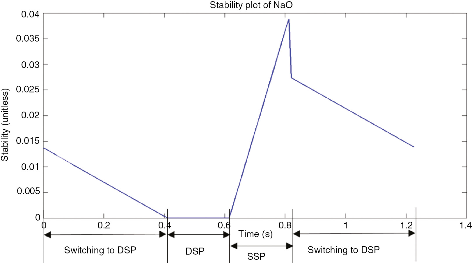
Stability Plot using Default Aldebaran Walk Parameters.
The stability function was then optimized using RCGA. The results obtained by using GA is shown in Figure 9. The top left plot shows how the fitness function (minimizing the stability function) gradually converges to a global minimum value. The best fitness value obtained using GA is 0.0028. The optimized value of the walk parameters is shown by means of a bar graph in the top right plot. It is seen that by the end of 51 iterations, the optimized value of the walk parameters are

Optimization of Stability Function using RCGA.
The stability plot of the optimized walk is depicted from the bottom right figure. Substituting the above walk parameters in Eq. (36), the value of ζ obtained is 0.0028. This marks an increase in the stability of the bipedal robot by 77.42% over the existing ζ value obtained using default walk parameters. The stability plot of Nao, shown in Figure 9 shows that the robot is highly stable during its transition from DSP to SSP. The robot becomes unstable during SSP, which is quite normal. It is observed that with the implications of the optimized walk parameters on the robot, the stability of the biped increases. This is due to the sudden decrease in the value of ζ during the transition of DSP to SSP and vice versa as shown in Figure 9.
4 Multiobjective Optimization Problem
The use of the optimization was greatly felt during World War I, when the demand for the number of products (weapons, processed food etc.) exceeded the production capacity of industries. Due to ongoing war, resulting in time crisis, new factories could not be set up to meet the demands of the public. This gave rise to a method called optimization, first introduced by Fermat and Lagrange, where the existing facilities of the factories were used wisely (by altering the value of input parameters) so as to maximize the yield using the pre-existing state of the art. Optimization may be broadly classified into two categories based on the number of objectives to be optimized. They are (a) single objective optimization and (b) multiobjective optimization.
Single objective optimization: In this method, there is only one objective function which needs to be optimized. For instance, both the functions (energy and stability) derived in Section 3 were optimized separately. That is, when the energy function given by Eq. (26) was optimized using RCGA, it yielded a different set of optimum walk parameters as compared to those obtained from the optimization of the stability function given by Eq. (36).
To illustrate the effect of single objective optimization, consider Table 1, where the optimized walk parameters obtained for energy function is applied to the stability function. Table 1 shows the default as well as the optimized walk parameters obtained from the optimization of the energy function. The optimized walk parameters were substituted in the stability function, and the resulting value of the stability is noted. Figure 10A shows the optimized energy plot of Nao robot. By using the optimized walk parameters (obtained by applying RCGA on the energy function), the stability plot of Nao robot is generated. It can be noted from Table 1 that the optimized walk parameters give a minimum energy consumption of 0.0085 J, but the same parameters yield stability value as 0.0037. The stability function was optimized in Section 3.2, whose optimum value came to be 0.0028. Thus, it can be seen here that only one objective could be satisfied.
To further exemplify the meaning of single objective optimization, consider the reverse case, where the stability optimized walk parameters are applied to the energy function. Table 2 shows that the value of energy consumed by the robot differs from the optimized energy value shown in Figure 1, when stability optimized walk parameters are applied on energy equation given by Eq. (26). Figure 11A shows the energy plot obtained for a bipedal robot using stability optimized walk parameters. It can be clearly seen from Table 2 that the energy function does not yield optimum value (E=0.0085 J), when the stability optimized walk parameters are applied on the energy equation. On the other hand, the stability function has been optimized here, which yields a minimum value of 0.0028.
Thus, from the above discussions, it is clear that the energy and stability of the robot can be best optimized when they are handled singly. This concept of applying optimization separately on different objective functions is known as single objective optimization.
Multiobjective optimization: In this kind of optimization problems, there are more than one objective functions. Consider for instance the problem of stability and energy consumption of the bipedal robot. Since both the functions (energy and stability) have to be applied on the same bipedal robot, the user needs a single set of walk parameters that can optimize both energy consumption and the stability of the robot at the same time. However, it was seen in the previous section that the optimization of one function leads to worsening of the other. In particular, when the energy function of the robot was optimized, the stability of the robot decreased (high value of ζ). Also, the optimization of the stability function ended up in greater energy consumption by the robot. Thus, the two functions are clearly contrasting in nature. The drawback in such cases is that there is no single best solution. To encounter such problems, a set of such optimal solutions are found, each satisfying the desired objectives to a certain degree. The problem of handling this problem is discussed in detail in Section 4.1.
Energy Optimized Walk Parameters Applied on Energy and Stability Functions.
| ts | zcm | A | B | Energy (J) | Stability | |
|---|---|---|---|---|---|---|
| Default | 0.41 | 0.25 | 0.135 | 0.04 | 0.0261 | 0.0124 |
| Optimized | 0.6 | 0.161 | 0.101 | 0.01 | 0.085 | 0.0037 |

Effect of Energy Optimized Walk Parameters on Energy and Stability Functions.
(A) Optimization of the energy function. (B) Stability plot using the energy optimized walk parameters.
Stability Optimized Walk Parameters Applied on Energy and Stability Functions.
| ts | zcm | A | B | Energy (J) | Stability | |
|---|---|---|---|---|---|---|
| Default | 0.41 | 0.25 | 0.135 | 0.04 | 0.0261 | 0.0124 |
| Optimized | 0.5761 | 0.1732 | 0.1059 | 0.0469 | 0.0148 | 0.0028 |

Effect of Stability Optimized Walk Parameters on Energy and Stability Functions.
(A) Energy plot using the stability optimized walk parameters. (B) Optimization of stability function.
4.1 Solution to the Problem: Energy vs. Stability
Multiple objective optimization (minimizing the energy consumption as well as maximizing the stability of the robot) does not pose a unique solution.
The red circles shown in Figure 12 represents the Pareto-optimal solutions of the multiobjective optimization problem. The blue curve joining those solutions is called Pareto-optimal front. Table 3 shows the solutions obtained by assigning different weights to the objective functions. From the table, it can be inferred that when the weight of the energy function is tending towards one, there is a greater optimization of energy achieved. For example, consider the fourth solution in the table. The energy function is assigned a weight of 0.8, as compared to the stability function, which has been assigned a weight of only 0.2. As a result, there is much greater amount of energy optimization achieved (approximately 67%). On the other hand, if the weight of the stability function is tending more towards one (first solution shown in the table), the stability of the robot increases by 78.22%, as compared to the energy function (assigned weight=0), which is optimized by only 7.66% of its default value. Thus, the main question here is How does the user choose the weights of the respective functions? The answer to this is the following: High energy consumption by the robot is a serious problem, but the problem of stability overshadows it. This is because if the robot is not stable, it cannot walk stably. If the robot fails to walk stably, there is no use of having a lesser energy consumption by the robot. Hence, the problem of stability of the robot is prime to the user as far as the problem of energy consumption is concerned.

Pareto Optimal Front.
Pareto Optimal Solutions of the Multiobjective Optimization Problem.
| Weights | Walk parameters | Fitness value | % Efficiency ↑ in | ||||||
|---|---|---|---|---|---|---|---|---|---|
| w1(E=f1(x)) | w2(ζ=f2(x)) | ts | zcm | A | B | Energy (J) | Stability | Energy | Stability |
| 0.1 | 0.9 | 0.401 | 0.3216 | 0.1398 | 0.0252 | 0.0241 | −0.0027 | 7.66 | 78.22 |
| 0.2 | 0.8 | 0.4015 | 0.3215 | 0.11 | 0.021 | 0.0152 | −0.0025 | 41.76 | 79.83 |
| 0.4 | 0.6 | 0.417 | 0.3168 | 0.1082 | 0.0165 | 0.0139 | −0.0019 | 46.74 | 84.67 |
| 0.8 | 0.2 | 0.5938 | 0.1687 | 0.1045 | 0.0144 | 0.0086 | 0.0031 | 67.05 | 75 |
That is why it was decided to assign greater weight to the stability function of the robot. It can be clearly seen from Table 3 that when the stability function is assigned a weight of 0.6 (solution 3 of the table), both the objectives are sufficiently met. The stability value (ζ) is very close to 0, which indicates that the desired ZMP position (ZMPdes) almost overlaps the calculated ZMP position (ZMPcalc). Thus, assigning a greater weight to the stability function greatly stabilizes the bipedal robot locomotion. On the other hand, as far as the the energy consumption is concerned, applying the same walk parameters to the energy function optimizes it by 46.74% of its default value. Now, based in the above discussion, one may look at the first solution of Table 3 and argue the following: How does the stability of the robot decrease as compared with the third solution (from 84.67% to 78.22%), even though the weight assigned to the stability function is more towards 1? The above question can be answered by carefully looking at the graph shown in Figure 12. A serious interpretation of it may reveal that as the weight of the stability function is increased, it means that the user wants the stability of the robot to be more and more maximized. However, the main equation defining stability does not force us to produce only positive values. It only states that the distance between the ZMP trajectories should be minimized in order to ascertain maximum stability. Thus, when the weight assigned to the stability function is more towards one, it corresponds to the higher values of stability axis in the Pareto front (shown in Figure 12). Any value of ζ deviating from 0 indicates that the robot is becoming unstable. For example, if the stability function is assigned a weight 0.9, the stability function has a value close to −2.7×10⁻³. This means that the ZMP trajectories (ZMPcalc and ZMPdes) are far apart by a magnitude of 2.7×10⁻³. As a result, the robot is less stable.
5 Results – Application on a Real Nao
Table 3 shows the theoretical value of energy and stability obtained by substituting the optimized value of the walk parameters. However, the energy consumed by the real robot varies. This is because one of the major factors affecting the stability as well as energy consumed is the impact that the robot’s foot makes with the ground. The impact is not considered here, but still the result remains comparable with that obtained in theory.
To illustrate the reduction of energy consumed by Nao robot, it was made to walk a distance of 2 m with the walk parameters specified in Table 3. In order to measure the energy consumed by the robot, the current values[3] of 12 different joints are taken. The joints are selected based on their usage in walking. For example, there are two joints located in Nao’s head. However, the head joints do not play any role in its walking. Thus, the head joint current was ignored. The 12 joint motors whose values are taken, are Left and Right Hip Roll motors, Left and Right Hip YawPitch motors, Left and Right Hip Pitch motors, Left and Right Knee pitch motors, Left and Right Ankle Roll motors and Left and Right Ankle Pitch motors. The table below shows the total current consumed by the robot for each set of optimized walk parameters shown in Table 3. The first row indicates the walk parameters and the total current consumed by 12 joint motors of the default Aldebaran walk. It can be noted from Tables 3 and 4 that the proposed theoretical reduction in energy varies, as compared to practical readings obtained from Nao robot. This is because certain factors like energy loss occurred during impact of foot with the ground; change in armature resistance of motors due to heating etc. is not taken into consideration in the theoretical derivation. However, the practical results obtained for the reduction in energy consumption from real Nao robot is comparable to that obtained in Table 3.
Joint Motor Current values of Nao robot.
| S/N | ts | zcm | A | B | Itotal (mA) | % ↓ in energy |
|---|---|---|---|---|---|---|
| 1 | 0.41 | 0.25 | 0.135 | 0.04 | 36.208 | 0 (default) |
| 2 | 0.401 | 0.3216 | 0.1398 | 0.0252 | 34.21 | 5.52 |
| 3 | 0.4015 | 0.3215 | 0.11 | 0.021 | 23.04 | 36.36 |
| 4 | 0.417 | 0.3168 | 0.1082 | 0.0165 | 22.15 | 38.83 |
| 5 | 0.5938 | 0.1687 | 0.1045 | 0.0144 | 17.296 | 52.23 |
To demonstrate the stability improvement in real Nao, the robot was made to walk with the optimized set of walk parameters as mentioned in Table 3. It was seen that when Nao was made to walk with optimized parameters, specified in the fifth row of Table 3, there was a large amount of lateral deviations in the robot, which ultimately led the robot to fall. This is shown in Figure 13. The experiments were conducted on a real Nao robot, and simulations were carried out in Webots simulation software. Figure 13B demonstrates a Nao robot walking with the walk parameters mentioned in row 5 of Table 3. It is seen that with this set of walk parameters, the amplitude of the lateral oscillations is large, which ultimately causes the robot to fall. In order to improve stability, the robot was made to move with the walk parameters mentioned in row 3 of Table 3. It is observed that when Nao is made to walk with those walk parameters, the amplitude of the lateral deviation is very small.

Simulation of Nao in Webots.
(A) Webots simulation of stable Nao walk. (B) Webots simulation of unstable Nao walk.
6 Conclusion
We presented an approach to optimize walk parameters with multiobjective optimization for better stability and minimum energy consumption for bipedal locomotion. The strong theoretical analytical method provides the necessary scalability and generic solution for the multiobjective problem for bipedal locomotion stability and energy consumption. Generating the multiobjective function using the orbital energy and ZMP concepts was critical, and this is the major contribution of this paper. Another contribution includes developing the single objective optimization function for stability and energy consumption optimized by evolutionary genetic algorithm. Comparison of the results with PGRL and stiffness based walking shows that our method provides better stability and minimum energy consumption for biped locomotion. Future research may be directed towards increasing the walk parameters and considering the effect of the leg strike to the ground.
Bibliography
[1] A. D. Ames, E. A. Cousineau and M. J. Powell, Dynamically stable bipedal robotic walking with NAO via human-inspired hybrid zero dynamics, Proceedings of the 15th ACM International Conference on Hybrid Systems: Computation and Control. ACM, 2012.10.1145/2185632.2185655Suche in Google Scholar
[2] G. Capi, S. Kaneko, K. Mitobe, L. Barolli and Y. Nasu, Optimal trajectory generation for a prismatic joint biped robot using genetic algorithms, Robot. Auton. Syst.38 (2002), 119–128.10.1016/S0921-8890(01)00177-4Suche in Google Scholar
[3] G. Capi, Y. Nasu, L. Barolli and K. Mitobe, Real time gait generation for autonomous humanoid robots: a case study for walking, Robot. Auton. Syst.42 (2003), 107–116.10.1016/S0921-8890(02)00351-2Suche in Google Scholar
[4] S.-H. Choi, Y.-H. Choi and J.-G. Kim, Optimal walking trajectory generation for a biped robot using genetic algorithm, in: 1999 IEEE/RSJ International Conference on Intelligent Robots and Systems, 1999. IROS’99. Proceedings. Vol. 3. IEEE, 1999.Suche in Google Scholar
[5] Y. Choi, D. Kim, Y. Oh and B.-J. You, Posture/walking control for humanoid robot based on kinematic resolution of com jacobian with embedded motion, IEEE T. Robot.23 (2007), 1285–1293.10.1109/TRO.2007.904907Suche in Google Scholar
[6] K. Erbatur and O. Kurt, Natural ZMP trajectories for biped robot reference generation, IEEE T. Ind. Electron.56 (2009), 835–845.10.1109/TIE.2008.2005150Suche in Google Scholar
[7] D. E. Goldberg and J. H. Holland, Genetic algorithms and machine learning, Mach. Learn.3 (1988), 95–99.10.1007/BF00113892Suche in Google Scholar
[8] D. Gong, J. Yan and G. Zuo, A review of gait optimization based on evolutionary computation, Appl. Comput. Intell. Soft Comput.2010 (2010), 1–12, Article ID 413179.10.1155/2010/413179Suche in Google Scholar
[9] D. Gouaillier, C. Collette and C. Kilner, Omni-directional closed-loop walk for NAO, in: 2010 10th IEEE-RAS International Conference on Humanoid Robots (Humanoids), pp. 448–454. IEEE, 2010.10.1109/ICHR.2010.5686291Suche in Google Scholar
[10] S. Kajita, T. Yamaura and A. Kobayashi, Dynamic walking control of a biped robot along a potential energy conserving orbit, IEEE T. Robotic. Autom.8 (1992), 431–438.10.1109/70.149940Suche in Google Scholar
[11] S. Kajita, F. Kanehiro, K. Kaneko, K. Yokoi and H. Hirukawa, The 3D linear inverted pendulum mode: a simple modeling for a biped walking pattern generation, in: Proceedings. 2001 IEEE/RSJ International Conference on Intelligent Robots and Systems, 2001, vol. 1, pp. 239–246. IEEE, 2001.Suche in Google Scholar
[12] J. A. Kulk and J. S. Welsh, A low power walk for the NAO robot, in: Australasian Conference of Robotics and Automation (ACRA), edited by J. Kim and R. Mahony, Canberra, 2008.Suche in Google Scholar
[13] A. D. Kuo, The six determinants of gait and the inverted pendulum analogy: a dynamic walking perspective, Hum. Mov. Sci. 26 (2007), 617–656.10.1016/j.humov.2007.04.003Suche in Google Scholar PubMed
[14] C.-M. Lin and Y.-F. Peng, Adaptive CMAC-based supervisory control for uncertain nonlinear systems, IEEE T. Syst. Man Cybern.34 (2004), 1248–1260.10.1109/TSMCB.2003.822281Suche in Google Scholar PubMed
[15] W. T. Miller III, Real-time neural network control of a biped walking robot, Control Syst. IEEE14 (1994), 41–48.10.1109/37.257893Suche in Google Scholar
[16] J. H. Park and M. Choi, Generation of an optimal gait trajectory for biped robots using a genetic algorithm, JSME Int. J. C-Mech. Syst.47 (2004), 715–721.10.1299/jsmec.47.715Suche in Google Scholar
[17] Z. Sun and N. Roos, An energy efficient gait for a Nao robot, in: BNAIC 2013: Proceedings of the 25th Benelux Conference on Artificial Intelligence, Delft, The Netherlands, November 7–8, 2013. Delft University of Technology (TU Delft); under the auspices of the Benelux Association for Artificial Intelligence (BNVKI) and the Dutch Research School for Information and Knowledge Systems (SIKS), 2013.Suche in Google Scholar
[18] M. Vukobratovic and B. Borovac. Zero-moment point – thirty five years of its life, Int. J. Humanoid Robot.1 (2004), 157–173.10.1142/S0219843604000083Suche in Google Scholar
[19] E. R. Westervelt, J. W. Grizzle, C. Chevallereau, J. H. Choi and B. Morris. Feedback control of dynamic bipedal robot locomotion. Vol. 28. CRC Press, Boca Raton, FL, USA, 2007.Suche in Google Scholar
©2019 Walter de Gruyter GmbH, Berlin/Boston
This article is distributed under the terms of the Creative Commons Attribution Non-Commercial License, which permits unrestricted non-commercial use, distribution, and reproduction in any medium, provided the original work is properly cited.
Artikel in diesem Heft
- Frontmatter
- An Effective Technique to Track Objects with the Aid of Rough Set Theory and Evolutionary Programming
- A Novel Word Clustering and Cluster Merging Technique for Named Entity Recognition
- Simulation-Based Analysis of Intelligent Maintenance Systems and Spare Parts Supply Chains Integration
- Retinal Fundus Image for Glaucoma Detection: A Review and Study
- Task Reallocating for Responding to Design Change in Complex Product Design
- Fuzzy Mutual Information-Based Intraslice Grouped Ray Casting
- An Efficient Compound Image Compression Using Optimal Discrete Wavelet Transform and Run Length Encoding Techniques
- A Fast Internal Wave Detection Method Based on PCANet for Ocean Monitoring
- A Wheelchair Control System Using Human-Machine Interaction: Single-Modal and Multimodal Approaches
- Design of Optimized Multiobjective Function for Bipedal Locomotion Based on Energy and Stability
- Hybridization of Genetic and Group Search Optimization Algorithm for Deadline-Constrained Task Scheduling Approach
- An Effective Optimization-Based Neural Network for Musical Note Recognition