An Effective Optimization-Based Neural Network for Musical Note Recognition
-
Allabakash Isak Tamboli
 and
Rajendra D. Kokate
and
Rajendra D. Kokate

Abstract
Musical pitch estimation is used to recognize the musical note pitch or the fundamental frequency (F0) of an audio signal, which can be applied to a preprocessing part of many applications, such as sound separation and musical note transcription. In this work, a method for musical note recognition based on the classification framework has been designed using an optimization-based neural network (OBNN). A broad range of survey and research was reviewed, and all revealed the methods to recognize the musical notes. An OBNN is used here in recognizing musical notes. Similarly, we can progress the effectiveness of musical note recognition using different methodologies. In this document, the most modern investigations related to musical note recognition are effectively analyzed and put in a nutshell to effectively furnish the traits and classifications.
1 Introduction
Music is capable of communicating basic emotions, which are recognized effortlessly in adults regardless of musical training and universally across different cultures [5]. Musical sound separation systems attempt to separate individual musical sources from sound mixtures. The human auditory system gives us the extraordinary capability of identifying instruments being played (pitched and nonpitched) from a piece of music and also hearing the rhythm/melody of the individual instrument being played [6].
There are two common meanings for tuning in music. A theoretical tuning system is a set of pitches that can be used to play music. In modern music, it is usually indicated in beats per minute (BPM); however, before the metronome, words were the only way to describe the tempo of a composition [7]. However, knowledge management in the domain of musical instruments is a complex issue, involving a wide range of instrument characteristics, for instance, the physical aspects of instruments such as different types of sound initiation, resonators, as well as the player-instrument relationship. Representing every type of sound-producing material or instrument is a very challenging task, as musical instruments evolve with time and vary across cultures [6].
Musical pitch estimation is a process to find the musical note pitch or the fundamental frequency (F0) of a musical signal. Basically, the pitch estimator is used as a part of the transcription system so that the performance of the pitch estimator will affect the overall performance of the transcription system [10] and the onset times of the musical notes simultaneously present in a given musical signal. It is considered to be a difficult problem mainly due to the overlap between the harmonics of different pitches, a phenomenon common in western music, where combinations of sounds that share some partials are referred. Polyphonic musical instrument identification consists of estimating the pitch, the onset time, and the instrument associated with each note in a music recording involving several instruments at a time [14].
The problem of estimating the fundamental frequency or pitch of a periodic waveform has been of interest to the signal processing community for many years. In subspace-based multipitch estimators, however, the cost function is usually multimodal with many local extreme a [12]. Indeed, the ability to perceive, recognize, and perform a musical sequence depends on the preservation of distinct patterns of change in pitch (sometimes referred to as melody) and temporal patterns formed by ratio relationships among interonset intervals (sometimes referred to as rhythm). Rescaling these patterns in absolute terms (within musically reasonable bounds) does not interfere with recognition; rescaling pitch amounts to a change in key, and rescaling rate amounts to a change in tempo [8].
2 Related Work
Vincent et al. [11] have modeled each basis spectrum as a weighted sum of narrowband spectra representing a few adjacent harmonic partials, thus enforcing harmonicity and spectral smoothness while adapting the spectral envelope to each instrument. An NMF-like algorithm to estimate the model parameters and to evaluate it on a database of piano recordings is derived considering several choices for the narrow-band spectra. This algorithm performs similarly to supervise NMF using pretrained piano spectra but improves pitch estimation performance by 6%–10% compared to alternative unsupervised NMF algorithms.
Chanda et al. [2] have designed a system for offline isolated musical symbol recognition. The efficacy of a texture analysis-based feature extraction method was compared to a structural shape descriptor-based feature extraction method coupled with a support vector machine (SVM) classifier. Later, three different kinds of feature selection techniques were also analyzed to gauge the contribution of each feature in the overall classification process.
Sazaki et al. [9] have developed a musical note recognition software using the minimum spanning tree algorithm. This software was developed to help beginners in learning music, especially in recognizing musical notes. The input for this software was musical notes image and the output was information of musical note (i.e. the name of the musical note, the beat’s length, and the sound of the recognized musical note). There were four preprocessing stages involved in this research: sobel edge detection, binarization, segmentation, and scaling. The result from preprocessing was used in training process.
de Jesus Guerrero-Turrubiates et al. [3] have proposed a musical note recognition system based on harmonic modification and artificial neural network (ANN) by taking the audio signals as input from a proprietary database that was constructed using an electric guitar as the audio source. Here, downsampling was applied to convert the signal from 44,100 Hz sampling rate to 2100 Hz and the fast Fourier transform (FFT) was used to obtain the signal spectrum. To enhance the fundamental frequency amplitude, the harmonic product spectrum (HPS) algorithm was implemented. To extract relevant information from the input signal, a dimensionality reduction method based on variances was used. The classification was performed by a feed-forward NN (FFNN) or multilayer perceptron (MLP).
Bhalke et al. [1] have used dynamic time warping (DTW) techniques to recognize Indian musical instruments using 39 MFCC features. Six Indian musical instruments from different families were considered so that a large audio database is collected and recorded in the laboratory at 44.1 kHz sampling frequency. Training and test templates were also generated using 39 MFCC features. Sixty-three different features of instruments were studied including temporal, spectral, and cepstral features. The silence part removal using energy and zero crossing rate and DTW algorithm were also implemented.
3 Problem Statement
Pitch estimation has increased its importance due to the wide variety of applications in different fields (e.g. speech and voice recognition and music transcription, to name a few). A lot of efforts have been made on musical recognition with pitch estimation. The task of pitch estimation is made hard with several numbers of factors. One of the main factors is noise; this is because it can be even “louder” than the original signal. Another problem is to estimate the time of the individual notes, as the pitch amplitude varies with time. On classifying the musical notes, taking into account that real-life audio signals work on structured and unstructured environments, the problem involves factors that seriously affect intelligent systems performance. Issues such as noise, variable amplitude, and tone color were present on the audio files conforming to the data set, although it was observed that the NN was robust enough to discriminate these problems. The blind source separation analysis for a single polyphonic instrument’s audio signals could be performed to obtain the independent sources that can be further classified, but the lack of solution for such drawbacks has motivated the authors to do the research work in this area.
4 Proposed Method
Melodies are characterized as a series of notes, in which each note is an amalgamation of its pitch and a melody is a sequence of pitched sounds with musically eloquent pitch and IOI relationships. In music signals, most frequency apparatuses that initiate in dissimilar musical notes overlap. This ends in an intrinsic ambiguity in the explanation of input signals. In addition, the understanding of musical instruments results in an indispensable problem in the multiple-instrument case. Precisely, if the input music is a real recording rather than a sampler performance, then the empathy based on the conventional approaches, the discriminate investigation, or the template matching becomes demanding because of the feature variability for each note.
The input audio signal is primarily experimented in preprocessing stage and then the noise in the sampled signal is detached by median filter. In the feature extraction stage, two types of features, i.e. residual phase (RP) and mel frequency cepstral coefficient (MFCC), were abstracted from the filtered signal. Last, classification was performed in the extracted features by optimization-based neural network (OBNN) algorithm for musical note recognition.
The overall architecture of musical note recognition systems is revealed in Figure 1.
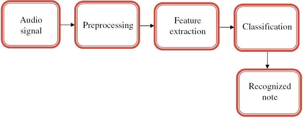
Block Diagram of the Proposed Method.
There are three overall processing stages in our projected algorithm: preprocessing, feature processing, and classification.
4.1 Preprocessing
The primary stage in musical note recognition is to capture the analog input signal and change it to digital form. Filtering is used to eradicate unwanted frequencies. Median filter replaces each value of a signal using the median of the neighborhood entries. Median filters are quite popular because, for convinced kinds of random noise, they give tremendous noise reduction capabilities, with significantly less blurring than linear smoothing filters of similar size [13].
Median filters are chiefly effective in the availability of impulse noise, which is known as salt-and-pepper noise. The median E of a set of values is such that half the values in the set is less than or equal to E and half is greater than or equal to E. To achieve median filtering at a point in an image, first sort the values in question and its neighbors, regulate their median, and assign this value to that entry.
We undertake that an input signal v(g) is the summation of an audio signal m(g) and a transient noise signal t(g).
The transient noise randomly happens in time and has a time-varying unknown impulse response and variance.
where Un is the nth transient noise and Pn(g) and qn(g) are the impulse response and amplitude, respectively.
A comparatively easy manner to eliminate transient noise is to implement a time-domain median filter. Median filter efficiently eliminates transient noise while conserving the slowly varying constituent in the input signal. In other aspects, the slowly varying constituent of anticipated speech remains in the output of the median filter. Furthermore, the median filter is informal to apply, as it does not need any predefined threshold. Although the median filter is operative for eradicating transient noise, it may also distort the distinguishing of anticipated speech but eradicating the fast varying constituent. Consequently, the filter should be implemented only to transient noise presence region to diminish the speech distortion issue.
where medr[v(g)] describes the median filtering operator of that output, which is the median value of input samples from v(g−r) to v(g+r). The length of the median filter 2r+1 should be long adequate to cover the length of transient noise. DU(g) denotes the detection signal of transient noise presence that becomes one if the noise exists and vice versa.
4.2 Feature Extraction
The filtered signal is then forwarded to the feature abstraction stage. In the feature extraction stage, numerous characteristic features are extracted from different music genres. The mid-level representations comprising hundreds or thousands of values designed at discrete time intervals are compressed into around assured characteristic features for each note (or for each time interval if we are using frame-based features). After this stage, each observation from a class is characterized as a point in a space with a restricted number of dimensions [4].
4.2.1 RP
In a linear prediction investigation, each sample is predicted as a linear amalgamation of past L samples. According to this model, the gth sample of speech signal can be approached by a linear weighted sum of L previous samples. Let us describe the prediction error F(g) as the difference within speech signal sample Rk(g) and its predicted value
where p is the order of prediction and dr, 1≤r≤L is the set of real constants.
Energy in the prediction error signal is diminished to regulate the weights known as the LP coefficients (LPCs). The difference within the actual value and the predicted value is known as the prediction error signal or the LP residual. The LP residual F(g) is given by
where Rk(g) is the actual value and
The RP is well defined as the cosine of the phase performance of the analytic signal resulting from the LP residual of a speech signal. Henceforth, we suggest using the phase of the analytic signal resulting from the LP residual. The analytic signal Fd(g) consistent with F(g) is assumed by
where Fn(g) is Hilbert transform of Fn(g) and Fr(g)=IFT[Qn(θ)].
Where
where Q(θ) is the Fourier transform of F(g) and IFT represents the inverse Fourier transform. The magnitude of the analytic signal Fd(g) is specified by
The cosine of the phase of the analytic signal Fd(g) is specified by
where Re(Fd(g)) is the real part of F(g).
4.2.2 MFCC
MFCC is the way of on behalf of the spectral data of a sound in compact form. There is no standard number of MFCC coefficients for distinguishing the sound in any literature. Here, we carried out the experimentation on MFCC to finalize the number of coefficients. MFCC coefficients are adequate to distinguish the instruments. MFCC features are generally found in numerous literature for musical note recognition. The algorithm for receiving MFCC feature is assumed below.
4.2.2.1 Framing
The primary step is framing. The signal is split up into frames characteristically with the length of 10–30 ms (here, frame size=5, frame duration=25 s, and frame shift=10). The frame length is important as tradeoff between time and frequency resolution. The frames overlay each other characteristically by 25%–70% of their own length.
4.2.2.2 Windowing
After the signal is split up into frames, each frame is burgeoned by a window function. For a good window function, the main lobe should be narrow and the side lobe should be low. A smooth tapering contemporaneous at the edges is anticipated to diminish discontinuities. Hamming window is used to eradicate end effects. Hamming window (G[g]) is well defined as
4.2.2.3 Discrete Cosine Transform
The third step is to take discrete cosine transform of each frame.
4.2.2.4 Mel Frequency Warping
The mel scale is based on pitch perception and uses triangular-shaped filter. The scale is roughly linear below 1000 Hz and nonlinear (logarithmic) after 1000 Hz.
4.2.2.5 Log Compression and Discrete Cosine Transforming
The last step is compress the spectral amplitude by considering log and discrete cosine transform. This provides us cepstral coefficient. By spectral smoothing, the MFCC coefficient is computed.
4.3 Music Genre Classification
The extracted features are then promoted to the classification stage, where musical notes are recognized by the OBNN algorithm. In the proposed OBNN, the interconnection weights of the ANN is optimized with the help of the CS optimization method.
4.3.1 ANNs
ANNs are one among the most powerful modeling methods presently being used in numerous fields of engineering. ANNs offer better data fitting skill for complex procedures with numerous nonlinearity and interactions. However, ANN-based modeling is more complex, as frequent decisions associated with ANN architectural and training parameters have to be made.
Among the numerous kinds of ANNs, the FFNN is one among the most popular due to their simplicity and powerful nonlinear modeling ability. The FFNN is a nonlinear mapping scheme collected of numerous neurons (as basic processing units) that are grouped into at least three layers: input, hidden, and output layers. The input neurons are used to feed the ANN with the input information. Through neurons interconnections, each input information is handled with weights to be used in the hidden layer.
The number of nodes in the hidden layer depends on the problem complexity (here, input neuron: 2, hidden neuron: 10, and output neuron: 6). Each hidden node and output node implement a sigmoid function to its net input. It is incessant, monotonically increasing, invertible, and everywhere differentiable function. Training set comprises a group of input output patterns that are used to train the network. Testing set comprises an assortment of input output patterns that are used to access network performance. Learning rate is used to group the rate of weight alterations in the time of network training. The back-propagation algorithm trains a provided feed-forward multiplayer NN for a given group of input pattern with known classifications. When each entry of the sample set is accessible to the network, the network observes its output response to the sample input associated with the known and desired outputs and the error value is considered. Based on the error, the connection weights are accustomed. The back-propagation algorithm is based on the Widrow-Hoff delta learning rule in that the weight adjustment is done via mean square error of the output response to the sample input. The group of these sample patterns is repeatedly offered to the network until the error value is diminished.
The back-propagation algorithm steps are as follows:
Initialize the weight value and provide the random number between 0 and 1 to all the weight values.
Input the samples and stipulate the output layer neuron’s expectations.
Compute the actual output of every layer neuron in sequence.
Adjust the weight value, starting from the output layer to the hidden layer progressively.
Return to step 2. The network study is determined in less than a given error.
4.3.2 Cuckoo Search (CS) Optimization Technique
CS is used to resolve optimization issues that are a metaheuristic algorithm, industrialized by “Xin-She Yang” that is based on the manner of the cuckoo species with the amalgamation of Lévy flight behavior of some birds and fruit flies. The motivation behind evolving the CS algorithm is the invasive reproductive approach and the obligate brood parasitism of some cuckoo species by laying their eggs in the nest of host birds. Some female cuckoos such Guira and Ani can copy the patterns and colors of a few preferred host species. This duplicate power is used to upsurge the hatching probability that brings their subsequent generation. The cuckoo has an amazing timing of laying eggs. Parasitic cuckoos used to pick a nest where the host birds lay their own eggs, and it takes less time to hatch cuckoo’s egg than the host bird’s eggs. After hatching the first egg, the chief instinct action is to throw out the host eggs or to propel the eggs out of the nest to confirm the food from the host bird.
An arbitrarily distributed initial population of host nest is produced and then the population of solutions is subjected to recurrent cycles of the search procedure of the cuckoo birds to lay an egg. The cuckoo randomly selects the host nest position to lay an egg by Lévy flights random-walk and is assumed in subsequent equation:
where
ρ is constant (1≤ρ≤3), Mst is the step size, t is the current generation number, and β is the random number generated between [−1, 1].
The step size is intended by the subsequent equation:
s, n ∈ {1, 2, …, u}, and t∈{1, 2, …, v} are randomly chosen indexes; v is the number of parameters to be optimized, and u is the total population of host nest.
The host bird recognizes the alien egg with the probability value linked to that quality of an egg using the subsequent equation:
where s is the fitness value of the solution.
The egg grows up and stays alive for the subsequent generation based on the fitness function and is represented as
where zsmin and zsmax are the minimum and maximum limits of the parameter to be optimized.
4.3.3 OBNN Algorithm
The CS begins with selecting a random initial population, which is the basis of the optimization algorithm. It frequently comprises three steps for procedure. First, select the best source from the utmost appropriate nests or solutions. The host eggs must be substituted by novel results or cuckoo eggs must be created based on randomization via Lévy flights globally (exploration). Identify few cuckoo eggs by the host birds and change it rendering to the amount of the local random walks (exploitation). There are numerous steps that must be shadowed at the time of each cycle. They are the initialization of appropriate nest or solution, fixing the present host nests, and the egg laid using a cuckoo is discovered by the host bird with a probability pa ε [0, 1].
In the projected CS back-propagation algorithm, each best nest embodies a possible result [i.e. the weight space and the conforming biases for back-propagation NN (BPNN) optimization in this paper]. The weight optimization issue and the size of population signify the quality of the result. In the first epoch, the best weights and biases are primed with CS and then these weights are agreed to the BPNN. The weights in BPNN are considered and associated with the best result in the backward direction. In the subsequent cycle, CS will update the weights with the best possible result and CS will continue searching for the best weights until the last cycle/epoch of the network is extended or either the MSE is attained.
The pseudo code of the suggested CS back-propagation algorithm is
| Step 1: Using CS first initializes and sends the suitable weights to BPNN |
| Step 2: Then the training data must be loaded |
| Step 3: While MSE<stopping criteria |
| Step 4: Select all cuckoo nests |
| Step 5: Pass the cuckoo nests as weights to network |
| Step 6: The weights initialized must besend to the network using Feed forward technique |
| Step 7: The error obtained must be send back |
| Step 8: This process is continued until the network gets converged |
| End While |
5 Results and Discussion
All the programs are developed using MATLAB 7.01. The system configuration is Pentium IV processor with 3.2 GHz speed and 1 GB RAM. Different test cases are carried out to show the efficiency of the proposed CSA and hybrid methodology, which are given below.
A database of musical notes of the musician is constructed using various music genres such as blues, electronic, folk country, jazz, pop, and rock. The fundamental frequency of the sample are calculated during preprocessing and then its features are extracted and given as the input to the NN.
To give a comprehensive view of the results, we use four frame-wise evaluation metrics for binary classification: accuracy, recall/sensitivity, and specificity. These metrics can be represented in terms of the number of true positives (TP; the method says it is positive and ground truth agrees), true negatives (TN; the method says it is negative and ground truth agrees), false positives (FP; the method says it is positive and ground truth disagrees), and false negatives (FN; the method says it is negative and ground truth disagrees).
The various performance measures used for the effective identification of musical notes are accuracy, sensitivity, and specificity.
Sensitivity (SN): Statistical measure of performance of the classifier to detect musical notes correctly.
Sensitivity=(Number of correctly detected music)/(Total number of algorithm positive outcomes)
Specificity (SP): Statistical measure of performance of the classifier to detect musical notes wrongly.
Specificity=(Number of wrongly detected music)/(Total number of algorithm negative outcomes)
Accuracy=(Number of correctly detected musical notes)+(Correctly normal states)/(Total number of cases)
In musical note recognition, five different types of music were identified. They are blues, electronic, folk country, jazz, pop, and rock. Table 1 illustrates the accuracy comparison result between the proposed OBNN and existing method effectiveness in detecting music. The existing method’s accuracy values obtained for various music genres are less, whereas the OBNN system achieves high values. Therefore, our proposed method is more effective in identifying music accurately.
Accuracy Evaluation Results between NN, GMM-UBM, and OBNN.
| Music genres | Accuracy | ||
|---|---|---|---|
| NN | GMM-UBM | OBNN | |
| Blues | 90.93611 | 89.67238 | 91.90193 |
| Electronic | 88.85587 | 89.263 | 90.63893 |
| Folk country | 72.51114 | 70.23347 | 81.87221 |
| Jazz | 64.78455 | 69.22174 | 74.07132 |
| Pop | 87.44428 | 85.6734 | 91.23328 |
| Rock | 68.42496 | 70.23674 | 73.84844 |
The sensitivity evaluation results of different music genres are given in Table 2. The existing method’s sensitivity values obtained for various music genres are also not up to the mark when compared to the proposed method, thus showing effectiveness to detect music correctly.
Sensitivity Evaluation Results between NN, GMM-UBM, and OBNN.
| Music genres | Sensitivity | ||
|---|---|---|---|
| NN | GMM-UBM | OBNN | |
| Blues | 0.241667 | 0.20784 | 0.275 |
| Electronic | 0.40708 | 0.37473 | 0.265487 |
| Folk country | 0.635135 | 0.587894 | 0.391892 |
| Jazz | 0.840125 | 0.6125 | 0.752351 |
| Pop | 0.318966 | 0.083466 | 0.068966 |
| Rock | 0.566292 | 0.538392 | 0.65618 |
The specificity evaluation results of different music genres are given in Table 3. The existing method’s specificity values obtained for various music genres are also lesser than the proposed OBNN. Thus, our proposed method is more effective to detect music correctly.
Specificity Evaluation Results between NN, GMM-UBM, and OBNN.
| Music genres | Specificity | ||
|---|---|---|---|
| NN | GMM-UBM | OBNN | |
| Blues | 0.974715 | 0.957828 | 0.982055 |
| Electronic | 0.932685 | 0.924263 | 0.965126 |
| Folk country | 0.742883 | 0.83553 | 0.903025 |
| Jazz | 0.588121 | 0.83646 | 0.737098 |
| Pop | 0.926829 | 0.983263 | 0.99187 |
| Rock | 0.914474 | 0.87346 | 0.899123 |
The accuracy comparison of the proposed OBNN and existing NN and Gaussian mixture model-universal background model (GMM-UBM) methods for identifying different music genres is shown in Figure 2. The accuracy of our proposed method is high compared to the existing methods. It represents that OBNN correctly classifies the music.

Accuracy Comparisons of the Proposed and Existing Methods.
Figure 3 illustrates the sensitivity comparison of the proposed and existing methods. The sensitivity of the proposed method is low compared to the existing method. It indicates that it effectively identifies the music.

Sensitivity comparisons of the proposed and Existing Methods.
Figure 4 illustrates the specificity comparison of the proposed and existing methods. The specificity of the proposed method is high compared to the existing method. It indicates that it effectively discovers different music signals.

Specificity Comparisons of the Proposed and Existing Methods.
6 Conclusion
In this study, musical notes were accurately classified. Issues such as noise, variable amplitude, and tone color were present on the audio files conforming to the data set, although it was observed that the NN was robust enough to discriminate these problems. The system was able to recognize the fundamental note of the input chord, demonstrating the validity of the proposed approach and the robustness of the NN to noisy signals.
Bibliography
[1] D. G. Bhalke, C. B. Rama Rao and D. S. Bormane, Dynamic time warping technique for musical instrument recognition for isolated notes, in: Proceedings of International Conference on Emerging Trends in Electrical and Computer Technology (ICETECT), 2011.10.1109/ICETECT.2011.5760221Search in Google Scholar
[2] S. Chanda, D. Das, U. Pal and F. Kimura, Offline hand-written musical symbol recognition, in: Proceedings of International Conference on Frontiers in Handwriting Recognition, 2014.10.1109/ICFHR.2014.74Search in Google Scholar
[3] J. de Jesus Guerrero-Turrubiates, S. E. Gonzalez-Reyna, S. E. Ledesma-Orozco and J. G. Avina-Cervantes, Pitch Estimation for Musical Note Recognition Using Artificial Neural Networks, 2014.10.1109/CONIELECOMP.2014.6808567Search in Google Scholar
[4] A. Gordo, A. Forne and E. Valveny, Writer identification in handwritten musical scores with bags of notes, Pattern Recog.46 (2013), 1337–1345.10.1016/j.patcog.2012.10.013Search in Google Scholar
[5] S. Hsieh, M. Hornberger, O. Piguet, and J. R. Hodges, Brain correlates of musical and facial emotion recognition: evidence from the dementias, Neuropsychological50 (2012) 1814–1822.10.1016/j.neuropsychologia.2012.04.006Search in Google Scholar PubMed
[6] Ş. Kolozali, M. Barthet, G. Fazekas, and M. Sandler, Automatic ontology generation for musical instruments based on audio analysis, IEEE Trans. Audio Speech Lang. Process.21 (2013), 2207–2220.10.1109/TASL.2013.2263801Search in Google Scholar
[7] T. León and V. Liern, A fuzzy framework to explain musical tuning in practice, Fuzzy Sets Syst.214 (2013), 51–64.10.1016/j.fss.2011.08.007Search in Google Scholar
[8] J. B. Prince and P. Q. Pfordresher, The role of pitch and temporal diversity in the perception and production of musical sequences, Acta Psychol.141 (2012), 184–198.10.1016/j.actpsy.2012.07.013Search in Google Scholar PubMed
[9] Y. Sazaki, R. Ayuni and S. Kom, Musical Note Recognition Using Minimum Spanning Tree Algorithm, 2014.10.1109/TSSA.2014.7065919Search in Google Scholar
[10] P. Taweewat and C. Wutiwiwatchai, Musical pitch estimation using a supervised single hidden layer feed forward neural network, Expert Syst. Appl.40 (2013), 575–589.10.1016/j.eswa.2012.07.063Search in Google Scholar
[11] E. Vincent, N. Bertin and R. Badeau, Adaptive harmonic spectral decomposition for multiple pitch estimation, IEEE Trans. Audio Speech Lang. Process.18 (2010), 528–537.10.1109/TASL.2009.2034186Search in Google Scholar
[12] Z. Wei and C. Wu, Mechanical systems and signal processing an information processing method for acoustic emission signal inspired from musical staff, Mech. Syst. Signal Process.66 (2016) 388–398.10.1016/j.ymssp.2015.06.015Search in Google Scholar
[13] J. Wu, E. Vincent, S. A. Raczynski, T. Nishimoto, N. Ono and S. Sagayama, Polyphonic pitch estimation and instrument identification by joint modelling of sustained and attack sounds, IEEE J. Select. Top. Signal Process.5 (2011).10.1109/JSTSP.2011.2158064Search in Google Scholar
[14] J. X. Zhang, M. G. Christensen, S. H. Jensen and M. Moonen, An iterative subspace-based multi-pitch estimation algorithm, Signal Process91 (2011), 150–154.10.1016/j.sigpro.2010.06.010Search in Google Scholar
©2019 Walter de Gruyter GmbH, Berlin/Boston
This article is distributed under the terms of the Creative Commons Attribution Non-Commercial License, which permits unrestricted non-commercial use, distribution, and reproduction in any medium, provided the original work is properly cited.
Articles in the same Issue
- Frontmatter
- An Effective Technique to Track Objects with the Aid of Rough Set Theory and Evolutionary Programming
- A Novel Word Clustering and Cluster Merging Technique for Named Entity Recognition
- Simulation-Based Analysis of Intelligent Maintenance Systems and Spare Parts Supply Chains Integration
- Retinal Fundus Image for Glaucoma Detection: A Review and Study
- Task Reallocating for Responding to Design Change in Complex Product Design
- Fuzzy Mutual Information-Based Intraslice Grouped Ray Casting
- An Efficient Compound Image Compression Using Optimal Discrete Wavelet Transform and Run Length Encoding Techniques
- A Fast Internal Wave Detection Method Based on PCANet for Ocean Monitoring
- A Wheelchair Control System Using Human-Machine Interaction: Single-Modal and Multimodal Approaches
- Design of Optimized Multiobjective Function for Bipedal Locomotion Based on Energy and Stability
- Hybridization of Genetic and Group Search Optimization Algorithm for Deadline-Constrained Task Scheduling Approach
- An Effective Optimization-Based Neural Network for Musical Note Recognition