Causal additive models with smooth backfitting
-
Asger B. Morville


Abstract
A fully nonparametric approach to learning causal structures from observational data is proposed. The method is described in the setting of additive structural equation models with a link to causal inference. The estimation procedure of the additive structural equation functions is based on a novel application of the smooth backfitting (SBF) approach. The flexibility of the nonparametric procedure results in strong theoretical properties in the estimation of the variable ordering. It is shown that under mild conditions, the ordering estimate is consistent. Through simulations, it is demonstrated that our method is superior to the state-of-the-art approaches to causal learning. In particular, the SBF approach shows robustness when the noise is heteroscedastic.
1 Introduction
In statistical analyses, one is often interested in finding causal relationships among observed variables. In traditional statistical models, one is typically not able to infer causal structures using only the joint distribution of the variables. This is because there are often multiple data generating mechanisms that lead to an identical joint distribution. One way of finding causal links among variables is to construct interventional experiments. This technique is used in contexts such as clinical trials and A/B-testing on user platforms and is considered the gold standard for finding causal relationships. In many cases, however, such interventional experiments are expensive to carry out. Furthermore, they may be infeasible to conduct from an ethical point of view. As such, for observational data, the conventional practice is to simply avoid causal conclusions, making correct probabilistic statements such as “Variable
An approach to causal discovery with observational data that has drawn recent attention is to formulate a causal model where each joint distribution in the model is associated with a unique data generating mechanism. In this approach, a causal model represents a family of data generating mechanisms and each data generating mechanism corresponds to a directed acyclic graph (DAG) with a set of structural equations linking the “cause” and “effect” variables in the DAG. By estimating the underlying DAG (and the associated set of structural equations) from observational data, one can deduce legitimate causal relationships among variables. This approach is recently studied by Peters et al. [1], who has shown that the underlying DAG is identifiable if the associated structural equations are non-linear in the variables and the additive error terms have a density with non-zero support on the real line. It is further developed by Bühlmann et al. [2], where the structural equations are assumed to be additive in the variables as well as in the error terms. Here, the errors are assumed to follow a Gaussian distribution.
The objective of this article is to propose a new nonparametric approach to the estimation of the underlying DAG for
We show that our approach based on the SBF is consistent under weak conditions when estimating the variable ordering. Furthermore, our numerical results demonstrate that it is superior to the state-of-the-art algorithms for causal discovery. We also extend the model to incorporate heterogeneous variance, and we provide the conditions under which the ordering estimator is consistent in this setting. Importantly, we note that the theoretical developments in the study of Bühlmann et al. [2] do not address the case of heterogeneous variance. Research focusing on this setting has primarily been conducted in simple two-variable set ups, see, e.g., [12].
There exists a large body of research regarding the estimation of DAG structures from observational data. Constraint-based methods directly make a set of conditional independence statements through statistical tests. The methods then identify a set of DAGs consistent with this set of conditional independence statements, see, e.g., [13] and [14]. Methods that are more related to our approach construct a score for each possible DAG structure. The DAG that maximizes the score function is then found by traversing through the space of DAGs in a computationally feasible way, see, e.g., [15–17]. Specifically, the general ordering-based search method of Wang et al. [17] has received much attention in the DAG estimation literature. This is due to the fact that once an ordering among the variables has been established, finding the best scoring DAG consistent with this ordering reduces to simple variable selection, see, e.g., [2,18,19]. Other alternative approaches to DAG estimation include gradient-based optimization techniques [20,21] and reinforcement learning [19,22].
DAG estimation within causal models from observational data is performed in models where the underlying DAG is identifiable. Examples include the nonlinear Gaussian model of Peters et al. [1], the linear non-Gaussian model of Shimizu et al. [23], the post-nonlinear model of Zhang and Hyvärinen [24] and the equal-variance linear Gaussian model of Peters et al. [25]. We refer to Glymour et al. [26] for a more comprehensive review of causal discovery algorithms.
Throughout the article, we consider a random vector
We proceed as follows. In Section 2, we formulate an additive SEM along with some basic assumptions that make the model identifiable and then describe a general estimation procedure of recovering the underlying DAG. In Section 3, we present our proposal of estimating a true ordering of variables based on the SBF technique together with its supporting theory. Section 4 is devoted to extending the method and theory to the case where the additive error terms in the SEM have heterogeneous variances depending on parent variables. In Sections 5 and 6, we report the results of numerical studies demonstrating the efficiency of our proposal and conclude in Section 7 with some discussion. All technical proofs for the theoretical results presented in this article and additional numerical results are deferred to the Appendix.
2 Problem set-up
2.1 The additive structural equation family
We define a general SEM over
and
We define the additive family
where the errors
Assumption 1
The functions
Assumption 2
The functions
Assumption 3
For any
exist. In addition, the marginal density
Assumption 4
The variances of the noise variables are strictly positive, i.e.
Note that the technical condition in Assumption 3 is met when the component functions
Remark 1
An SEM
In Section 2.2, we describe a general estimation technique that is employed to estimate the underlying graph
2.2 General estimation procedure
We fix an SEM
In words,
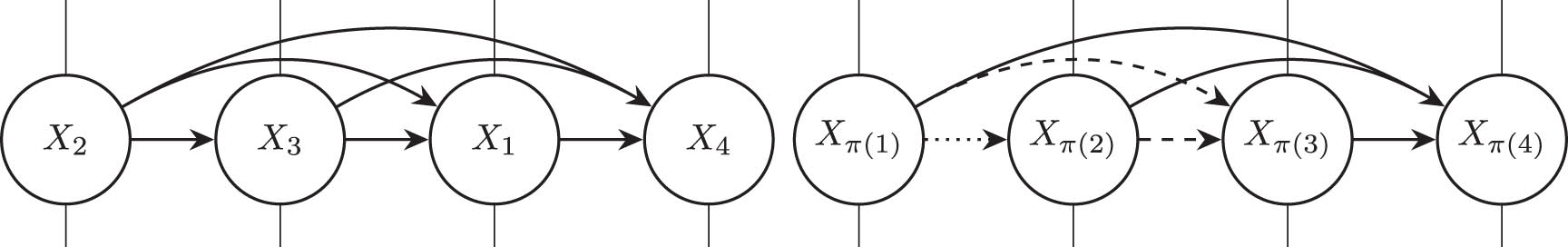
The left panel illustrates the fully connected graph
We define the functions
The subscript
The general estimation procedure of
In Section 2.3, we will show why this implies
2.3 Ordering identification and graph pruning
With
where
Proposition 1
Let
where
In the following, we apply Proposition 1 to show that for a true ordering
Proposition 2
Let
We define
If two measures
Proposition 3
Let
The following proposition is a consequence of Proposition 3 and a modification of Corollary 31 in the study of Peters et al. [1].
Proposition 4
For any
Proposition 4 gives a way of separating correct orderings from incorrect orderings in the sense that
Proposition 5
Fix an SEM
In particular,
Combining Propositions 2–5, we obtain that
Assume now that
3 Estimation of a true ordering
In this section, we detail how a true ordering
With these estimates, we may construct the estimator of a true ordering
With the ordering
3.1 SBF
We describe the SBF technique in a general regression setting. Let
where
the projection of
Assume now that we observe iid copies
We define first the normalized kernel weight functions
Here, the function
From the marginal density estimators
We then define the NW-SBF estimator of
The existence, uniqueness, and consistency of
Assumption (B1)
The joint density
Assumption (B2)
The marginal regression functions
Assumption (B3)
Assumption (C1)
The baseline kernel function
Assumption (C2)
The bandwidths satisfy that
In the SBF literature, it is typically assumed that
Proposition 6
Under the conditions in Assumptions (B1), (C1), and (C2), there exist a unique solution
There is a geometric interpretation of the SBF estimator
3.2 Estimation of a true ordering
In this subsection, we describe an ordering estimator as prescribed at (9) and show that it is a true ordering with probability tending to one under weak conditions. Recall that the SBF technique is applicable to compactly supported covariates. Since the variables in
by the SBF method. To this end, we construct the random variables
and we note that
where
Using these observations, we obtain the ordering estimator by applying the SBF method described in Section 3.1 to estimating
for each
With the filtered observations for the response
where
We include the superscript
We note that, for each
Proposition 7
Let
A consequence of Proposition 7 is that we need only Assumptions (C1) and (C2) for the uniform convergence result in Proposition 6 with
Proposition 8
Assume that
According to our discussion in Section 2.3, the key element for the consistency of
Theorem 1
Assume that
(i) Case 1 (true orderings):
Suppose that
(ii) Case 2 (non-true orderings):
For any
Both cases in Theorem 1 are the consequences of the second part of Proposition 6 regarding the uniform convergence of the SBF estimator on compact domains. Theorem 1, in turn, implies that we can construct a compact set
Theorem 2
Assume that
We note that the conditions for Thorem 2 are weaker than those for Theorem 1 in Bühlmann et al. [2], which in part relies on an empirical process argument.
In the practical implementation of
4 Ordering estimation with heterogeneous noise
In this section, we explore the setting where the noise is heterogeneous. In Section 4.1, we introduce a heterogeneous structural equation family which will serve as the statistical model for the observations. In Section 4.2, we state an identifiability result regarding the variable ordering. Finally, in Section 4.3, we present a consistency result for the ordering estimator which is valid under some extra conditions. We note that most of the theory here mirrors that of the previous sections, with a few exceptions that we highlight. In particular, the uniform convergence result of Proposition 6, which is the key theorem underpinning the results of Section 3.2, does not rely on the homogeneity of the error variances.
4.1 Model set-up
We generalize the structural equation family
In the model (21), the errors
Assumption 4’
The functions
It follows that
4.2 Identifiability of the true variable ordering
In a similar manner as in the case with homogeneous noise, for a fixed
The associated SEM
Proposition 9
If
The proof is based on an identifiability result from the study of Immer et al. [12]. The moral of Proposition 9 is that only in pathological cases we have
Proposition 10
Fix an SEM
In particular,
In a similar way as to how it was shown for the homogeneous variance case, we have that the ordering
4.3 Consistency of the ordering estimator
We do not have access to the functions
We consider an alternative ordering
The estimated ordering
Theorem 3
Assume that
As shown in Proposition 9, requiring
5 Simulation study
The structure of this section is as follows. Section 5.1 details the simulation setup of the subsequent numerical experiments. In Section 5.2, we compare our proposed SBF estimator against some of the state-of-the-art algorithms introduced in Section 1 for recovering the variable ordering. In Section 5.3, we include the variable selection step in the comparison, where the goal is the recovery of the underlying DAG, not only of the variable ordering. Section 5.4 contains some remarks on the comparison of different methods.
Throughout all the experiments in this section, we let the number of observed variables
5.1 Simulation set-up
When evaluating the quality of the variable ordering estimate we use the structural intervention distance (SID) introduced in the study of Peters and Bühlmann [29]. This is a pre-distance measure over DAGs which has the property that if
Data generation. When generating a graph consistent with this ordering, there are a total number of
We also include the results for the case where the noise is heterogeneous. In this case, we simulate data according to the model in (21). As in the homogeneous variance case, the functions
Estimation of variable ordering and underlying graphs. For the estimation of the variable ordering, by the estimator defined in (20), we need to cycle through all the possible
For the implementation of the SBF optimization loop, we transform the data such that each variable lies within the unit interval. The fitted functions are then scaled back to the original position after estimation is done. When performing variable selection for the graph pruning step (see the last part of Section 2.3) we apply the functional lasso-method described in Lee et al. [32] which is a generalization of the lasso method of Tibshirani [33] to the SBF setting. Finally, for the SBF method the Epanechnikov kernel is used as the baseline kernel function and the bandwidth parameter is chosen according to Silverman’s rule of thumb in each dimension, see Shimizu et al. [34].
Other methods in comparison. We compare our method with the methods, CAM in Bühlmann et al. [2], SCORE in Rolland [18], LiNGAM in the study of Shimizu et al. [35], RESIT in the study of Peters et al. [1] and GES in the study of Chickering [16]. Note that all these methods except the GES consist of first establishing an estimate of true variable ordering and then performing variable selection. The GES does not perform the estimation of variable ordering, but instead directly estimates the Markov equivalence class of the underlying DAG.
The CAM is fitted in R using the CAM-library provided by the authors. The SCORE is fitted in Python using the code made publicly available on the authors’ Github page. The LiNGAM and RESIT are fitted using the Causal Discovery library provided by Ikeuchi et al. [36]. The method of GES is fitted using the ges package in Python.
We note that for variable selection, the CAM and SCORE both rely on the gam-function from the mgcv-library in R, see Wood [37]. We remove the edges that correspond to
We note that comparing the implied ordering estimates of the GES with the other methods in terms of the SID to the true underlying DAG can be slightly misleading. This is because the estimates by the GES are already pruned, and thus, we expect these estimates to be further from the true orderings than the ordering estimates provided by the other methods.
5.2 Recovery of the variable ordering
We set the probability
SID from the true ordering to the estimated ordering when the underlying graph is sparse
| Homogeneous variance | Heterogeneous variance | |||||
|---|---|---|---|---|---|---|
| Method |
|
|
|
|
|
|
| SBF (our method) |
3.2
|
0.4
|
0.0
|
5.5
|
|
0.0
|
| CAM | 4.9
|
0.4
|
0.0
|
7.1
|
0.8
|
0.1
|
| SCORE | 6.7
|
3.5
|
1.4
|
5.9
|
3.0
|
1.2
|
| LiNGAM | 31.1
|
33.1
|
36.0
|
34.5
|
34.3
|
34.1
|
| RESIT | 20.6
|
17.8
|
11.1
|
27.4
|
27.6
|
29.1
|
| GES* | 29.2
|
25.5
|
22.3
|
31.5
|
29.1
|
25.6
|
The smallest values among different methods are bold faced.
We see that the SBF approach performs well in establishing a correct variable ordering in this setting. Only in the case with heterogeneous variance and sample size being
We note that when the sample size
5.3 Recovery of the underlying graph
In this subsection, we set out to do a complete recovery of the underlying graph rather than only estimating the variable ordering. To encompass different settings, we shall in our experiment report results for both the settings where the underlying graph is sparse and for the setting where it is dense. In the sparse setting, we set the probability of including each of the possible
The results can be seen in Table 2 for the sparse graph setting, and in Table 3 for the dense setting. The SBF method clearly demonstrates good performance throughout the various settings, where it shows large reductions in the distance to the true underlying graph with respect to both the SID and SHD-measure. We glean from Tables 2 and 3 that it is generally harder to estimate the graph in the dense setting, as the graph estimates in general have greater distances to the true underlying graph in comparison to the sparse setting. Only in the sparse setting with homogeneous variance and sample size
SID and SHD from the true underlying graph to the estimated graph in the sparse setting
| Homogeneous variance | Heterogeneous variance | |||||||
|---|---|---|---|---|---|---|---|---|
| SID | SHD | SID | SHD | |||||
| Method |
|
|
|
|
|
|
|
|
| SBF (our method) |
|
6.5
|
|
|
6.5
|
5.4
|
5.3
|
2.3
|
| CAM | 16.9
|
6.0
|
6.6
|
2.7
|
18.8
|
7.2
|
6.8
|
2.9
|
| SCORE | 19.1
|
10.8
|
7.3
|
3.9
|
19.9
|
11.2
|
7.3
|
4.1
|
| LiNGAM | 30.6
|
31.7
|
10.0
|
10.1
|
29.4
|
30.3
|
9.8
|
10.0
|
| RESIT | 28.6
|
31.1
|
16.3
|
17.6
|
28.3
|
29.6
|
16.3
|
17.0
|
| GES | 27.7
|
25.8
|
12.2
|
10.7
|
25.7
|
25.5
|
11.3
|
10.3
|
The smallest values among different methods are bold faced.
SID and SHD from the true underlying graph to the estimated graph in the dense setting
| Homogeneous variance | Heterogeneous variance | |||||||
|---|---|---|---|---|---|---|---|---|
| SID | SHD | SID | SHD | |||||
| Method |
|
|
|
|
|
|
|
|
| SBF (our method) |
28.9
|
19.1
|
12.6
|
6.6
|
31.0
|
20.0
|
16.0
|
8.5
|
| CAM | 55.8
|
30.1
|
23.8
|
12.8
|
59.6
|
39.2
|
25.2
|
17.0
|
| SCORE | 56.7
|
35.8
|
24.2
|
14.8
|
58.9
|
41.0
|
25.1
|
17.5
|
| LiNGAM | 74.3
|
74.5
|
30.4
|
29.9
|
75.2
|
75.8
|
30.0
|
30.4
|
| RESIT | 72.9
|
74.1
|
31.9
|
31.6
|
72.7
|
74.6
|
30.6
|
31.9
|
| GES | 72.6
|
73.2
|
31.1
|
31.1
|
73.8
|
73.1
|
30.7
|
30.6
|
The smallest values among different methods are bold faced.
5.4 Some remarks
The simulation results show that the SBF method has the best performance among all, followed by the CAM and SCORE methods. We note that the LINGAM and GES methods do not satisfy the nonlinearity requirement and a natural consequence is that these two methods have poorer performance than the first three. The RESIT method uses an independence testing when identifying the variable ordering. It is seen in the study of Bühlmann et al. [2] that the independence testing is inferior to the general greedy ordering search framework that is used in the CAM and in our method. The SCORE algorithm is developed with the intention of optimizing for the computational speed, and thus it may not beat the existing methods in terms of accuracy. In comparison with the CAM method, our approach of using the functional Lasso in the variable selection step, in particular, turns out to be beneficial. This can be seen by comparing Table 1 with Table 2. In Table 1 where we only estimate the ordering and do not perform graph pruning, we see that the CAM and SBF estimates exhibit a similar performance although the SBF method is better with a slight edge in the
6 Causal pathways for prostate cancer
Identifying causal genes in disease development is crucial for understanding the mechanisms that drive pathological changes. In particular, this may enable early diagnosis, disease prevention, and development of specific gene therapies. It is an active area of research, see, e.g., [38–40].
In the study of Wang et al. [41], the gene expression levels of more than 13,000 mRNA genes were sampled across 125 patients with varying levels of prostate cancer. They identified 20 hub genes that were highly interconnected with other genes. These hub genes were suspected to form a causal pathway for the development of prostate cancer.
The dataset with ID GSE20161 was obtained from NCBI’s Gene Expression Omnibus database. The data were extracted from the database in R using the GEOquery-package by Davis and Meltzer [42] from the Bioconductor website. The GEO database with ID GPL6102 was used to translate the probe IDs to the gene names.
In the study of Wang et al. [41], the specific preprocessing of the data can be found. We standardize the data to have mean zero and variance one. Further, in the SBF estimation scheme, the data are transformed so that the gene expression levels are within the unit interval. The fitted functions and data are then scaled back to the standardized scaling after estimation is done.
In Table 4, the estimated variable ordering before performing variable selection can be seen. This ordering estimate suggests that the CDC2-gene plays the role of the root node, not having any of the other hub genes affecting its value. In contrast, it is seen that CDCA2 is estimated to be the last gene in the ordering. This suggests that performing an intervention on this variable has no effect on the other variables under observation.
Estimated variable ordering by the SBF method before performing variable selection
| Order | Gene | Order | Gene | Order | Gene | Order | Gene |
|---|---|---|---|---|---|---|---|
| 1 | CDC2 | 6 | NCAPG | 11 | ATAD2 | 16 | TOP2A |
| 2 | CCNA2 | 7 | TTK | 12 | MELK | 17 | HJURP |
| 3 | CDCA5 | 8 | CCNB2 | 13 | PLK4 | 18 | Ska1 |
| 4 | ORC1L | 9 | CEP55 | 14 | DTL | 19 | AURKA |
| 5 | KIF15 | 10 | TPX2 | 15 | KIF23 | 20 | CDCA2 |
These are the hub genes suspected to form a causal pathway for the development of prostate cancer. The CDC2 hub-gene is seen to constitute a root node, and according to this estimate modifying the CDC2 would affect other genes downstream.
In addition to estimating the variable ordering, we also perform variable selection to obtain a final graph estimate
After performing variable selection, only 32 edges remained out of the 190 edges in the estimated fully connected DAG. In the following, we develop a measure to gauge the causal strength of each of the 32 included edges. In Figure 2, the final graph estimate
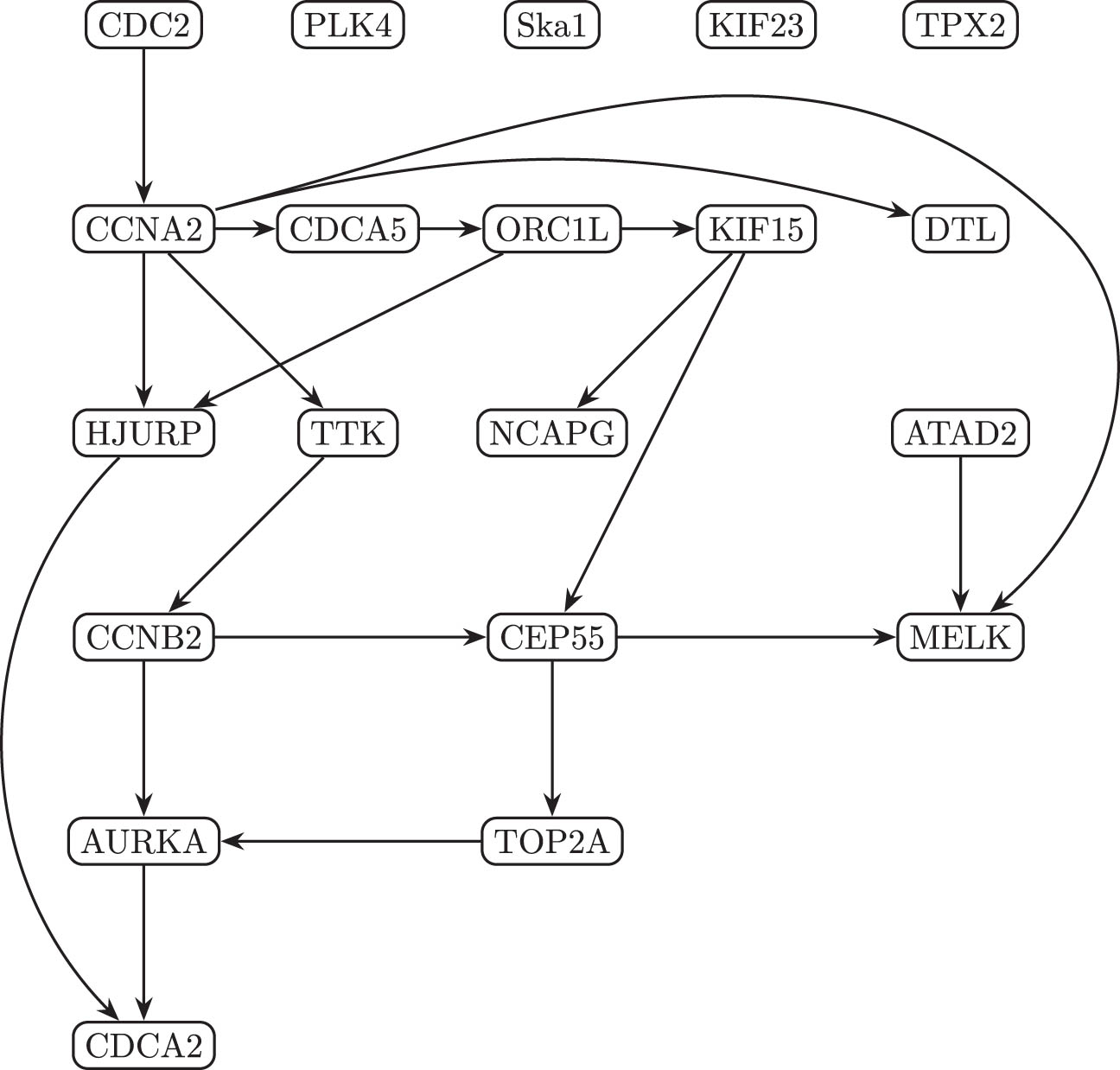
Estimated causal graph
In order to assess the strengths of each of the 32 included edges in
Given that our estimate
In Table 5, the
Strength of the 20 edges associated with the largest causal strengths from the graph
| Parent | Child |
|
Parent | Child |
|
Parent | Child |
|
Parent | Child |
|
|---|---|---|---|---|---|---|---|---|---|---|---|
| CCNA2 | CDCA5 | 3.96 | CCNA2 | MELK | 1.05 | CEP55 | MELK | 0.80 | CCNB2 | CEP55 | 0.73 |
| CDC2 | CCNA2 | 3.21 | CCNA2 | DTL | 1.02 | TTK | CCNB2 | 0.77 | CCNA2 | TTK | 0.72 |
| KIF15 | NCAPG | 1.50 | ATAD2 | MELK | 0.94 | HJURP | CDCA2 | 0.76 | KIF15 | CEP55 | 0.72 |
| ORC1L | KIF15 | 1.23 | CEP55 | TOP2A | 0.93 | CCNA2 | HJURP | 0.74 | TOP2A | AURKA | 0.71 |
| CDCA5 | ORC1L | 1.07 | AURKA | CDCA2 | 0.83 | ORC1L | HJURP | 0.74 | CCNB2 | AURKA | 0.69 |
Finally, we also test the robustness toward the choice of the underlying compact subset
We then investigate how well we recover the relationship
Note that
Consistency of the choice of compact
|
|
0.1 | 0.2 | 0.3 | 0.4 | 0.5 | 0.6 | 0.7 | 0.8 | 0.9 | 1.0 |
|---|---|---|---|---|---|---|---|---|---|---|
|
|
|
|
|
|
|
|
|
0.0098 | 0.0208 | 0.0025 |
7 Conclusion
We applied the non-parametric SBF approach to fitting non-linear SEMs in order to obtain an estimate of the variable ordering. The estimator possesses strong theoretical guarantees of convergence toward the true variable ordering associated with the data compared to existing estimators. Furthermore, it shows strong performance in a simulation setup against the state-of-the-art methods in the field of causal discovery. We also extended the model and estimator to the case where the noise is heterogeneous.
Due to the generality of the SBF estimator, it would be interesting to extend the framework to cases where the observed variables are non-Euclidean. In particular, the setting where the variables are Hilbert-space valued has direct applications to the field of neuroscience. Here, the neuron activity is frequently recorded over time, resulting in function-valued data. Such an extension could provide significant insights into brain function and neural interactions.
The setting where
-
Funding information: This research was supported by the National Research Foundation (NRF) grant funded by the Korea government (MSIP) (No. RS-2024-00338150).
-
Author contributions: Both authors have accepted responsibility for the entire content of this manuscript and consented to its submission to the journal, reviewed all the results, and approved the final version of the manuscript. The study and manuscript have received significant contributions from both authors.
-
Conflict of interest: The authors state no conflict of interest.
-
Data availability statement: Empirical results of the current study can be generated using the code from https://github.com/AsgerMorville/sbf-causal-discovery/. The real world dataset was obtained from NCBI’s Gene Expression Omnibus database with ID GSE20161.
Appendix
A.1 Proof of Proposition 1
For
By this with (2) and (6), we obtain that
Thus,
which shows that
This gives the theorem. To prove the claim, suppose that it is false, i.e., there exists
A.2 Proof of Proposition 2
Fix
for all
For
where the first equality follows from (A3) and the second from (A2).
A.3 Proof of Proposition 3
The density
Here, we have defined
Since the joint density of the variables
for every
is two times differentiable in each argument, and note that the same property can be shown for
and it is therefore enough to show that for any choice of marginalizing covariates
is twice differentiable. This, in turn, holds by Assumption 3.
A.4 Proof of Proposition 4
Fix a variable ordering
that relate
Lemma A1
(Slight modification of Corollary 31 in [1]) Assume that
Assume that the functions
Assume that the functions
A.5 Proof of Proposition 5
For any
where
when
By (A5), we thus have
since the two constant terms cancel out.
A.6 Proof of Proposition 7
The density of
A.7 Proof of Proposition 8
This follows directly from Propositions 7 and 6.
A.8 Proof of Theorem 1
Proof of Case 1: π ∈ Π0
Fix
as proven in Proposition 1, and thus
where for the third equality we have used that
By adding and subtracting
Note that by the law of large numbers, the first term on the right-hand side converges to its expectation,
Both of the last two terms converge to zero, as by Proposition 6, we have
and thus,
This gives that
Proof of Case 2: π ∉ Π0
It is enough to show that for any
Fix
By Hölder’s inequality, the second term on the right-hand side of (A6) is bounded by
Using that the fourth moments are finite, i.e. Assumption 1, we thus obtain
For the first term on the right-hand side of (A6), note that by definition
Let now
If we show that
then we are done. Recall that
and that
It then holds that
where
since
and thus
This gives that
Now, since
This proves (A7) and the second part of the theorem.□
A.9 Proof of Theorem 2
It suffices to prove the following result: there exists a non-trivial compact set
Let
The equality holds by Proposition 5 and the inequality holds by Proposition 4. By the continuity of
Put
Now, by Theorem 1-(i) and the continuous mapping theorem, it holds that, for any
For the limiting values
This completes the proof of (A8).
A.10 Proof of Proposition 9
The proof of Proposition 9 runs along the same lines as the proof of Proposition 4, now using the identifiability result in Theorem 4 of [12].
A.11 Proof of Proposition 10
The proof of Proposition 10 runs along the same lines as the proof of Proposition 5 and thus is omitted here.
A.12 Proof of Theorem 3
Define first
Note that under the hypothesis that
Define
By the continuity of
Put
where
Then, by the inequalities at (A13) and at (A14), we obtain that
where for the second inequality we have used the definition of
We prove the first claim at (A14). Note that
The value of the second term on the right-hand side can be made arbitrarily small for any
Now,
Next, we prove the second part of (A14). By the same argument as in the case
However, here we do not necessarily have
A.13 Proof of Proposition 6
By (15), the SBF estimator
Under Assumptions (B1), (C1) and (C2) there exists a constant
with probability tending to one. The existence of a solution to the backfitting equations in (A15) then follows from Theorem 2.1 in the study of Park [43], see also Theorem 3.4 in the study of Jeon and Park [8].
Now, we prove that, uniformly for
To prove (A16), suppose that the baseline kernel function
Also, we have
where “Leb” denotes the Lebesgue measure on
To show the convergence results in (A18), we observe that
This implies
From this and the facts that
We define now the sqaces
Since
that project functions
Then, from (A16), it can be shown that, uniformly in
where
see, e.g. [3]. It is therefore enough to show
For an element
Consider now the following four claims:
Note that in (A22), we suppress the dependence of
The first and second term, on the RHS are
The first factor in the quantity on the right is
A.14 Proof of (A20)
By ordinary kernel smoothing theory, due to Assumptions (B1)–(B3) and (C1)–(C2),
Letting
where
When
where
A.15 Proof of (A21)
Note that by Lemma A4,
where
A.16 Proof of (A22)
Since
where for each
where
For
where now we have
A.17 Proof of (A23)
Note that by Lemma A5, with probability tending to one it holds that
for some
with probability tending to one. We show that
where
for each
since
A.18 Proof of Lemma A1
Note that the proof of this slightly more general statement is almost identical to the proof of Corollary 31 in [1], but we include it here for completeness. Assume for contradiction that the distribution of
and such that the following holds:
The parents of
The parents of
See Figure A1 for an illustration of this choice of
By a disintegration argument one can show that the conditional distribution
is equal to the distribution on the form
The proof relies on the fact that
Both
By the lemma assumptions,
Now, if
Combining this equation with (A31), and using that
By the chain rule, it follows that
It also follows that
Combining these expressions yield
If
Taking the derivative of this expression with respect to
and this implies that
for some constant
This expression implies
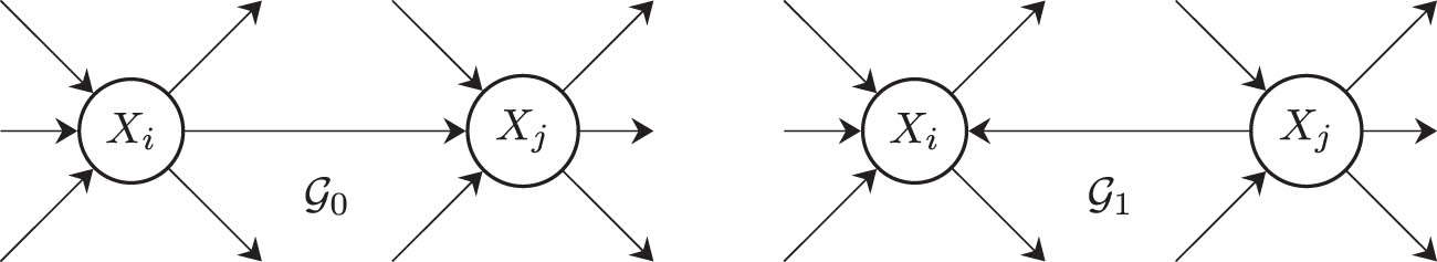
Illustration of the choice of
A.19 Some lemmas from the SBF literature
This section contains lemmas from the theory of SBF that are needed in the proof of Proposition 6. As these lemmas are well known, see, e.g., [3] and [8], the proofs are omitted.
Lemma A2
If
Lemma A3
If
Lemma A4
The sequential projection operator
where each
where
Lemma A5
Under Assumption (B1), for the empirical projection operators
with probability tending to one. Furthermore, for the sequential projection operator
with probability tending to one.
A.20 The role of heterogeneity and non-linearity
To understand the consequences of heterogeneous variance, we will in this section see an example where the estimator in (24) might fail to converge to the true variable ordering. We simulate a two-variable set up, where
where
for various settings of
We require that
It turns out that when we increase
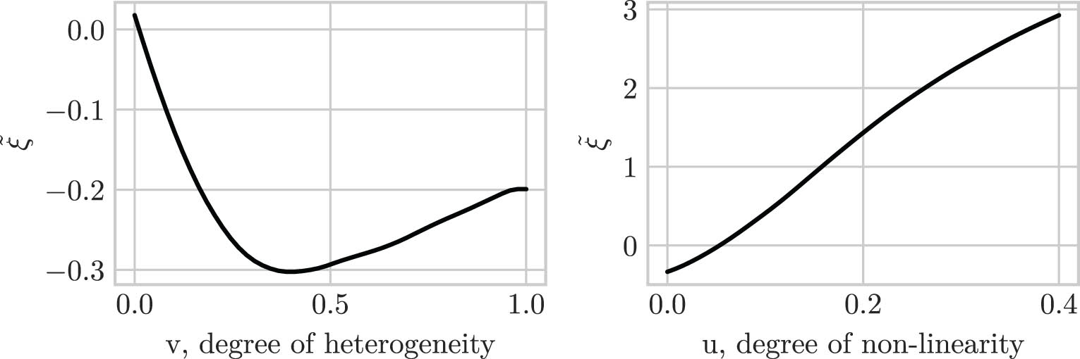
Note however that in this setting the structural function
and where
A.17 Simulation results for large p
We include here the simulation results for the case where
SID and SHD from the true graph to the estimated graph, in the sparse setting (homogeneous error variance) with
| Homogeneous variance | ||||
|---|---|---|---|---|
| SID | SHD | |||
| Method |
|
|
|
|
| SBF (our method) |
25.1
|
17.0
|
13.5
|
4.6
|
| CAM | 59.7
|
25.9
|
23.5
|
11.6
|
| SCORE | 63.7
|
45.5
|
23.6
|
14.4
|
| LiNGAM | 89.0
|
85.7
|
20.3
|
19.8
|
| GES | 90.0
|
80.0
|
33.9
|
27.4
|
A.18 Simulation results for a different choice of bandwidth
Throughout the numerical studies in Sections 5 and 6, we used Silvermans rule of thumb in order to automatically select the bandwidth. Such a particular bandwidth selector was chosen since it is computationally fast and yields good results. Other choices are possible. An example is the one introduced in Section 4.2 of [45]. We used the latter bandwidth selector to see how sensitive the SID and SHD performances are to the choice of bandwidth parameter. We actually multiplied the latter bandwidth by 0.5 to obtain better results. The results are reported in Table A2. We find that the two bandwidth selectors are comparable in the SID and SHD performances.
Comparison of two bandwidth selectors for the SBF method
| Homogeneous variance, sparse setting | ||||
|---|---|---|---|---|
| SID | SHD | |||
| Method |
|
|
|
|
| SBF, Silverman’s bandwidth | 7.3
|
5.5
|
4.0
|
1.9
|
| SBF, Fan and Gijbels’ bandwidth | 8.2
|
7.2
|
3.8
|
2.4
|
A.19 Comparison with the CAM and SCORE methods for the gene data
In this section, we compare the results of running the SBF method on the gene data set in Section 6 with those of running the CAM and SCORE methods on the same data set. In order to facilitate the comparison, we perform the same sub-sampling approach as the one outlined in the study of Bühlmann et al. [2]. We therefore sample
The 20 most frequent included edges for the SBF method
| Edge | Edge | Edge | Edge | ||||
|---|---|---|---|---|---|---|---|
| 1. | CCNA2
|
6. | PLK4
|
11. | CEP55
|
16. | KIF15
|
| 2. | CEP55
|
7. | CEP55
|
12. | CCNA2
|
17. | CCNB2
|
| 3. | CEP55
|
8. | CCNA2
|
13. | TOP2A
|
18. | HJURP
|
| 4. | CEP55
|
9. | CCNA2
|
14. | DTL
|
19. | CCNA2
|
| 5. | KIF15
|
10. | HJURP
|
15. | TTK
|
20. | CDCA5
|
The 20 most frequent included edges for the CAM method
| Edge | Edge | Edge | Edge | ||||
|---|---|---|---|---|---|---|---|
| 1. | CCNA2
|
6. | KIF15
|
11. | MELK
|
16. | CEP55
|
| 2. | CCNA2
|
7. | DTL
|
12. | ORC1L
|
17. | TOP2A
|
| 3. | CCNB2
|
8. | KIF15
|
13. | AURKA
|
18. | TTK
|
| 4. | CCNB2
|
9. | NCAPG
|
14. | CDCA5
|
19. | ORC1L
|
| 5. | CEP55
|
10. | NCAPG
|
15. | MELK
|
20. | HJURP
|
The 20 most frequent included edges for the SCORE method
| Edge | Edge | Edge | Edge | ||||
|---|---|---|---|---|---|---|---|
| 1. | CCNA2
|
6. | CDCA5
|
11. | ORC1L
|
16. | DTL
|
| 2. | CCNB2
|
7. | ORC1L
|
12. | AURKA
|
17. | DTL
|
| 3. | CCNA2
|
8. | KIF15
|
13. | DTL
|
18. | MELK
|
| 4. | MELK
|
9. | CEP55
|
14. | AURKA
|
19. | CEP55
|
| 5. | KIF15
|
10. | CCNB2
|
15. | CCNA2
|
20. | HJURP
|
In Table A4 and Table A5, we put the
The 8 commonly chosen edges by the SBF, CAM and SCORE methods
| Edge | Edge | ||||||
|---|---|---|---|---|---|---|---|
| 1. | CCNA2
|
2. | CCNA2
|
3. | CCNB2
|
4. | CEP55
|
| 5. | KIF15
|
6. | DTL
|
7. | KIF15
|
8. | CEP55
|
References
[1] Peters J, Mooij JM, Janzing D, Schölkopf B. Causal discovery with continuous additive noise models. J Mach Learn Res. 2014;15:2009–53. Suche in Google Scholar
[2] Bühlmann P, Peters J, Ernest J. CAM: Causal additive models, high-dimensional order search and penalized regression. Ann Statist. 2014;42:2526–56. 10.1214/14-AOS1260Suche in Google Scholar
[3] Mammen E, Linton O, Nielsen J. The existence and asymptotic properties of a backfitting projection algorithm under weak conditions. Ann Statist. 1999;27:1443–90. 10.1214/aos/1017939138Suche in Google Scholar
[4] Yu K, Park BU, Mammen E. Smooth backfitting in generalized additive models. Ann Statist. 2008;36:228–60. 10.1214/009053607000000596Suche in Google Scholar
[5] Lee YK, Mammen E, Park BU. Backfitting and smooth backfitting for additive quantile models. Ann Statist. 2010;38:2857–83. 10.1214/10-AOS808Suche in Google Scholar
[6] Yu K, Mammen E, Park BU. Semi-parametric regression: Efficiency gains from modeling the nonparametric part. Bernoulli. 2011;17(2):736–48. 10.3150/10-BEJ296Suche in Google Scholar
[7] Lee YK, Mammen E, Park BU. Flexible generalized varying coefficient regression models. Ann Statist. 2012;40:1906–33. 10.1214/12-AOS1026Suche in Google Scholar
[8] Jeon JM, Park BU. Additive regression with Hilbertian responses. Ann Statist. 2020;48:2671–97. 10.1214/19-AOS1902Suche in Google Scholar
[9] Jeon JM, Park BU, Van Keilegom I. Additive regression for non-Euclidean responses and predictors. Ann Statist. 2021;49:2611–41. 10.1214/21-AOS2048Suche in Google Scholar
[10] Lin Z, Müller HG, Park BU. Additive models for symmetric positive-definite matrices and Lie groups. Biometrika. 2023;110:361–79. 10.1093/biomet/asac055Suche in Google Scholar
[11] Cho S, Jeon JM, Kim D, Yu K, Park BU. Partially Linear Additive Regression with a General Hilbertian Response. J Am Stat Assoc. 2023;119(546):942–56. 10.1080/01621459.2022.2149407Suche in Google Scholar
[12] Immer A, Schultheiss C, Vogt JE, Schölkopf B, Bühlmann P, Marx A. On the identifiability and estimation of causal location-scale noise models. Proceedings of the 40th International Conference on Machine Learning. JMLR.org; 2023. p. 14316–32. Suche in Google Scholar
[13] Spirtes P, Glymour C, Richard NS. Causation, prediction, and search. Cambridge: MIT Press; 2000. 10.7551/mitpress/1754.001.0001Suche in Google Scholar
[14] Colombo D, Maathuis M, Kalisch M, Richardson T. Learning high-dimensional directed acyclic graphs with latent and selection variables. Ann Statist. 2011;40:294–321. 10.1214/11-AOS940Suche in Google Scholar
[15] Heckerman D, Geiger D. Learning Bayesian networks: A unification for discrete and Gaussian domains. Proceedings of the Eleventh Annual Conference on Uncertainty in Artificial Intelligence. Morgan Kaufmann Publishers Inc.; 1995. p. 274–84. Suche in Google Scholar
[16] Chickering DM. Learning equivalence classes of Bayesian-network structures. J Mach Learn Res. 2002;2:445–98. Suche in Google Scholar
[17] Teyssier M, Koller D. Ordering-based search: A simple and effective algorithm for learning Bayesian networks. Proceedings of the Twenty-First Conference on Uncertainty in Artificial Intelligence. AUAI Press; 2005. p. 584–90. Suche in Google Scholar
[18] Rolland P, Cevher V, Kleindessner M, Russell C, Janzing D, Schölkopf B, et al. Score matching enables causal discovery of nonlinear additive noise models. Proceedings of the 39th International Conference on Machine Learning. JMLR.org; 2022. p. 18741–53. Suche in Google Scholar
[19] Wang X, Du Y, Zhu S, Ke L, Chen Z, Hao J, et al. Ordering-based causal discovery with reinforcement learning. International Joint Conference on Artificial Intelligence. AAAI Press; 2021. p. 3566–73.10.24963/ijcai.2021/491Suche in Google Scholar
[20] Zheng X, Aragam B, Ravikumar P, Xing EP. DAGs with NO TEARS: continuous optimization for structure learning. Proceedings of the 32nd International Conference on Neural Information Processing Systems. Curran Associates Inc.; 2018. p. 9492–503. Suche in Google Scholar
[21] Lachapelle S, Brouillard P, Deleu T, Lacoste-Julien S. Gradient-based neural DAG learning. Eigth International Conference on Learning Representations. Curran Associates Inc.; 2020. Suche in Google Scholar
[22] Zhu S, Ng I, Chen Z. Causal discovery with reinforcement learning. Eigth International Conference on Learning Representations. Curran Associates Inc.; 2020. Suche in Google Scholar
[23] Shimizu S, Hoyer PO, Hyvärinen A, Kerminen A. A linear non-Gaussian acyclic model for causal discovery. J Mach Learn Res. 2006;7:2003–30. Suche in Google Scholar
[24] Zhang K, Hyvärinen A. On the identifiability of the post-nonlinear causal model. Proceedings of the Twenty-Fifth Conference on Uncertainty in Artificial Intelligence. AUAI Press; 2009. p. 647–55. Suche in Google Scholar
[25] Peters J, Bühlmann P. Identifiability of Gaussian structural equation models with equal error variances. Biometrika. 2014;101(1):219–28. 10.1093/biomet/ast043Suche in Google Scholar
[26] Glymour C, Zhang K, Spirtes P. Review of causal discovery methods based on graphical models. Front Genetics. 2019:10:00524. 10.3389/fgene.2019.00524Suche in Google Scholar PubMed PubMed Central
[27] Bongers S, Forré P, Peters J, Mooij JM. Foundations of structural causal models with cycles and latent variables. Ann Statist. 2021;49:2885–915. 10.1214/21-AOS2064Suche in Google Scholar
[28] Strobl EV, Lasko TA. Identifying patient-specific root causes with the heteroscedastic noise model. J Comput Sci. 2023;72:102099. 10.1016/j.jocs.2023.102099Suche in Google Scholar
[29] Peters J, Bühlmann P. Structural intervention distance for evaluating causal graphs. Neural Comput. 2015;27(3):771–99. 10.1162/NECO_a_00708Suche in Google Scholar PubMed
[30] Broomhead DS, Lowe D. Multivariable functional interpolation and adaptive networks. Complex Syst. 1988;2:321–55. Suche in Google Scholar
[31] Pedregosa F, Varoquaux G, Gramfort A, Michel V, Thirion B, Grisel O, et al. Scikit-learn: Machine learning in Python. J Mach Learn Res. 2011;12:2825–30. Suche in Google Scholar
[32] Lee ER, Park S, Mammen E, Park BU. Efficient functional Lasso kernel smoothing for high-dimensional additive regression. Ann Statist. 2024;52:1741–73. 10.1214/24-AOS2415Suche in Google Scholar
[33] Tibshirani R. Regression shrinkage and selection via the Lasso. J R Stat Soc Ser B (Methodological). 1996;58(1):267–88. 10.1111/j.2517-6161.1996.tb02080.xSuche in Google Scholar
[34] Silverman BW. Density estimation for statistics and data analysis. London: Chapman & Hall; 1986. Suche in Google Scholar
[35] Shimizu S, Inazumi T, Sogawa Y, Hyvärinen A, Kawahara Y, Washio T, et al. DirectLiNGAM: A direct method for learning a linear non-Gaussian structural equation model. J Mach Learn Res. 2011;12:1225–48. Suche in Google Scholar
[36] Ikeuchi T, Ide M, Zeng Y, Maeda TN, Shimizu S. Python package for causal discovery based on LiNGAM. J Mach Learn Res. 2023;24:1–8. Suche in Google Scholar
[37] Wood S. Generalized additive models: An introduction with R. 2nd edition. London: Chapman and Hall/CRC; 2017. 10.1201/9781315370279Suche in Google Scholar
[38] Wang L, Wu M, Wu Y, Zhang X, Li S, He M, et al. Prediction of the disease causal genes based on heterogeneous network and multi-feature combination method. Comput Biol Chem. 2022;97:107639. 10.1016/j.compbiolchem.2022.107639Suche in Google Scholar PubMed
[39] Kim YA, Wuchty S, Przytycka TM. Identifying causal genes and dysregulated pathways in complex diseases. PLoS Comput Biol. 2017;7:1–13. 10.1371/journal.pcbi.1001095Suche in Google Scholar PubMed PubMed Central
[40] Auer PL. Finding causal genes underlying risk for coronary artery disease. Nature Genetics. 2022;54(12):1768–9. 10.1038/s41588-022-01094-zSuche in Google Scholar PubMed
[41] Wang L, Tang H, Thayanithy V, Subramanian S, Oberg AL, Cunningham JM, et al. Gene networks and microRNAs implicated in aggressive prostate cancer. Cancer Res. 2009;69:9490–7. 10.1158/0008-5472.CAN-09-2183Suche in Google Scholar PubMed PubMed Central
[42] Davis S, Meltzer P. GEOquery: a bridge between the gene expression omnibus (GEO) and BioConductor. Bioinformatics. 2007;23:1846–7. 10.1093/bioinformatics/btm254Suche in Google Scholar PubMed
[43] Park BU. Nonparametric additive regression. Proceedings of the International Congress of Mathematicians. Birkhäuser Basel; 2018. p. 2995–3018. 10.1142/9789813272880_0169Suche in Google Scholar
[44] Schultheiss C, Bühlmann P. On the pitfalls of Gaussian likelihood scoring for causal discovery. J Causal Inference. 2023;11(1):1–11. 10.1515/jci-2022-0068Suche in Google Scholar
[45] Fan J. Local polynomial modelling and its applications. 1st edition. New York: Routledge; 1996. Suche in Google Scholar
© 2025 the author(s), published by De Gruyter
This work is licensed under the Creative Commons Attribution 4.0 International License.
Artikel in diesem Heft
- Research Articles
- Decision making, symmetry and structure: Justifying causal interventions
- Targeted maximum likelihood based estimation for longitudinal mediation analysis
- Optimal precision of coarse structural nested mean models to estimate the effect of initiating ART in early and acute HIV infection
- Targeting mediating mechanisms of social disparities with an interventional effects framework, applied to the gender pay gap in Western Germany
- Role of placebo samples in observational studies
- Combining observational and experimental data for causal inference considering data privacy
- Recovery and inference of causal effects with sequential adjustment for confounding and attrition
- Conservative inference for counterfactuals
- Treatment effect estimation with observational network data using machine learning
- Causal structure learning in directed, possibly cyclic, graphical models
- Mediated probabilities of causation
- Beyond conditional averages: Estimating the individual causal effect distribution
- Matching estimators of causal effects in clustered observational studies
- Ancestor regression in structural vector autoregressive models
- Single proxy synthetic control
- Bounds on the fixed effects estimand in the presence of heterogeneous assignment propensities
- Minimax rates and adaptivity in combining experimental and observational data
- Highly adaptive Lasso for estimation of heterogeneous treatment effects and treatment recommendation
- A clarification on the links between potential outcomes and do-interventions
- Valid causal inference with unobserved confounding in high-dimensional settings
- Spillover detection for donor selection in synthetic control models
- Causal additive models with smooth backfitting
- Review Article
- The necessity of construct and external validity for deductive causal inference