Valid causal inference with unobserved confounding in high-dimensional settings

1 Introduction

In contrast to randomized experiments, observational studies are prone to the presence of confounding variables that are not balanced among treated and control individuals [1]. In such studies, all confounders are often assumed to be observed for identifiability of the causal parameter of interest [2,3]. Efforts to make this assumption plausible and the use of flexible nuisance models often yield a high-dimensional setting, where the number of nuisance parameters to be fitted may be at least of the order of the sample size. Nonetheless, some confounders may still be unobserved. Therefore, well-conducted observational studies should investigate the sensitivity of the inference to the assumption of no unmeasured confounding [4].

In this article, we study sensitivity analysis for semiparametric inference on the average causal effect of a binary treatment in high-dimensional observational studies. In this context, under certain conditions, augmented inverse probability weighting (AIPW) [5] and targeted learning [6] estimators yield uniformly valid inferences even when nuisance models are fitted with flexible machine learning algorithms (see, e.g., Farrell [7], Van der Laan and Gruber [8], Chernozhukov et al. [9] and Belloni et al. [10], Moosavi et al. [11] for a recent review). Roughly, uniformly valid inference means that the finite sample behavior of the estimator can be well approximated by its asymptotic distribution, even if preliminary analysis, such as variable selection, has been performed on the nuisance models prior to final estimation. Farrell [7] studied uniformly valid inference associated with the AIPW estimator when flexible estimators of nuisance models are weakly consistent and fulfill multiplicative rate conditions (Assumption 2). Here, we build on these results to allow for unobserved confounding and study the uniform validity of the resulting inference. For this, we first specify the confounding bias of the AIPW estimator of the causal effect as a function of unobserved confounding. We then propose uncertainty intervals for the causal effect that account for such bias [12,13]. Our suggested inference on the causal effect using the uncertainty intervals ignores the finite sample bias and randomness in the estimation of the confounding bias. It provides uniformly valid inference given assumptions on the amount of unobserved confounding relative to the sample size; the latter is formalized in terms of convergence rate. In particular, unobserved confounding cannot be arbitrarily large. While this may seem like a restriction, our simulation experiments show that valid inference is obtained with relevant amounts of unobserved confounding.

This work contributes to the sensitivity analysis literature that originated in Cornfield et al. [4] and has been studied further by many others (to cite only a few: [14–20]). More specifically, we contribute to research that considers the sensitivity parameter to be the correlation between the potential outcomes and the treatment assignment given the observed covariates induced by unmeasured confounders [13,21–23]. Our contribution is to consider post-model-selection inference, including high-dimensional situations, and inference following machine learning fits of the nuisance models. In this respect, our work is related to Nabi et al. [24], which also considers inference on a causal parameter based on flexible estimation of nuisance models and allows for unobserved confounders via sensitivity analysis. Their approach differs in how the confounding bias is parameterized. We contrast the methods using a case study in Section 4.

The rest of this article is organized as follows. Section 2 describes the context and states our result on the uniform validity of the inference for a post-model-selection estimator of a causal parameter, for a given amount of unobserved confounding described by a correlation parameter. In practice, this correlation is unknown and a plausible range of correlation values may be considered as a sensitivity analysis. In Section 3, simulations are provided to illustrate the relevance of the theory for finite samples, in both low- and high-dimensional settings. Section 4 presents a case study of the effect of maternal smoking on birth weight. This illustrates the use of the herein proposed methods implemented in the R-package hdim.ui (https://github.com/stat4reg/hdim.ui). Section 5 concludes this article. All proofs are given in the Appendix.

2 Theory and method

We aim to study the causal effect of a binary treatment T on a continuous outcome of interest Y . Let Y ( t ) , t ∈ { 0 , 1 } , be the potential outcomes that would have been observed under a corresponding treatment level, and assume the observed outcome is Y = T Y ( 1 ) + ( 1 − T ) Y ( 0 ) , for all units in the study. The average causal effect of the treatment is defined as E ( Y ( 1 ) − Y ( 0 ) ) . Without loss of generality, we focus on the parameter τ = E ( Y ( 1 ) ) ; (see the Appendix for other parameters of interest). We denote the vector of pre-treatment covariates and their transformations by X = ( 1 , X ( 1 ) , … , X ( p − 1 ) ) . For simplicity, we call this the set of covariates. The dimension p of this vector is considered to increase with the sample size n .

Consider O i , n = { ( X i , n , Y i , n , T i , n ) } i = 1 n to be an i.i.d. sample that follows a distribution P n , which is allowed to vary with the sample size n . We drop the subscript n , which implies dependence on n , when it is clear from the context. Moreover, let n t denote the number of individuals with observed treatment T = 1 . We use the notation E n [ W i ] = n − 1 Σ i = 1 n W i , E n [ W i ] q = ( n − 1 Σ i = 1 n W i ) q , and E n t [ W i ] = n t − 1 Σ i = 1 n T i W i .

We consider the augmented inverse propensity weighting estimator (AIPW; see Robins et al. [5] and Scharfstein et al. [25]):

where m ˆ ( X ) and e ˆ ( X ) are the arbitrary estimators of m ( X ) = E ( Y ( 1 ) ∣ X , T = 1 ) and e ( X ) = E ( T ∣ X ) , respectively. Let us consider the following assumptions.

The following theorem gives the asymptotic behaviour of the AIPW estimator and its asymptotic target parameter. The theorem generalizes Theorem 3 in Farrell [26] by avoiding the assumption E ( Y ( 1 ) ∣ X = x , T = 1 ) = E ( Y ( 1 ) ∣ X = x ) , i.e., allowing for unobserved confounders.

Assumption 1 can be checked empirically. Assumption 2 is central. It allows data-adaptive fits of the propensity score and outcome model with rates lower than n 1 ⁄ 2 . For instance, Assumption 2b is fulfilled if both nuisance functions are fitted at the n 1 ⁄ 4 rate. Such rates are attainable by machine learning algorithms [27], e.g., Lasso under sparsity conditions [e.g., 7,11], Deep neural networks under smoothness conditions [26,28], and other nonparametric smoothers and combinations thereof via super-learners [8]. Thus, Theorem 1 ensures a parametric rate of convergence for AIPW, e.g., in sparse high-dimensional situations.

Following Genbäck and de Luna [13], we study the consequences of the presence of unobserved confounders of the treatment–outcome relationship on inference about τ by postulating a sensitivity model:

It is generally agreed upon that a sensitivity model should make as few restrictions as possible on the observed data distribution [29,30]. Assumption 3 makes one such slight restriction, i.e., assuming the normality of η (probit model for the propensity score). This restriction is, however, rather weak since it is typically the case that changing the link function, e.g., from probit to logit (corresponding to the logistic distribution for η ) does not substantially change the fitted probabilities. We study the effect of misspecifying the distribution of η in our simulation experiments.

The case ρ = 0 corresponds to the inclusion of all confounders in X . Assumption 3, therefore, considers a departure from the commonly used identification assumption E ( Y ( 1 ) ∣ X = x , T = 1 ) = E ( Y ( 1 ) ∣ X = x ) (no unobserved confounders) in order to perform a sensitivity analysis. Assumption 3 allows us to consider a potential amount of unobserved confounding through an interpretable parameter ρ , as well as to compute the size of the confounding bias of the AIPW estimator.

Note that under the conditions of Theorem 1, the AIPW estimator (1) is a semiparametric efficient estimator of τ − [see, 31, Example 5]. However, if confounders of the treatment–outcome relationship are not observed (not included in X ), ρ and consequently, b is nonzero, and hence, the AIPW estimate is not a consistent estimate of τ . It can be shown that for given values of ρ and σ , the efficient influence function of the bias term has the form ρ σ E ( λ ( g ( X ) ) ) − b . This motivates us to estimate the confounding bias b empirically by plugging in the estimated g ( X i ) values. For a more realistic scenario, the parameter σ must also be estimated. An intuitive choice is to use σ ˆ = E n t [ ( Y ( 1 ) i − m ˆ ( X i ) ) 2 ] 1 ⁄ 2 . This estimator of the variance, σ ˆ 2 , is biased due to both high dimensionality/variable selection and unobserved confounders. Theorem A1 in the Appendix provides the asymptotic properties of τ ˆ AIPW − b ˆ as an estimator of τ , assuming approximate sparsity and known ρ .

Theorem 3 introduces a corrected estimator of σ . Given the true value of the sensitivity parameter, this corrected estimator of the variance gives us a consistent estimate of the causal parameter τ .

Theorem 4 provides further asymptotic properties of τ ˆ AIPW − b ˆ c as an estimator of the average causal effect τ .

As a corollary, the following ( 1 − α ) % confidence interval for τ given ρ is uniformly valid.

In practice, ρ is not known and a sensitivity analysis is obtained by considering the 95% uncertainty interval constructed as the union of all 95% confidence intervals obtained by varying ρ ∈ ( ρ min , ρ max ) , a plausible interval for ρ . If the latter interval contains the true value of ρ , then this uncertainty interval covers the parameter τ with at least 95% probability [32, Corollary 4.1.1].

When no parametric models are assumed and/or the number of covariates is greater than the number of observations, lasso regression [33] can be used in the first step to select low-dimensional sets of variables for fitting linear and probit nuisance models. In other words, a linear (in the parameters) regression can be fitted using variables selected by a preliminary lasso regression. A probit regression for the treatment can be fitted using variables selected by a preliminary probit-lasso regression. When it comes to the rate conditions in Assumption 2, one can use a post-selection linear model fit for the outcome under common sparsity assumptions on the true data-generating process (for post-lasso regression, see [7], Corollary 5). We are unaware of any similar result for an estimator in a sparse probit model. However, we investigate the performance of a post-lasso probit regression in the simulation section.

In the following sections, we use the R package hdim.ui (https://github.com/stat4reg/hdim.ui), where the estimators mentioned previously have been implemented and can be used to obtain uncertainty intervals and perform sensitivity analysis in high-dimensional situations. The package builds on code from the ui package (https://cran.r-project.org/web/packages/ui/index.html) [13].

3 Simulation study

The simulation study in this section aims to illustrate the finite sample properties of the asymptotic approximations obtained in the previous section. Here, we consider a high-dimensional setting, while the results for low-dimensional settings are reported in the Supplementary Material. Data were generated according to the model in Assumption 3. All the covariates are generated to be independently and normally distributed with mean 0 and variance 1. The error terms are generated using ( η , ξ ) ∼ N ( 0 , Σ ) with Σ = 1 ρ ρ 1 . We let p = n and simulate outcome and treatment as

where both models include covariates that are weakly associated with the dependent variable. Such covariates are likely to be missed in a variable selection step. To study the method behavior in a case where the probit link for the treatment model is misspecified, we also simulate the error η from a logistic distribution with mean 0 and variance 1, while keeping the correlation with ξ equal to ρ .

In order to investigate the performance of the inference under variable selection, we use τ ˆ AIPW refit − b ˆ refit (using σ ˆ , Theorem A1) and τ ˆ AIPW refit − b ˆ c refit (using σ ˆ c , Theorem 4). In these estimators, m ˆ ( X ) is found by refitting the linear regression using variables selected by preliminary linear-lasso regression and g ˆ ( X ) is found by refitting the probit model using variables selected by preliminary probit-lasso regression. The linear-lasso regression is implemented using the hdm package in R [34,35]. The probit-lasso is implemented using the glmnet package [36], where the regularization parameter is found by cross-validation. Then, 95% confidence intervals are constructed for a range of values of the sensitivity parameter ρ according to Corollary 1 using the influence curve-based standard error estimator. If empirical coverages are close to nominal, then the corresponding uncertainty intervals will be conservative by construction, as mentioned previously [see 13,32]. We are particularly interested in investigating coverages of confidence intervals when varying ρ as sample size increases ( n = 500 , 1,000, 1,500). This is because Theorem A1 assumes n ρ 3 = o ( 1 ) when using the biased estimator of outcome error variance, while the weaker condition ρ = o ( 1 ) is used in Theorem 4 when the corrected variance estimator is used. The results of the simulation study are based on 500 Monte-Carlo replications.

Table 1 reports, respectively, biases and empirical coverages of the 95% confidence intervals for τ using τ ˆ AIPW refit − b * , τ ˆ AIPW refit − b ˆ refit and τ ˆ AIPW refit − b ˆ c refit . Here, b * is an approximation of the confounding bias b using the true values of σ and ρ and the Monte Carlo estimate of E ( λ ( g ( X ) ) ) .

Biases are as expected negligible when correcting with the true bias b * . Also as expected, when the bias b is estimated, biases in the estimation of τ are largest for the larger values of ρ . The confidence intervals constructed using τ ˆ AIPW refit − b * have minimum empirical coverage of 0.91. When a plug-in estimator of the confounding bias is used low empirical coverage may arise when ρ is too large (relative to the sample size). However, because of the weaker condition on ρ in Theorem 4, the coverage for the estimator τ ˆ AIPW refit − b ˆ c refit is, as expected, closer to nominal level compared to the estimator τ ˆ AIPW refit − b ˆ refit , and this improvement is more pronounced for larger sample sizes.

4 Case study: Effect of maternal smoking on birth weight

We re-examine a study that aims to assess the effect of smoking during pregnancy on birth weight [24,37,38]. The data come from an open-access sample of 4996 individuals, a sub-sample of approximately 500000 singleton births in Pennsylvania between 1989 and 1991 (see Nabi et al. [24] and resources therein for more details on the data). Weight at birth in grams is the outcome variable. The treated group consists of pregnant women who smoked during pregnancy, and the control group consists of women who did not smoke.

We use the same set of covariates as in Nabi et al. [24]. As they argue, sensitivity analysis is necessary to account for potential unobserved confounders, such as genetic factors not observed. The observed covariates that we consider are maternal data including numerical (age and the number of prenatal visits) and categorical variables (education -less than high school, high school, more than high school- and birth order -one, two, larger than two) and binary variables including white, hispanic, married, foreign and alcohol use. Higher-order and interaction terms of the numerical variables of order up to three are also considered. Finally, all the second-order interactions with categorical variables are added, which gives a total of 80 terms.

The analysis in Almond et al. [37] estimates that smoking has an average effect of − 203.2  g on birth weight, determined by a regression model without taking into account the effect of unobserved confounding. In Nabi et al. [24], a semiparametric approach yields an estimate of − 223  g (95% confidence interval [ − 274 , − 172 ]). However, after accounting for unobserved confounding in a sensitivity analysis, the latter study suggests that the average effect is not more extreme than − 200  g (see (2) for details on the clinical assumptions used).

In our analysis, we use the AIPW estimator of average causal effect, E ( Y ( 1 ) ) − E ( Y ( 0 ) ) . The results presented in this article are directly applicable to E ( Y ( 0 ) ) as well, and, therefore, to E ( Y ( 1 ) ) − E ( Y ( 0 ) ) under corresponding assumptions. In particular, there are now two sensitivity parameters through the sensitivity model of Assumption 3, for both Y ( 1 ) and Y ( 0 ) , denoted, respectively, ρ 1 and ρ 0 . We use subset = ‘refit’ in function ui.causal to exploit the built-in variable selection function (ui.causal included in the R-package hdim.ui). The resulting AIPW estimation gives an estimate of the average causal effect of − 221  g (95% confidence interval: [ − 273 , − 168 ]).

In their sensitivity analysis, Nabi et al. [24] argued that the following inequalities make clinical sense:

For instance from the second line, under smoking, non-smokers are expected to have higher average birth weight than smokers, E ( Y ( 1 ) ∣ T = 0 ) > E ( Y ( 1 ) ∣ T = 1 ) . We choose to also use these prior clinical assumptions, which yield bounds for our sensitivity parameters ρ 1 and ρ 0 . That is because the terms on the right- and left-hand sides of the inequalities in (2) can be unbiasedly estimated using sample averages since the data are fully observed, whereas the terms in the middle are functions of the sensitivity parameter. Appendix provides a description of how they are estimated. According to the range of sensitivity parameters obtained from the above restrictions (Figure 1), we have derived estimates and the uniformly valid confidence intervals along with a resulting uncertainty interval for E ( Y ( 0 ) ) and E ( Y ( 1 ) ) (Figure 2). The resulting uncertainty interval for the average causal effect of maternal smoking on birth weight is [ − 333 , 49]. Thus, while our AIPW estimation and 95% confidence interval under the assumption that all confounders are observed are similar to those of Nabi et al. [24], the sensitivity analysis is quite different, since they suggest that the average effect is not more extreme than − 200  g while our analysis does not discard a potentially much larger adverse effect (up to 333 g weight loss) of maternal smoking depending on the strength of confounding.

Figure 1

Left plot: estimated expection of birth weight for smokers under not smoking, E ( Y ( 0 ) ∣ T = 1 ) . This estimate is constrained by the sample average estimations of E ( Y ( 1 ) ∣ T = 1 ) in red and E ( Y ( 0 ) ∣ T = 0 ) in blue, as (2) suggests. Right plot: the estimation of E ( Y ( 1 ) ∣ T = 0 ) . See Appendix for a description of the estimators. From these results, plausible values for the sensitivity parameters ρ 0 and ρ 1 are ( − 0.25 , 0.05) and ( − 0.2 , 0.06) respectively; i.e., where crossing with the red and blue bounds occur in respective plots.

Figure 2

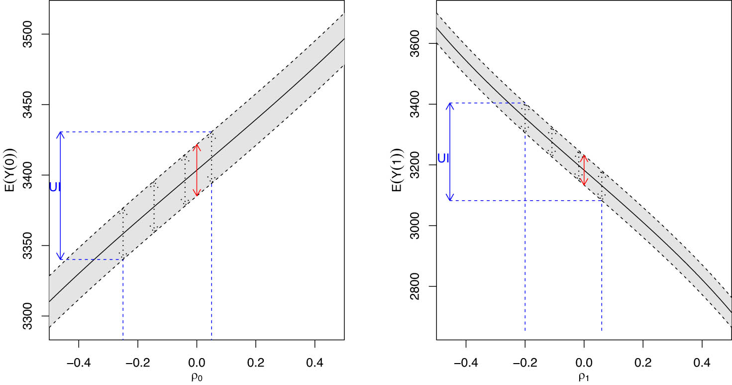
Estimates of average birth weight under smoking and non-smoking during pregnancy are given in the right and left plots, respectively; using output from ui.causal function (hdim.ui package). Solid black lines for bias-corrected AIPW estimates, τ ˆ AIPW refit − b ˆ refit , and 95% confidence intervals (gray area). Red intervals are confidence intervals assuming no unobserved confounding ( ρ t = 0 , t = 0,1 ), and blue intervals are 95% uncertainty intervals (using − 0.25 ≤ ρ 0 ≤ 0.05 and − 0.20 ≤ ρ 1 ≤ 0.06 ).

The difference in conclusions may be due to the fact that Nabi et al. [24] analysis excludes the unconfoundedness situation as one of the possible scenarios while ours do not. This discrepancy might be due to different modeling assumptions and thereby different influence functions and corresponding estimation procedures. For instance, Nabi et al. [24] sensitivity model establishes a link between the observed and unobserved potential outcome densities, which necessitates the requirement of common supports; a condition stating that the support of each of the missing potential outcomes must be a subset of the support of the corresponding observed potential outcome. This assumption may affect the validity of the results (see Section 7 in [16]). Furthermore, our method only uses clinical assumptions for bounding sensitivity parameters, whereas Nabi et al. [24] uses those assumptions for both selecting a valid tilting function (defining the sensitivity model) and bounding sensitivity parameters. The effect on their analysis of using alternative tilting functions is unclear to us.

5 Discussion

Unobserved confounding cannot be discarded nor empirically investigated in observational studies, and therefore, sensitivity analysis to the unconfoundedness assumption should be common practice. Moreover, high-dimensional settings are typical in observational studies using large data sets and machine learning for nuisance models. We have presented here a novel method to conduct sensitivity analysis in such situations using uniformly valid estimators, which is essential in high-dimensional setting. In particular, the sensitivity analysis proposed is based on the construction of an uncertainty interval for the causal effect of interest which we show has uniformly valid coverage. Finite sample experiments confirm the asymptotic results.

We use a sensitivity model with a sensitivity parameter, a correlation, which is easy to interpret and discuss with subject-matter scientists [23]. As all sensitivity models, ours describes potential departures from the unconfoundedness assumption. If sensitivity is detected as is the case in the presented application on the effect of smoking on birth weight, then this is important information. If no sensitivity is detected, then one might argue that this does not preclude the analysis to be sensitive to other departures from the unconfoundedness assumption. Note that our results show that we need to let ρ tend to zero with increasing sample size unless we can estimate bias due to unobserved confounding, and hence the propensity score, with a root-n convergence rate. An alternative to bias estimation is to fix the bias itself as the sensitivity parameter, at the expense of interpretability. Finally, future directions for research include generalizing our results from binary to continuous treatments, from continuous to binary outcome, as well as considering ultra-high dimensional situations ( p ≫ n ), which have their own challenges [39].

6 Supplementary material

Supplementary material contains additional simulation results and is available online.

References

[1] Fisher R. Cigarettes, cancer, and statistics. Centen Rev Arts Sci. 1958;2:151–66. Search in Google Scholar
[2] Rubin DB. Estimating causal effects of treatments in randomized and nonrandomized studies. J Educat Psychol. 1974;66(5):688–701. 10.1037/h0037350Search in Google Scholar
[3] Rubin DB. Formal mode of statistical inference for causal effects. J Stat Plan Inference. 1990;25(3):279–92. 10.1016/0378-3758(90)90077-8Search in Google Scholar
[4] Cornfield J, Haenszel W, Hammond EC, Lilienfeld AM, Shimkin MB, Wynder EL. Smoking and lung cancer: Recent evidence and a discussion of some questions. J Nat Cancer Inst. 1959;22(1):173–203. Search in Google Scholar
[5] Robins JM, Rotnitzky A, Zhao LP. Estimation of regression coefficients when some regressors are not always observed. J Amer Stat Assoc. 1994;89(427):846–66. 10.1080/01621459.1994.10476818Search in Google Scholar
[6] Van der Laan MJ. Targeted learning: causal inference for observational and experimental data. New York: Springer Science & Business Media; 2011. 10.1007/978-1-4419-9782-1Search in Google Scholar
[7] Farrell MH. Robust inference on average treatment effects with possibly more covariates than observations. J Econ. 2015;189(1):1–23. 10.1016/j.jeconom.2015.06.017Search in Google Scholar
[8] Van der Laan MJ, Gruber S. Collaborative double robust targeted maximum likelihood estimation. Int J Biostat. 2010;6(1):17. 10.2202/1557-4679.1181Search in Google Scholar PubMed PubMed Central
[9] Chernozhukov V, Chetverikov D, Demirer M, Duflo E, Hansen C, Newey W, et al. Double/debiased machine learning for treatment and structural parameters. Econ J. 2018;21(1):C1–68. 10.1111/ectj.12097Search in Google Scholar
[10] Belloni A, Chernozhukov V, Hansen C. Inference on treatment effects after selection among high-dimensional controls. Rev Econ Stud. 2014;81(2):608–50. 10.1093/restud/rdt044Search in Google Scholar
[11] Moosavi N, Häggström J, de Luna X. The costs and benefits of uniformly valid causal inference with high-dimensional nuisance parameters. Stat Sci. 2023;38(1):1–12. 10.1214/21-STS843Search in Google Scholar
[12] Vansteelandt S, Goetghebeur E, Kenward MG, Molenberghs G. Ignorance and uncertainty regions as inferential tools in a sensitivity analysis. Stat Sin. 2006;16(3):953–79. Search in Google Scholar
[13] Genbäck M, de Luna X. Causal inference accounting for unobserved confounding after outcome regression and doubly robust estimation. Biometrics. 2019;75(2):506–15. 10.1111/biom.13001Search in Google Scholar PubMed
[14] Rosenbaum PR. Sensitivity analysis for certain permutation inferences in matched observational studies. Biometrika. 1987;74(1):13–26. 10.1093/biomet/74.1.13Search in Google Scholar
[15] Ding P, VanderWeele TJ. Sensitivity analysis without assumptions. Epidemiology (Cambridge, Mass). 2016;27(3):368–77. 10.1097/EDE.0000000000000457Search in Google Scholar PubMed PubMed Central
[16] Franks A, D’Amour A, Feller A. Flexible sensitivity analysis for observational studies without observable implications. J Am Stat Assoc. 2020;115(532):1730–46. 10.1080/01621459.2019.1604369Search in Google Scholar
[17] Bonvini M, Kennedy EH. Sensitivity analysis via the proportion of unmeasured confounding. J Amer Stat Assoc. 2022;117(539):1540–50. 10.1080/01621459.2020.1864382Search in Google Scholar
[18] Zhang B, Tchetgen Tchetgen EJ. A semi-parametric approach to model-based sensitivity analysis in observational studies. J R Stat Soc Ser A. 2022;185(S2):668–91. 10.1111/rssa.12946Search in Google Scholar PubMed PubMed Central
[19] Zhao Q, Small DS, Bhattacharya BB. Sensitivity analysis for inverse probability weighting estimators via the percentile bootstrap. J R Stat Soc Ser B. 2019;81(4):735–61. 10.1111/rssb.12327Search in Google Scholar
[20] Gabriel EE, Sjölander A, Sachs MC. Nonparametric bounds for causal effects in imperfect randomized experiments. J Amer Stat Assoc. 2023;118(541):684–92. 10.1080/01621459.2021.1950734Search in Google Scholar
[21] Copas JB, Li HG. Inference for non-random samples. J R Stat Soc Ser B (Stat Methodol). 1997;59(1):55–95. 10.1111/1467-9868.00055Search in Google Scholar
[22] Imai K, Keele L, Tingley D. A general approach to causal mediation analysis. Psychol Methods. 2010;15(4):309–34. 10.1037/a0020761Search in Google Scholar PubMed
[23] Cinelli C, Hazlett C. Making sense of sensitivity: extending omitted variable bias. J R Stat Soc Ser B Stat Methodol. 2019 12;82(1):39–67. 10.1111/rssb.12348Search in Google Scholar
[24] Nabi R, Bonvini M, Kennedy EH, Huang MY, Smid M, Scharfstein DO. Semiparametric sensitivity analysis: unmeasured confounding in observational studies. Biometrics. 2024;80(4):ujae106. 10.1093/biomtc/ujae106Search in Google Scholar PubMed
[25] Scharfstein D, Rotnitzky A, Robins J. Rejoinder to comments on “adjusting for non-ignorable drop-out using semiparametric non-response models?”. J Amer Stat Assoc. 1999;94:1121–46. 10.2307/2669930Search in Google Scholar
[26] Farrell MH. Robust inference on average treatment effects with possibly more covariates than observations. 2018. arXiv:13094686v3. Search in Google Scholar
[27] Kennedy EH. Semiparametric theory and empirical processes in causal inference. In: He H, Wu P, Chen D-G, editors. Statistical causal inferences and their applications in public health research. Cham: Springer; 2016. p. 141–67. 10.1007/978-3-319-41259-7_8Search in Google Scholar
[28] Ghasempour M, Moosavi N, de Luna X. Convolutional neural networks for valid and efficient causal inference. J Comput Graph Stat. 2024;33(2):714–23. 10.1080/10618600.2023.2257247Search in Google Scholar
[29] Luedtke AR, Diaz I, van der Laan MJ. The statistics of sensitivity analyses. UC Berkeley Division of Biostatistics Working Paper Series Working Paper 341. 2015. Search in Google Scholar
[30] Gustafson P, McCandless LC. When is a sensitivity parameter exactly that? Stat Sci. 2018;33(1):86–95. 10.1214/17-STS632Search in Google Scholar
[31] Hines O, Dukes O, Diaz-Ordaz K, Vansteelandt S. Demystifying statistical learning based on efficient influence functions. Am Stat. 2022;76(3):292–304. 10.1080/00031305.2021.2021984Search in Google Scholar
[32] Gorbach T, de Luna X. Inference for partial correlation when data are missing not at random. Stat Probab Lett. 2018;141:82–9. 10.1016/j.spl.2018.05.027Search in Google Scholar
[33] Tibshirani R. Regression shrinkage and selection via the lasso. J R Stat Soc Ser B (Methodological). 1996;58(1):267–88. 10.1111/j.2517-6161.1996.tb02080.xSearch in Google Scholar
[34] R Core Team. R: A language and environment for statistical computing. Vienna, Austria; 2019. Available from: https://www.R-project.org/. Search in Google Scholar
[35] Chernozhukov V, Hansen C, Spindler M. hdm: high-dimensional metrics. R J. 2016;8(2):185–99. 10.32614/RJ-2016-040Search in Google Scholar
[36] Friedman J, Hastie T, Tibshirani R. Regularization paths for generalized linear models via coordinate descent. J Stat Soft. 2010;33(1):1–22. 10.18637/jss.v033.i01Search in Google Scholar
[37] Almond D, Chay KY, Lee DS. The costs of low birth weight. Q J Econ. 2005;120(3):1031–83. 10.1162/003355305774268228Search in Google Scholar
[38] Cattaneo MD. Efficient semiparametric estimation of multi-valued treatment effects under ignorability. J Econ. 2010;155(2):138–54. 10.1016/j.jeconom.2009.09.023Search in Google Scholar
[39] Tang D, Kong D, Pan W, Wang L. Ultra-high dimensional variable selection for doubly robust causal inference. Biometrics. 2023;79(2):903–14. 10.1111/biom.13625Search in Google Scholar PubMed
[40] Bishop YM, Fienberg SE, Holland PW. Discrete multivariate analysis: theory and practice. New York: Springer Science & Business Media; 2007. Search in Google Scholar
© 2025 the author(s), published by De Gruyter
This work is licensed under the Creative Commons Attribution 4.0 International License.
Articles in the same Issue
- Research Articles
- Decision making, symmetry and structure: Justifying causal interventions
- Targeted maximum likelihood based estimation for longitudinal mediation analysis
- Optimal precision of coarse structural nested mean models to estimate the effect of initiating ART in early and acute HIV infection
- Targeting mediating mechanisms of social disparities with an interventional effects framework, applied to the gender pay gap in Western Germany
- Role of placebo samples in observational studies
- Combining observational and experimental data for causal inference considering data privacy
- Recovery and inference of causal effects with sequential adjustment for confounding and attrition
- Conservative inference for counterfactuals
- Treatment effect estimation with observational network data using machine learning
- Causal structure learning in directed, possibly cyclic, graphical models
- Mediated probabilities of causation
- Beyond conditional averages: Estimating the individual causal effect distribution
- Matching estimators of causal effects in clustered observational studies
- Ancestor regression in structural vector autoregressive models
- Single proxy synthetic control
- Bounds on the fixed effects estimand in the presence of heterogeneous assignment propensities
- Minimax rates and adaptivity in combining experimental and observational data
- Highly adaptive Lasso for estimation of heterogeneous treatment effects and treatment recommendation
- A clarification on the links between potential outcomes and do-interventions