Decision making, symmetry and structure: Justifying causal interventions
-
David O. Johnston
 ,
Cheng Soon Ong
,
Cheng Soon Ong

Abstract
We can use structural causal models (SCMs) to help us evaluate the consequences of actions given data. SCMs identify actions with structural interventions. A careful decision maker may wonder whether this identification is justified. We seek such a justification. We begin with decision models, which map actions to distributions over outcomes but avoid additional causal assumptions. We then examine assumptions that could justify causal interventions, with a focus on symmetry. First, we introduce conditionally independent and identical responses (CIIR), a generalisation of the IID assumption to decision models. CIIR justifies identifying actions with interventions, but is often an implausible assumption. We consider an alternative: precedent is the assumption that “what I can do has been done before, and its consequences observed,” and is generally more plausible than CIIR. We show that precedent together with independence of causal mechanisms (ICM) and an observed conditional independence can justify identifying actions with causal interventions. ICM has been proposed as an alternative foundation for causal modelling, but this work suggests that it may in fact justify the interventional interpretation of causal models.
1 Introduction
Sometimes we want to make decisions supported by data. Structural causal models (SCMs) are a standard framework for addressing this kind of problem. In these models, variables of interest are identified with the nodes of a directed graph, and directed edges represent causal relationships between them. A decision maker using an SCM could bring any amount of prior information to the problem: at one extreme, the graph may just be a convenient means of representing facts about the consequences of actions that they already know to be true. At the other, a decision maker could have very little idea which graph is appropriate for their problem and may want to engage in causal discovery, where they employ general principles along with the given data to decide on a set of viable causal graphs.
Well-known difficulties of causal inference are that there are no widely accepted principles of causal discovery that will always yield a unique causal graph, and available data are typically consistent with causal graphs that admit a wide variety of interventional consequences. Even if these problems could somehow be avoided and a graph with nontrivial causal implications obtained, a decision maker must also decide how to map their available options to structural interventions on this graph. However, if the construction of the appropriate causal graph is beyond the decision maker’s prior knowledge, then the identification of options with structural interventions may also lie beyond their knowledge.
Consider, for example, an author who wants to know what genre to pick for their next writing project in order to maximise sales – science fiction or romance. Suppose they have collected a large dataset, and according to some causal discovery method, they have obtained a structural causal model (1)[1]. This model contains three variables: sales in the book’s first 12 months of life

Under the operation of a perfect intervention, given a distribution
The author can observe their own average sales
However, the event
It would be convenient if interventions on an SCM informed us about the consequences of ordinary attempts to manipulate the intervened variable. Convenience is not, in and of itself, a good reason to believe it is true. What we actually want is a sound reason to believe it:
It follows from plausible assumptions that ordinary attempts to manipulate are well modelled by interventions on an SCM derived from causal discovery.
It is empirically observed that SCMs derived from causal discovery accurately predict the consequences of ordinary attempts to manipulate the intervened variable.
One view is that decision problems with multiple means to manipulate a variable are ill-posed. Ambiguous interventions refer to the case where an intervention targets a variable that is a composite of a set of finer grained variables (in the same way, the genre of a book is a composite of the book’s textual contents, appearance, the cultural context in which it is interpreted and so forth). The previous work by Spirtes and Scheines has argued that composite variables do not have clear intervention semantics [6]. Pearl appears to have advanced a similar view: “there is no way a model can predict the effect of an action unless one specifies which variables are affected by the action and how.” [7, Ch. 11]
This is a strict principle which seems to rule out common patterns of causal reasoning. Is it really necessary to model each possible strategy in great detail to conclude that the nature of health benefits for many weight control strategies are likely to be similar, given similar success at controlling one’s weight? What’s more, just how much detail does one need to specify about which variables are affected? We cannot possibly specify everything about which variables a given action affects. Adopting a different diet will lead one to walk down different aisles at the supermarket, use different cookware to prepare food and imbue their kitchen with different scents – but one need not manually rule out the relevance of these and every other possible impact of shifting diet to conclude that an overweight person who adopts a high protein diet and loses weight will also reduce their risk of heart disease.
Reviewing the general issue, it is clear that SCMs can be used to predict the consequences of actions in systems we already understand – it is easy to construct toy models of familiar systems like sprinklers, rain and footpaths where the results of intervention operations match the already known consequences of actions. It is less clear how to apply them to predict the consequences of actions in systems that are less understood. On one hand, it may be possible to learn SCMs from data according to general principles of causation. On the other hand, a decision maker has a set of pragmatic actions they are considering which must be mapped to interventions in the learned SCM. It is difficult to find a method for doing this mapping that is both valid and avoids throwing away a lot of the utility of causal modelling.
We don’t know how to resolve the problem as posed, so we take a different approach. We only aim to help a decision maker predict the consequences of their pragmatic actions, and to offer general principles they can use to improve their predictions with data. Intervention operations, as defined on SCMs, have no role in this process unless they are justified by the learning principles and the data. What we show, in the end, is that sometimes they are justified.
Decision models are a formal representation of models that help a decision maker predict the consequences of their actions. They map a set of actions, assumed to be known to the decision maker, to probability distributions representing predictions of consequences. Such models have been studied previously by numerous authors [8–12]. To be useful, a decision model must come with some means of relating observed data to consequences of actions. Interventions on structural models are one such means – an intervention on a variable
The first principle we consider is a generalisation of the assumption of independent and identically distributed (IID) variables. Specifically, we consider decision models with sequences of variable pairs that share independent and identical responses (IIR), where the distribution of every “output” variable conditional on the corresponding “input” variable is identical, regardless of whether it represents previously observed data or future data that will be affected by the actions of the decision maker, no matter what action is taken. Much like structural interventions, this assumption holds that the identified conditional distributions are not changed by the actions of the decision maker.
To help us think about when the IIR assumption might be justified, we relate it to a symmetry of decision models inspired by De Finetti’s representation theorem [13]. We prove that an IIR decision model with an unknown response function is equivalent to an input–output contractible (IO-contractible) decision model (Theorem 3.17). As far as justifying the IIR assumption, this is a negative result. IO-contractibility implies the interchangeability of sufficiently large quantities of previously observed data with any data arising from experimentation – a condition which is usually unreasonable. This is analogous to the common view that causal effects are typically not known to be identified in observational data.
An alternative learning principle is that of precedent. This is the assumption that – informally stated – all of the decision maker’s prospective actions have been taken before under all of their possible circumstances, and their consequences are observed in the available data. This differs from the IIR assumption in that the decision maker does not know which observations go with a particular action and particular set of circumstances. It is analogous to starting with an IIR sequence and forgetting the inputs. Because consequences will generally have a different distribution of inputs, forgetting the inputs means the observed data is no longer interchangeable with the consequences. Our key result (Theorem 4.7) combines precedent with an additional assumption: absolute continuity of conditionals (ACC). These two assumptions – precedent and ACC – together with an observation of conditional independence imply IIR holds with respect to a pair of observed variables, and so they justify treating our actions as interventions on the input variable identified by the theorem.
ACC is not a simple assumption to state: it requires that certain “higher order” probability distributions over conditional distributions remain absolutely continuous with respect to the Lebesgue measure after observing a conditional independence. We can gain an intuitive understanding of this assumption by relating it to the principle of independent causal mechanisms [14], an informal principle that says “causal mechanisms” – which are conditional distributions of effects given their parents – are in some sense independent or at least are not deterministically dependent on one another. We show that, given a particular version of the principle of independent causal mechanisms, the assumption of absolute continuity of conditionals can be justified by assuming the direction of causal relationships between certain variables. Thus, given a decision model, we offer a justification for treating actions as interventions on certain variables based on precedent (a kind of symmetry) ACC (justified by causal structure) and an observed conditional independence.
Structural causal models are usually taken to uphold the principle of independent causal mechanisms and to support the assumption that the consequences of choices can be computed via intervention operations [15]. However, logically speaking, these are separate assumptions. Our result suggests that, if we already accept the principle of independent causal mechanisms, we may be able to reduce the assumption of interventions to a symmetry (precedent) and an observed feature of the world (conditional independence).
1.1 Connections to previous work in causal inference
Our starting point is that we want models that are useful for decision makers, which motivates the formalism of “decision models.” This approach is in the tradition of the decision theoretic approach to causal inference that has been applied in slightly different ways by previous works [8–10]. Probabilistic graphical models [11], while not explicitly decision theoretic, have much in common with the decision models we study. They are sufficiently similar that methods for computing the consequences of interventions in probabilistic graphical models [12] can be adapted to decision models.
Another precursor to our work is the notion of a sequence of exchangeable observations along with “one more (possibly non-exchangeable) observation” [16]. This anticipates our effort, with the CIIR assumption, to extend the assumption of exchangeability for previously observed data to an assumption that can also apply to future data subject to a decision maker’s influence. While Lindley mentioned that this approach can be applied questions of causation, he did not explore this deeply due to the perceived difficulty of finding a satisfactory definition of causation.
There have been a number of other works on symmetries in causal inference. Models with exchangeable potential outcomes have been used to prove several identification results [17,18]. There are similarities between exchangeable potential outcomes and independent and identical response functions. Given our focus on the relationship between our approach and the structural approach to causal modelling, a thorough treatment of similarities and differences between our approach and the potential outcome approach is beyond the scope of this article.
Conditional exchangeability is defined as the exchangeability of the non-intervened causal parents of a target variable under intervention on its remaining parents [19]. Sareela et al. suggested that this could be interpreted as a symmetry of some kinds of experiment: if, for example, patients are administered a treatment, then conditional exchangeability can be viewed as an expected invariance of results when patients in the experiment (and their concomitant treatments) are exchanged. Similar kinds of symmetry appear in several other works [10,20–23]. A key difference between all of these causal symmetries and input–output contractibility is that these are all symmetries that involve altering an experiment. Input–output contractibility, which we study, is symmetry with respect to data manipulation – under IO contractibility, certain permutations and subsets of the data have exactly the same model. Thus, IO contractibility can be defined entirely using the mathematics of decision models, without having to discuss potentially complex manipulations of hypothetical experiments.
A different kind of regularity of causal models is given by the stable unit treatment distribution assumption (SUTDA) [10] and the stable unit treatment value assumption (SUTVA) [17]. This regularity is similar to the condition of locality, a subassumption of input–output contractibility, and as with exchangeable potential outcomes, a careful examination of the similarities and differences is beyond the scope of this article.
Theorem 4.7 was inspired by causal inference by invariant prediction [24]. While both the assumptions and the conclusions drawn in that work differ from the assumptions and conclusion of Theorem 4.7, both look for variable pairs
An alternative which exchangeability-like symmetry can be used to learn causal structure [25], in contrast to our work where we use structure together with symmetry for the purposes of predicting consequences of actions from data, but do not consider the problem of learning structure from data.
1.2 Outline
Section 2 outlines our mathematical framework and provides a brief reference on notation. Section 3.2 introduces decision models with conditionally independent and identical responses, a generalisation of conditionally independent and identically distributed variables. We then introduce and explain Theorem 3.17, a generalisation of De Finetti’s representation theorem that applies to decision models, and argue on the basis of this theorem that the assumption of conditionally independent and identical responses is often unreasonable.
Section 4 introduces the notion of precedent and then proves Theorem 4.7, which establishes that precedent, together with ACC and an observed conditional independence implies conditionally independent and identical responses for pairs of observed variables. We also show how ACC can be justified by structural assumptions, if we accept the principle of independent causal mechanisms.
2 Technical prerequisites
This section gathers some necessary technical definitions, and is included for reference. A reader who wishes to follow the arguments of the article may skip to Section 3 and refer back to this section as required.
Section 2.1 introduces the notation used in this article. Because decision models are stochastic functions rather than probability measures, we introduce in Section 2.2 some extensions of standard probabilistic concepts.
2.1 Notation
We refer readers to chapters 1, 2 and 4 of [26] for an introduction to probability theory as we use it. Here, we offer a brief overview of our notation.
We denote a measurable space
We write random variables
A sequence of random variables
We denote by
We use the Iverson bracket
A positive integer in square brackets
The set
2.2 Decision models
We are interested in modelling decision making rather than prediction. A decision maker makes a choice of one of a set of different options, and different choices lead to different outcomes. This is not the case for someone only interested in prediction, as the outcome is unaffected by the prediction “chosen.”
Choices differ from ordinary random variables. When we begin thinking about a decision problem, we do not know which choice we will make (or else the problem would be trivial). When we finish thinking about it, the choice has been made. Random variables are not like this – we are uncertain about them at the outset, and we remain uncertain when we have constructed a satisfactory probabilistic model. There may be many interesting things to say about the process of making a decision, but we will not say them here. The decision maker has a set of options or choices that they may choose, and we do no speculation about which choice will be made; there is no probability distribution associated with the set of options (for further argument that option probabilities should not contribute to decision making [27]).
A decision maker does require, for each of their options, a forecast of the consequences. We model this with a Markov kernel, a function that maps options to probability distributions.
Definition 2.1
(Markov kernel) Given measurable spaces
The map
The map
We use an alternative notation for the signature of a Markov kernel to stress the fact that we can consider it a measurable map from a measurable set to a set of probability distributions.
Notation 2.2
(Signature of a Markov kernel) Given measurable spaces
A decision model is a generalisation of a probability space. A probability space is a measurable sample space together with a probability measure. A decision model is a measurable option set, a measurable sample space and a Markov kernel that maps options to probability measures on the sample space. We represent the Markov kernel as
Definition 2.3
(Decision model) A decision model is a triple
Random variables are measurable functions on the sample space.
Definition 2.4
(Random variable) Given a decision model
We use
2.3 Conditional distributions and conditional independence in decision models
Decision models yield a probability distribution for each option
We use two notions of conditional independence. The first is conditional independence for each option
The second notion is independence “of
Extended conditional independence is a generalisation that subsumes both of these versions of conditional independence [28].
Our notion of conditional independence satisfies the standard properties as long as we insist that
Symmetry:
Decomposition:
Weak union:
Contraction:
If
In a decision model, we say that two random variables are almost surely equal if they are almost surely equal for every
We also have a notion of almost sure equality for conditional distributions. Given two conditional distributions
2.4 Directed graphs
We refer to structural causal models in several places. The theory of structural models that we use can all be found in Chapter 1 of [7]. We use the notion of an intervention and d-separation (which we represent with the
3 Inferring consequences when observations and consequences share identical responses
Recall the example discussed in Section 1: an author wants to choose the genre of a book they will write. There, we proposed a structural causal model that predicted that the distribution of sales conditional on genre, the author’s historical sales success and global trends sales does not change under intervention on genre. We also raised the question of how the author could know, exactly, if the action they took was an intervention – or close enough to it – to take advantage of this invariance.
Consider a slightly different notion of invariance: instead of assuming the distribution of sales conditional on genre and the covariates not change under an intervention on genre, assume it doesn’t change under any of the author’s available actions. In this case, the author can reason as follows: while they don’t know exactly what consequences deciding to write a romance novel (
If the author accepts the second assumption (and we’re not saying that they should), then they can treat all of their actions that control the genre of their book as interventions on genre with respect to the original causal model (not necessarily perfect interventions). We are not suggesting the author should accept this assumption, just that if they did, then they could model their actions as interventions. The work in this article serves as a foundation for the more plausible justification we present in the Section 4.
In the language of decision models: the author has a decision model
We call
Thus, the notion of a “fixed response function” has two sub-assumptions: first, conditional on
Is it ever reasonable to assume CIIR? It might be for systems deliberately engineered for regularity. A switch reliably turns on a light if you flick it, and a function in a piece of code reliably returns the same result given the same input. Book sales or human health are not examples of systems like this, however. Maybe in principle many non-engineered systems exhibit regular responses, but we generally don’t know if any particular collection of variables will do so.
Instead of appealing to our prior knowledge of mechanisms as we do in the case of engineered systems, we could try to appeal to knowledge of symmetries of the problem. The inspiration for this approach comes from De Finetti’s work on Bayesian probabilistic inference. De Finetti observed that many statistical models assumed a sequence of independent and identically distributed random variables conditional on an unknown “true parameter” (which we could call conditionally independent and identically distributed or CIID). He was unsatisfied with the notion of “true parameters” and offered an alternative way to analyse these models via symmetry. If a prediction problem is not changed in any important way by permuting the measurements, then it seems reasonable to adopt a probability model that is unchanged under permutation of variables. De Finetti showed that the class of probability models with this symmetry (called exchangeability) is equivalent to the class of CIID models [13].
Here, we ask: is there an analogous indifference over permutations in decision models that yields the CIIR assumption? Formally, the answer is yes: the class of CIIR decision models is equivalent to decision models with a symmetry we call input–output contractibility (or IO contractibility). However, IO contractibility is a less intuitive and less appealing assumption than exchangeability. The main practical upshot of this section is an argument against assuming CIIR in many situations. IO contractibility implies that, after having seen infinite data, any further input–output pairs can be exchanged. Setting aside the infinite data requirement, if the author assumes CIIR for a decision model that includes both a convenient historical dataset of book sales and for the sales of their own books, they accept that these two problems are identical:
Write a large number of books of various genres themselves, observe their sales, and predict the sales of one more book they write of a given genre.
Observe the sales, genres and author averages of the same number of books from the convenient historical dataset, and use this to predict the sales of one book they write of a given genre.
IO contractibility implies that, after having seen infinite data, any further input–output pairs can be exchanged. Setting aside the infinite data requirement, if the author assumes CIIR for a decision model that includes both a convenient historical dataset of book sales and the sales of their own books, they accept that these two scenarios are equivalent for predicting the author’s future book sales:
Writing a large number of books of various genres themselves and observing their sales
Observing the sales and genres of a large number of books from the convenient historical dataset
However, there are good reasons to think that the past sales of the author’s own books, written under similar conditions, will be much more informative about their future book sales than the sales of books by an arbitrary collection of third parties under unknown conditions. While it’s possible that the historical dataset could be as predictive as the author’s own experience, assuming this equivalence from the outset is not justified.
3.1 Conditionally independent and identical responses
We now turn to the formal treatment of the CIIR assumption and its equivalence to IO contractibility. First, we define sequential input–output models as a shorthand for decision models that feature a sequence of random variable pairs.
Definition 3.1
(Sequential input–output model) A decision model
In general, the relationship between the decision maker’s choice and the behaviour of inputs
Sequential input–output pairs
Definition 3.2
(Conditionally independent and identical responses) Given a sequential input–output model
This is a general form of the CIIR assumption that only requires the outputs
Definition 3.3
(Weakly data-independent) A sequential input–output model
3.2 Symmetries of sequential conditional probabilities
Given the previously mentioned sequences
We wish to express the assumption that, setting aside the fact that we learn more about these pairs as we observe more data, as far as the decision maker is concerned they are equivalent in terms of behaviour. Following the example of exchangeability, one possible way to express this is that swapping pairs makes no difference to the model – under this assumption,
This assumption is stronger than necessary. Even if the
Example 3.4
Suppose there is a machine with two arms
because
because
From the point of view of the DM, the good arm always turns out to be the one that the first person picks, no matter what they pick – and only the arm the first person picks. The first and second person’s choices are not interchangeable.
This model only requires that the first person’s choice resolve the decision maker’s uncertainty about the payout function
Example 3.4 motivates the weaker symmetry we call exchange commutativity. The key difference is that exchange commutativity allows for the permutation of pairs after conditioning on some variable
Definition 3.5
(Exchange commutativity) Given a sequential input–output model
We require an additional regularity assumption, which we call locality. We’re going to state the assumption first, then give an example (involving inflation) to illustrate why this assumption is needed. Intuitively, locality says something like “
As Example 3.4 suggests, locality cannot be the assumption that
Definition 3.6
(Locality) Given a sequential input–output model
If an input–output model is both exchange commutative and local with respect to the same
Definition 3.7
(Input–output contractibility) A sequential input–output model
Theorem 3.8
(Equality of equally sized conditionals) Given a sequential input–output model
Proof
Appendix B.1.□
Appendix B.2 explores out two additional properties of these two symmetries. Example B.5 shows that neither locality nor exchange commutativity is implied by the other. Example B.6 shows that locality by itself does not rule out everything that we might intuitively describe as “interference” between pairs.
We might wonder if both locality and exchange commutativity are needed, seeing as exchange commutativity by itself looks like a generalisation of exchangeability – in fact, if we take the inputs to be trivial, then it coincides precisely with exchangeability. The reason why locality is also needed is that, for nontrivial inputs, we can construct exchangeable commutative models where the response function depends on a symmetric function of the full set of inputs
3.3 Representation of IO contractible models
In this section, we state Theorem 3.17: a sequential input output model
The proof of the theorem can be found in its entirety Appendix B.3. There we employ a string diagram notation in some steps of the proof, itself explained in Appendix A. Here, we introduce enough to explain the the theorem statement.
3.4 Preliminaries
Definition 3.9
(Input count variable) Given a sequential input–output model
That is,
If we have an infinite sequence of pairs
Definition 3.10
(Tabulated conditional distribution) Given a sequential input–output model
That is, the
The directing random measure of an infinite sequence of exchangeable variables
Definition 3.11
(Directing random measure) Given a decision model
where each
Given input and output sequences
Definition 3.12
(Directing random conditional) Given a sequential input–output model
A finite permutation within columns is a function that independently permutes a finite number of elements in each column of a table. A special case of such a function is a permutation of rows that swaps entire rows; this is a permutation within columns that applies the same permutation to each column.
Definition 3.13
(Permutation within rows) Given a sequence of indices
Lemma 3.15 shows that an IO contractible conditional distribution can be represented as the product of a probability distribution symmetric to permutations of rows and a “lookup function” or “switch.” Lookup function is also used in the representation of potential outcomes models [17], but we do not assume that the tabulated conditional
To prove Lemma 3.15, we assume that the set of input sequences in which each possible value appears infinitely often has measure 1 for every option in
Definition 3.14
(Almost surely infinite) Given a sequential input–output model
we have
Note that for any
The key property of the tabulated conditional is that we can evaluate the regular conditional
Lemma 3.15
Suppose a sequential input–output model
and for any finite permutation within columns
Proof
Sketch only.
Only if: We define a random invertible function
If: We construct a conditional probability satisfying equations (2) and (3) and verify that it satisfies IO contractibility.
The full proof can be found in Appendix B.3. Note that the proof uses string diagram notation explained in Appendix A.□
Because the distribution
Theorem 3.16
Suppose a sequential input–output model
Proof
The strategy we pursue is to show that an arbitrary subsequence of
The proof is in Appendix B.3.□
3.5 Statement of the representation theorem
We are now ready to state the main result of this section, Theorem 3.17. Assuming a weakly data independent model
Theorem 3.17
(Representation of IO contractible models) Suppose a weakly data-independent sequential input–output model
There is some
For all
There is some
Proof
(1)
(3)
(2)
See Appendix B.4 for the full proof. Note that the proof uses string diagram notation explained in Appendix A.□
The presence of the
Theorem 3.18
A data-independent sequential input–output model
If in addition each
Proof
See Appendix B.5.□
3.6 Does IO contractibility help us infer consequences?
One of the key contributions of De Finetti’s representation theorem was to provide an alternative justification for the common modelling assumption that a sequence of variables were all distributed according to a shared but unknown “true distribution.” De Finetti regarded the notion of an “unknown true distribution” as nonsensical, and through his representation theorem suggested that we could instead justify this structure by arguing that the experiment that produced the sequence of variables was, from the point of view of the analyst seeking to make predictions, invariant to reindexing the variables in the sequence.
Can IO contractibility help to justify common causal assumptions in a similar way? The answer generally seems negative: Theorem 3.18 tells us IO contractibility implies regarding “experimental” and “observational” data as interchangeable provided we have enough of each, but we normally wouldn’t consider datasets collected under meaningfully different conditions to be interchangeable.
Suppose our author has written 1,000 books of their own, and let
This is the basis for our claim at the start of this section that, under the CIIR assumption, the author is obliged to ignore any data related to the consequences of their own actions if they are given enough passive observations to start with. If we loosely associate “consequences of observations” with experimental data, we can note that in practice, when both experimental and observational data are available, they are not assumed to be interchangeable in this sense – in fact, the question of how well the observational data predicts experimental outputs is one of substantial interest [30–32].
To cut a long story short, CIIR is not a compelling assumption for inferring consequences from data. The question arises: what else can we do?
4 Inferring consequences when choices have precedent
Given a convenient dataset of passive observations and a desire to predict the consequences of one’s actions, it is generally unreasonable to treat (sufficiently large) sequences of passive observations as interchangeable with sequences of direct observations of the consequences of actions. A decision maker ought to give some weight to the possibility that in the long run these sequences exhibit different patterns and, equivalently, they should not accept the CIIR assumption. How can a decision maker express the idea that the consequences of their actions are in some sense like previous observations of a similar system, without making an overly strong assumption like CIIR? A common move is to invoke unobserved variables: assume that there is a consistent input–output relationship provided all of the inputs are observed, but it is not known what all of the inputs are. We make the same assumption here.
By itself, this assumption can be trivial. If we have inputs
We explore an alternative constraint: the distribution of
In order to derive a useful inference rule, we require another assumption we call absolute continuity of conditionals. As a technical assumption it is quite opaque, but we can gain some intuition for it via the informal principle of independent causal mechanisms. We save the details for Section 4.2, but briefly: assuming a particular form of the principle of independent causal mechanisms, the assumption of absolute continuity of conditionals can be justified by assumptions about the directions of causal relationships between certain variables. Precedent and absolute continuity of conditionals together yield Theorem 4.7, which allows us to infer that observed pairs of variables exhibit conditionally independent and identical responses from conditional independence.
The following example illustrates the general idea we discuss here.
Example 4.1
Suppose a decision maker collects data about a group of people who have variously engaged the services of dieticians, sporting coaches, general practitioners, bariatric surgeons and none of the above, with practitioner choice recorded by the variable
Our decision maker presumes that each group of people
This inference might fail if, for any reason, treatment plan were selected in a way that masks the variation in their effects. For example, if all groups of people overwhelmingly choose to pursue diet changes in the end, then their results will not reveal any variation in mortality outcomes due to different treatment strategies. Alternatively, it might be the case that unobserved variables are delicately balanced just so that the conditional independence holds. For example, perhaps holding final BMI equal diet interventions tend to produce better health than bariatric surgery, but the visitors to the surgeon are exactly enough healthier than visitors to dieticians to make the final outcomes for both groups identical.
4.1 Passive data, consequences, and precedent
To simplify the presentation, we will consider a specific kind of decision model featuring a long sequence of passive observations indexed by natural numbers. Passive observations are completely unresponsive to the decision maker’s choice. This is augmented with one more random variable representing the consequences of acting, indexed by the special character
Definition 4.2
(Passive data and consequences) Given a decision model
We will also deal with models with the following standard structure:
Definition 4.3
(Latent CIIR model) A latent CIIR model is a model
We can take any model
Theorem 4.7 establishes sufficient conditions for the informal deduction described in Example 4.1. We assume that all variables of interest are discrete, and will make use of an alternative notation for discrete conditional probabilities.
Definition 4.4
(Index notation for discrete conditional distributions) Given a joint probability distribution
With regard to precedent, we specifically want to assume that the achievable distributions of inputs to
Definition 4.5
(Precedent) Given a latent CIIR model
We say that the consequences have
When we have precedent, we can compute the distribution of consequences
A further assumption for Theorem 4.7 is one we call absolute continuity of conditionals (ACC). The basic idea is that, after a decision maker decides that
Definition 4.6
(Absolute continuity of conditionals [ACC]) Given a latent CIIR model
We say that the options
where
Theorem 4.7 tells us: if we assume
Theorem 4.7
(Latent to observable IO contractibility) Given a latent CIIR model
Let
i.e.
If
Proof
We show that the assumption of conditional independence imposes a polynomial constraint on
Full proof is presented Appendix C.□
4.2 Justifying the assumptions of Theorem 4.7
4.2.1 Structural justifications for ACC
We’ve offered some motivation for the assumption of precedent, but not yet for the assumption of absolute continuity of conditionals. Justifying this assumption is not straightforward: while it’s common to assume parameters are unconditionally distributed absolutely continuously with respect to the Lebesgue measure, this assumption involves conditioning on the event
We can make a case for preferring this interpretation by appealing to assumptions typically used to justify causal discovery. Those assumptions are, informally:
In structural causal models, missing edges are common.
The causal mechanisms encoded by structural models are not precisely aligned.
The first assumption, more precisely, is that conditional independences may have positive probability if they correspond to a structural causal model with a missing edge. Such an assumption can be found in, for example, decomposable scoring rules [33], and it is present in spirit in causal discovery based on the faithfulness assumption.
The second assumption is derived from the informal notion that the “causal mechanisms” encoded by structural models are not precisely aligned – this is the principle of independent causal mechanisms [14][2]. There are multiple precise interpretations of this informal principle, and a version suitable for our purposes is given in [15]. Given a graph
A consequence of this is that if
Set this aside for a moment, and consider a causal discovery problem under the faithfulness assumption. Start with a particular set of hypothesised structural causal models: three observed variables,

Now, we observe that
This leaves us with the reduced set of structural models:

In every model in this collection,
We claim that
Recall that absolute continuity of conditionals is required to hold after accounting for the conditional independence. Thus, we consider the reduced set
Edge from
Edge from
No edge from
This identifies
4.2.2 Applying structural arguments for ACC
We have argued that a decision maker may infer that the conditional distribution of an output
The decision maker assumes the consequences of their actions have precedent in the observed data.
The decision maker supposes that the observed and unobserved variables supporting the precedent assumption have certain causal structures.
The decision maker observes a particular conditional independence.
There remain challenges to applying this theory to real-world decision problems. The first is shared with other theories of causal discovery from conditional independence: the result depends on the observation of exact conditional independence, but we can only ever observe approximate independence. This is a familiar problem for inferring causal relationships from conditional independence – see, for example, [34] where it is shown that spurious approximate conditional independences can be common in causal structures with sufficiently many edges.
To handle the case of approximate conditional independence, there are two assumptions we could explore strengthening in Theorem 4.7: precedent and absolute continuity of conditionals. Instead of precedent, we could consider bounds on the divergence between the distributions of
The second challenge is related to making assumptions about an unobserved variable

Under the standard interventional interpretation, the effect of
To illustrate with an example, suppose that our author observes in their historical data that book sales
Can we find a suitable
Instead of searching for a completely satisfactory theoretical justification for the required structural assumptions, we could empirically test the principle suggested by Theorem 4.7. We could, for example, test whether the optimist’s view generally holds up in practice, however compelling its theoretical motivation is. This would involve searching for datasets where there are variables
5 Conclusion
There seems to be a large gap between the set of things that people routinely learn to manipulate and the set of circumstances where contemporary theories of causal inference tell us that valid inference is possible. We would like to be able to close this gap; we want to be able to build systems that learn to manipulate the world at least as well as people do, and ideally we would like to understand how they learn to manipulate it. How to do this is a wide open question; there are many plausible approaches, and it is not yet clear which will be the most fruitful.
We explored the possibility that our understanding of causal inference is missing a fundamental principle – specifically, the principle of symmetry. Ordinary statistics gets a lot of mileage from the idea that no observation is “special”; one can be exchanged for another. To a decision maker, the consequences of their actions are always special, but they are not arbitrarily special. When I am facing a decision, I am usually aware that many other people have faced similar decisions, with access to similar information and similar capabilities and it would be foolish to think that the consequences of my actions are vastly different to consequences already observed. We proposed precedent as a symmetry principle that captures the idea that, while a decision maker may be somewhat special, they are not arbitrarily special, and we show how (in combination with the principle of independent causal mechanisms) this principle offers a novel justification for valid causal inference.
We believe this approach is promising for two main reasons. First, the assumption of precedent seems to us better motivated than the assumption that actions are modelled by causal interventions (though this is admittedly a judgement call). Second, standard structural models invoke two independent “structural” assumptions: interventions and the principle of independent causal mechanisms. Our framework, on the other hand, derives intervention-like inferences from the combination of precedent and the principle of independent causal mechanisms, suggesting that there may be a more parsimonious theory for interpreting causal structure. Much work remains to flesh out the theoretical foundations, elaborate applications and empirically test this approach, but we think it opens up promising and novel lines of research.
Acknowledgements
Thanks to members of the ANU College of Engineering and Computer Science for helpful discussion and feedback, especially Elliot Catt, Tom Everitt and Sarita Rosenstock.
-
Funding information: RW’s contribution was supported by the Deutsche Forschungsgemeinschaft under Germany’s Excellence Strategy – EXC number 2064/1 – Project number 390727645. DJ’s contribution was supported by an Australian Government Research Training Program Scholarship.
-
Author contributions: David O. Johnston conceived the project, developed the theoretical framework, wrote the proofs and drafted the manuscript. Robert C. Williamson and Cheng Soon Ong provided substantial guidance in developing and refining the theoretical ideas. All authors discussed the results and implications and commented on the manuscript.
-
Conflict of interest: No conflicts of interest to declare.
-
Data availability statement: Not applicable.
Appendix A String diagrams
We use a string diagram notation to represent probabilistic functions. This is a notation created for reasoning about abstract Markov categories and is somewhat different to existing graphical languages. The main difference is that in our notation wires represent variables and boxes (which are like nodes in directed acyclic graphs) represent probabilistic functions. Standard directed acyclic graphs annotate nodes with variable names and represent probabilistic functions implicitly. The advantage of explicitly representing probabilistic functions is that we can write equations involving graphics. This is introduced in Section A.
We make use of string diagram notation for probabilistic reasoning. Graphical models are often employed in causal reasoning, and string diagrams are a kind of graphical notation for representing Markov kernels. The notation comes from the study of Markov categories, which are abstract categories that represent models of the flow of information. For our purposes, we don’t use abstract Markov categories but instead focus on the concrete category of Markov kernels on standard measurable sets.
A coherence theorem exists for string diagrams and Markov categories. Applying planar deformation or any of the commutative comonoid axioms to a string diagram yields an equivalent string diagram. The coherence theorem establishes that any proof constructed using string diagrams in this manner corresponds to a proof in any Markov category [35]. More comprehensive introductions to Markov categories can be found in [36,37].
A.1 Elements of string diagrams
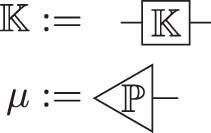
Markov kernels are drawn as boxes with input and output wires, and probability measures (which are Markov kernels with the domain
Given two Markov kernels

Given kernels

A space
Product spaces
A kernel

We read diagrams from left to right (this is somewhat different to [36–38] but in line with [35]), and any diagram describes a set of nested products and tensor products of Markov kernels. There are a collection of special Markov kernels for which we can replace the generic “box” of a Markov kernel with a diagrammatic elements that are visually suggestive of what these kernels accomplish.
A.2 Special maps
Definition A.1
(Identity map) The identity map
Definition A.2
(Erase map) Given some 1-element set

Definition A.3
(Swap map) The swap map

Definition A.4
(Copy map) The copy map

Definition A.5
(

A.2.1 Semidirect product
Given

The semidirect product is can be used to join a marginal
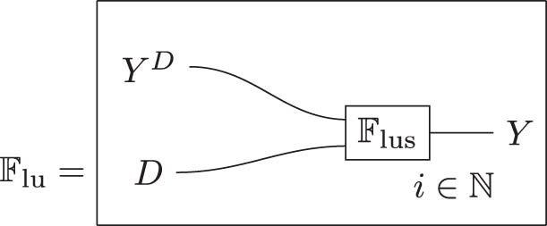
A.2.2 Plates
In a string diagram, a plate that is annotated
Thus, given

A.3 Commutative comonoid axioms
Diagrams in Markov categories satisfy the commutative comonoid axioms.


as well as compatibility with the monoidal structure

and the naturality of del, which means that

(we do not need a deeper understanding of naturality here)
A.3.1 Markov kernels associated with functions
For any measurable function
A.4 Manipulating string diagrams
A morphism in a Markov category is deterministic iff it commutes with the copy map.
Definition A.6
(Copy map commutes for deterministic morphisms) For
holds iff

Deterministic Markov kernels are the Markov kernels where, for any
Planar deformations along with applications of equations (A1) through equation (A4) give us a set of rules for transforming one string diagram into an equivalent one.
String diagrams can always be converted into definitions involving integrals and tensor products. A number of shortcuts can help to make the translations efficiently.
For arbitrary

That is, an identity map “passes its input directly to the next kernel.”
For arbitrary

That is, the copy map “passes along two copies of its input” to the next kernel in the product.
For arbitrary

The swap map before a kernel switches the input arguments.
For arbitrary

Given

Thus, the action of the
A.4.1 Labelling wires with variable names
The previous examples all labelled wires with spaces. Going forward, we will instead label wires with variable names. Given a decision model

The wire labels identify the diagram on the right as a picture of

The semidirect product of conditional distributions is the “joint conditional”:

B Symmetries of conditional probabilities
B.1 Equality of equally sized contractions
This is the proof of Theorem 3.8.
All swaps can be written as a product of transpositions, so proving that a property holds for all finite transpositions is enough to show it holds for all finite swaps. It’s useful to define a notation for transpositions.
Definition B.1
(Finite transposition) Given two equally sized sequences
that sends the
Lemma B.2 is used to extend conditional probabilities of finite sequences to infinite ones.
Lemma B.2
(Infinitely extended kernels) Given a collection of Markov kernels
then there is a unique Markov kernel
Proof
Take any
Furthermore, by the definition of the
Thus, by the Kolmogorov extension theorem [26], for each
Furthermore, for each
so by the Monotone convergence theorem, the sequence
Thus,
Corollary B.3
Given
for all
Proof
Fix arbitrary
Hence for all
and, in particular, by Lemma B.2,
Theorem B.4
Given a sequential input–output model
Proof
Only if: For a sequence of natural numbers
If
Use the fact that
if
then by Corollary B.3
Finally, by locality,
If: Taking
B.2 Examples of symmetries
These are the examples referenced in Section 3.2. Example B.5 shows that neither locality nor exchange commutativity is implied by the other.
Example B.5
We prove the claim by way of presenting counterexamples.
First, a model that exhibits exchange commutativity but not locality. Suppose
for some sequence
so
so
Next, a model that satisfies locality but does not commute with exchange. Suppose again
then
so
so
Although locality seems to an assumption that there is no interference between inputs and outputs of different indices, by itself, it actually permits models with certain kinds of interference. This is shown in Example B.6.
Example B.6
Consider an experiment where I first flip a coin and record the results of this flip as the outcome
Thus, the marginal distribution of both experiments in isolation is
B.3 Representation theorem preliminaries
This is the proof of Lemmas 3.15 and B.13 and Theorem 3.16 from Section 3.4. In addition, Lemmas B.13 and B.15 are presented and proved, which will be later used in the proof of Theorem 3.17.
Note that these proofs use the string diagram notation explained earlier in Appendix A. First, we will reproduce definitions of locality and exchange commutativity with equivalent statements in string diagram notation.
Definition B.7
Given a sequential input–output model

Definition B.8
Given a sequential input–output model
We say
The following definitions are also reproduced for the reader’s convenience.
Definition B.9
Given a sequential input–output model
In particular,
Definition B.10
Given a sequential input–output model
That is, the
Definition B.11
Given a sequential input–output model
we have
Lemma B.12
Suppose a sequential input–output model
where
and for any finite permutation within rows

Proof
Only if: We define a random invertible function
Note that at most one of
By construction,
for any
Now,
For each
By Corollary B.3, it must therefore be the case that
Then from equation (A9),
almost surely for all
Take some
It remains to be shown that
If: We construct a conditional probability according to Definition 3.10 and verify that it satisfies IO contractibility.
Suppose
where
Consider any two
and, in particular, taking
but
so

As a consequence of Lemma 3.15 along with De Finetti’s representation theorem, we can say that given
Lemma B.13
Suppose a sequential input–output model

Proof
Fix
Because the right-hand side does not depend on
equation (A12) follows from this independence.
Because the right-hand side of (A13) also does not depend on
The right-hand side does not depend on


Theorem B.14
Suppose a sequential input–output model
Proof
The strategy we will pursue is to show that an arbitrary subsequence of
Define
then
That is, defining
where
Equation (A14) is what is meant by “the subsequence
Let
Finally, take
The following is a technical lemma that will be used in Theorem 3.17.
Lemma B.15
Suppose a sequential input–output model
Recall that


Proof
We show that the function that maps the variables
For a sequence
where the limit exists. Note that for
Let
We aim to show that
Consider, for arbitrary
Note that
by independent permutability of the rows of
but by Lemma B.13, the sequence
which implies
Because this holds for all
And, as a consequence, defining
we have
which in turn implies the almost sure equality of the associated Markov kernels:
but we also have, by the definitions of
we can therefore write
because
(noting that this is a subdiagram of equation (A16)).
Putting this together:
By higher order conditionals,
substituting equation (A18) into (A19)
From Lemma 3.15 we also have
and so by higher order conditionals


B.4 Representation theorem
This is the proof of the main result from Section 3, Theorem 3.17.
Theorem B.16
Suppose a sequential input–output model
There is some
For all
There is some

Proof
As a preliminary, we will show
where
Recall that
By definition, for any
which is what we wanted to show.
(1)
and by Lemma B.13,
By Lemma 3.15, for each
and so by Lemma B.15,
We can substitute equations (A20) and (A19) into (A21) for
where
(3)
then by the definition of higher order conditionals, for any
hence
(2)
by taking the semidirect product of the conditionals
(where the second line follows from the fact that permuting wire labels does not actually change the kernel illustrated by the diagram).
so


B.5 Consequences of Theorem 3.17
Theorem 3.17 says that a data independent sequential input–output model
A simple special case to consider is when
Theorem B.17
(Data-independent IO contractibility) Suppose a sequential input–output model
For all
There is some

Proof
See Appendix B.5.□
In the following lemma, we use annotated conditional independence symbols
Lemma B.18
(Exchangeably dominated conditionals) Given
Proof
By Prop. 1.4 of [29], there is a
There is some function
It follows from weak union that
where equation (A24) follows from equation (A23).
Finally, from equation (A22) and equation (A24),
Thus,

Theorem B.19
A data-independent sequential input–output model
If in addition each
Proof
Only if: By assumption,
where equation (A25) follows from Theorem 3.8.
If: By construction,
is exchangeable, and by domination
Theorem B.20
Given
Proof
For each
We will show
Where line (29) follows from exchange commutativity, (30) follows from commutativity of deterministic kernels with the copy map and the fact that the swap map is deterministic and line (31) comes from the exchangeability of
Because
C Precedented options
C.1 IO contractibility from diverse precedent
This is the proof of Theorem 4.7 in Section 4.
Theorem C.1
Given a latent CIIR model
Let
i.e.
If
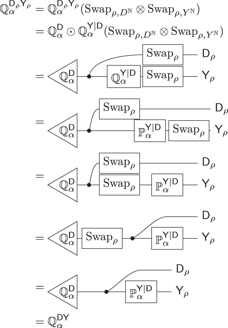
Proof
We apply absolute continuity of conditionals condition to show that
Note that by construction of
Equation (A26) defines a polynomial constraint on
Assuming (without loss of generality) we have
because the inequalities hold for the numerators and the denominators are equal. But then
because on the right side a smaller term in the sum receives more weight, a larger term receives less weight and all other terms are weighted equally.
Consider
and
then, by the same reasoning as before, we have
Analogous reasoning holds for
Suppose
On the other hand, by assumption, the set
By CIIR of the
We invoke precedent to establish that this also holds almost surely with respect to
and therefore, by
completing the proof.□
References
[1] Hernán MA, Taubman SL. Does obesity shorten life? The importance of well-defined interventions to answer causal questions. Int J Obesity. 2008 Aug;32(S3):S8–S14. https://www.nature.com/articles/ijo200882. 10.1038/ijo.2008.82Search in Google Scholar PubMed
[2] Hernán MA. Does water kill? A call for less casual causal inferences. Ann Epidemiol. 2016 Oct;26(10):674–80. http://www.sciencedirect.com/science/article/pii/S1047279716302800. 10.1016/j.annepidem.2016.08.016Search in Google Scholar PubMed PubMed Central
[3] Pearl J. Does obesity shorten life? Or is it the Soda? On non-manipulable causes. J Causal Inference. 2018;6(2):20182001. https://www.degruyter.com/view/j/jci.2018.6.issue-2/jci-2018-2001/jci-2018-2001.xml. 10.1515/jci-2018-2001Search in Google Scholar
[4] Hernán MA, Cole SR. Invited commentary: causal diagrams and measurement bias. Amer J Epidemiol. 2009 Oct;170(8):959–62. https://academic.oup.com/aje/article/170/8/959/145135. 10.1093/aje/kwp293Search in Google Scholar PubMed PubMed Central
[5] Shahar E. The association of body mass index with health outcomes: causal, inconsistent, or confounded? Amer J Epidemiol. 2009 Oct;170(8):957–58. 10.1093/aje/kwp292Search in Google Scholar PubMed
[6] Spirtes P, Scheines R. Causal inference of ambiguous manipulations. Philos Sci. 2004 Dec;71(5):833–45. https://www.cambridge.org/core/journals/philosophy-of-science/article/abs/causal-inference-of-ambiguous-manipulations/2A605BCFFC1A879A157966473AC2A6D2. 10.1086/425058Search in Google Scholar
[7] Pearl J. Causality: Models, reasoning and inference. 2nd ed. New York, NY: Cambridge University Press; 2009. 10.1017/CBO9780511803161Search in Google Scholar
[8] Heckerman D, Shachter R. Decision-theoretic foundations for causal reasoning. J Artif Intell Res. 1995 Dec;3:405–30. https://www.jair.org/index.php/jair/article/view/10151. 10.1613/jair.202Search in Google Scholar
[9] Dawid P. The decision-theoretic approach to causal inference. In: Causality. John Wiley & Sons, Ltd; 2012. p. 25–42. https://onlinelibrary.wiley.com/doi/abs/10.1002/9781119945710.ch4. 10.1002/9781119945710.ch4Search in Google Scholar
[10] Dawid P. Decision-theoretic foundations for statistical causality. J Causal Inference. 2021 Jan;9(1):39–77. 10.1515/jci-2020-0008Search in Google Scholar
[11] Lattimore F, Rohde D. Causal inference with Bayes rule. arXiv:191001510 [cs, stat]. 2019 Oct. http://arxiv.org/abs/1910.01510. Search in Google Scholar
[12] Lattimore F, Rohde D. Replacing the do-calculus with Bayes rule. arXiv:190607125 [cs, stat]. 2019 Dec. http://arxiv.org/abs/1906.07125. Search in Google Scholar
[13] de Finetti B. Foresight: its logical laws, its subjective sources. In: Kotz S, Johnson NL, editors. Breakthroughs in statistics: foundations and basic theory. Springer Series in Statistics. New York, NY: Springer; [1937] 1992. p. 134–74. 10.1007/978-1-4612-0919-5_10. Search in Google Scholar
[14] Lemeire J, Janzing D. Replacing causal faithfulness with algorithmic independence of conditionals. Minds and machines. 2013 May;23 (2):227–49. https://link.springer.com/article/10.1007/s11023-012-9283-1. 10.1007/s11023-012-9283-1Search in Google Scholar
[15] Meek C. Strong completeness and faithfulness in Bayesian networks. In: Proceedings of the Eleventh Conference on Uncertainty in Artificial Intelligence. UAI’95. San Francisco, CA, USA: Morgan Kaufmann Publishers Inc.; 1995. p. 411–8. http://dl.acm.org/citation.cfm?id=2074158.2074205. Search in Google Scholar
[16] Lindley DV, Novick MR. The role of exchangeability in inference. Ann Stat. 1981;9(1):45–58. https://www.jstor.org/stable/2240868. 10.1214/aos/1176345331Search in Google Scholar
[17] Rubin DB. Causal inference using potential outcomes. J Amer Stat Assoc. 2005 Mar;100(469):322–31. 10.1198/016214504000001880. Search in Google Scholar
[18] Imbens GW, Rubin DB. Causal inference for statistics, social, and biomedical sciences: an introduction. Cambridge: Cambridge University Press; 2015. https://www.cambridge.org/core/books/causal-inference-for-statistics-social-and-biomedical-sciences/71126BE90C58F1A431FE9B2DD07938AB. Search in Google Scholar
[19] Saarela O, Stephens DA, Moodie EEM. The role of exchangeability in causal inference. 2020 Jun. https://arxiv.org/abs/2006.01799v3. Search in Google Scholar
[20] Hernán MA, Robins JM. Estimating causal effects from epidemiological data. J Epidemiol Community Health. 2006 Jul;60(7):578–86. https://www.ncbi.nlm.nih.gov/pmc/articles/PMC2652882/. 10.1136/jech.2004.029496Search in Google Scholar PubMed PubMed Central
[21] Hernán MA. Beyond exchangeability: The other conditions for causal inference in medical research. Stat Methods Med Res. 2012 Feb;21(1):3–5. 10.1177/0962280211398037. Search in Google Scholar PubMed
[22] Greenland S, Robins JM. Identifiability, exchangeability, and epidemiological confounding. Int J Epidemiol. 1986 Sep;15(3):413–419. 10.1093/ije/15.3.413. Search in Google Scholar PubMed
[23] Banerjee AV, Chassang S, Snowberg E. Chapter 4 - Decision theoretic approaches to experiment design and external validity. In: Banerjee AV, Duflo E, editors. Handbook of economic field experiments. vol. 1 of Handbook of Field Experiments. North-Holland; 2017. p. 141–74. https://www.sciencedirect.com/science/article/pii/S2214658X16300071. 10.1016/bs.hefe.2016.08.005Search in Google Scholar
[24] Peters J, Bühlmann P, Meinshausen N. Causal inference by using invariant prediction: identification and confidence intervals. J R Stat Soc Ser B (Stat Methodol). 2016;78(5):947–1012. https://rss.onlinelibrary.wiley.com/doi/abs/10.1111/rssb.12167. 10.1111/rssb.12167Search in Google Scholar
[25] Guo S, Toth V, Schölkopf B, Huszar F. Causal de Finetti: On the identification of invariant causal structure in exchangeable data. Adv Neural Inform Proces Syst. 2023 Dec;36:36463–75. Search in Google Scholar
[26] Çinlar E. Probability and stochastics. New York, NY: Springer; 2011. 10.1007/978-0-387-87859-1Search in Google Scholar
[27] Liu Y, Price H. Ramsey and Joyce on deliberation and prediction. Synthese. 2020 Oct;197(10):4365–86. 10.1007/s11229-018-01926-8. Search in Google Scholar
[28] Constantinou P, Dawid AP. Extended conditional independence and applications in causal inference. Ann Stat. 2017;45(6):2618–53. http://www.jstor.org/stable/26362953. 10.1214/16-AOS1537Search in Google Scholar
[29] Kallenberg O. The basic symmetries. In: Probabilistic symmetries and invariance principles. Probability and its applications. New York, NY: Springer; 2005. p. 24–68. 10.1007/0-387-28861-9_2. Search in Google Scholar
[30] Eckles D, Bakshy E. Bias and high-dimensional adjustment in observational studies of Peer effects. J Amer Stat Assoc. 2021 Apr;116(534):507–17. 10.1080/01621459.2020.1796393. Search in Google Scholar
[31] Gordon BR, Zettelmeyer F, Bhargava N, Chapsky D. A comparison of approaches to advertising measurement: evidence from big field experiments at facebook. Rochester, NY: Social Science Research Network; 2018. ID 3033144. https://papers.ssrn.com/abstract=3033144. 10.2139/ssrn.3033144Search in Google Scholar
[32] Gordon BR, Moakler R, Zettelmeyer F. Close enough? A large-scale exploration of non-experimental approaches to advertising measurement. arXiv:220107055 [econ]. 2022 Jan. http://arxiv.org/abs/2201.07055. Search in Google Scholar
[33] Chickering DM. Learning equivalence classes of Bayesian-network structures. J Machine Learn Res. 2002;2(Feb):445–98. http://www.jmlr.org/papers/v2/chickering02a.html. Search in Google Scholar
[34] Uhler C, Raskutti G, Bühlmann P, Yu B. Geometry of the faithfulness assumption in causal inference. Ann Stat. 2013 Apr;41(2):436–63. http://arxiv.org/abs/1207.0547. 10.1214/12-AOS1080Search in Google Scholar
[35] Selinger P. A survey of graphical languages for Monoidal categories. In: Coecke B, editor. New structures for physics. Lecture Notes in Physics. Berlin, Heidelberg: Springer; 2011. p. 289–355. 10.1007/978-3-642-12821-9_4. Search in Google Scholar
[36] Fritz T. A synthetic approach to Markov kernels, conditional independence and theorems on sufficient statistics. Adv Math. 2020 Aug;370:107239. https://www.sciencedirect.com/science/article/pii/S0001870820302656. 10.1016/j.aim.2020.107239Search in Google Scholar
[37] Cho K, Jacobs B. Disintegration and Bayesian inversion via string diagrams. Math Struct Comput Sci. 2019 Aug;29(7):938–71. 10.1017/S0960129518000488Search in Google Scholar
[38] Fong B. Causal theories: a categorical perspective on Bayesian networks. arXiv: 13016201 [math]. 2013 Jan. http://arxiv.org/abs/1301.6201. Search in Google Scholar
[39] Okamoto M. Distinctness of the eigenvalues of a quadratic form in a multivariate sample. Ann Stat. 1973;1(4):763–65. https://www.jstor.org/stable/2958321. 10.1214/aos/1176342472Search in Google Scholar
© 2025 the author(s), published by De Gruyter
This work is licensed under the Creative Commons Attribution 4.0 International License.
Articles in the same Issue
- Research Articles
- Decision making, symmetry and structure: Justifying causal interventions
- Targeted maximum likelihood based estimation for longitudinal mediation analysis
- Optimal precision of coarse structural nested mean models to estimate the effect of initiating ART in early and acute HIV infection
- Targeting mediating mechanisms of social disparities with an interventional effects framework, applied to the gender pay gap in Western Germany
- Role of placebo samples in observational studies
- Combining observational and experimental data for causal inference considering data privacy
- Recovery and inference of causal effects with sequential adjustment for confounding and attrition
- Conservative inference for counterfactuals
- Treatment effect estimation with observational network data using machine learning
- Causal structure learning in directed, possibly cyclic, graphical models
- Mediated probabilities of causation
- Beyond conditional averages: Estimating the individual causal effect distribution
- Matching estimators of causal effects in clustered observational studies
- Ancestor regression in structural vector autoregressive models
- Single proxy synthetic control
- Bounds on the fixed effects estimand in the presence of heterogeneous assignment propensities
- Minimax rates and adaptivity in combining experimental and observational data
- Highly adaptive Lasso for estimation of heterogeneous treatment effects and treatment recommendation
- A clarification on the links between potential outcomes and do-interventions
- Review Article
- The necessity of construct and external validity for deductive causal inference