Beyond conditional averages: Estimating the individual causal effect distribution

1 Introduction

The main result of an epidemiological study is often summarized by an average treatment effect (ATE). Consequently, the ATE might (subconsciously) be interpreted as the causal effect for each individual, while individuals may react differently to exposures. These individual causal effects (ICEs) can be highly variable and may even have opposite signs [1,2]. The effect distribution within a (sub)population might be skewed, high in variability, or multimodal. Examples of ICE distributions for which the ATE is equal to − 15 are presented in Figure 1. One would like to go beyond mean estimation and draw inferences on the distribution of the ICEs. This inference involves the joint distribution of the potential outcomes of an individual that is not identifiable since the pair of potential outcomes under different levels of intervention cannot be observed simultaneously [3]. This fundamental problem of causal inference makes it impossible to estimate ICEs without making strong assumptions. Marginal causal effects can be characterized as generic functionals of the densities of potential outcomes [4]. Moreover, a difference in the shape of the potential outcome distributions can inform on some properties of the ICE distribution. For example, as we will explain further in this work, effect homogeneity can be ruled out when the variances of exposed and unexposed individuals are different in a randomized controlled trial (RCT). Under additional assumptions, the ICE distribution becomes identifiable and can be learned from the difference in shapes of the potential outcome distributions.

Figure 1

Examples of effect distributions where the (conditional) ATE equals − 15 . ICEs follow a Gaussian distribution with σ = 2 (a) and σ = 15 (b), respectively, a log-normal distribution ( μ = 4 , σ = 0.5 ), (c), or a Gaussian mixture distribution with p = 0.6 , μ 1 = − 31 , σ 1 = 10 , μ 2 = 9 , and σ 2 = 5 (d).

Nowadays, the variability in ICEs is typically studied by estimating conditional average treatment effects (CATEs), which equals the mean of the conditional ICE distribution given certain observed features. Standard causal inference methods can typically include covariates to account for such effect modification, e.g., strata-specific marginal structural models [5], and many machine learning (ML) algorithms have been proposed for flexible CATE estimation (see Caron et al. [6] for a detailed review). In this ML literature, a CATE based on many observed features is sometimes considered equivalent to the ICE [7]. In the ideal case of almost homogeneous conditional causal effects, such as for a subpopulation with the effect distribution shown in Figure 1(a), the CATE can be used to make treatment decisions for an individual. However, the CATE may not be informative enough when given the levels of the measured features the ICEs among the subpopulation are still highly variable, as shown in Figure 1(b) and (c). Despite accounting for many features of the patient, other and unknown features might modify the exposure effect so that in the subpopulation, the exposure is expected to harm some, while others benefit (e.g., Figure 1(d)). Despite the increasing number of covariates collected in epidemiological studies, significant effect modifiers may remain unmeasured so that the personalized CATE deviates from the personal ICE [8]. Therefore, (remaining) effect heterogeneity should be taken into account for decision-making [9–13].

In recent work, we have explained how CATE estimation using ML methods may be extended to additionally estimate the remaining conditional variance of the ICE assuming conditional independence of the individual effect and the potential outcome under no exposure, a causal assumption [8]. The conditional ICE distribution is only identified by this conditional variance and the CATE when assuming (conditionally) Gaussian-distributed effects. Under the conditional independence assumption, the Gaussianity of the effect is not a causal assumption because it could be verified with sufficient observed data. In this work, we shift focus from the (conditional) ICE variance to the (conditional) ICE distribution without assuming the shape of the effect distribution. We will explain under what assumptions the (conditional) ICE distribution becomes identifiable so that latent variable models may be used to estimate the distribution. We will present a semi-parametric linear mixed model (LMM) to estimate the (conditional) ICE distribution when the assumptions apply and discuss the complications in estimation due to the heterogeneity of the effect of confounders on the outcome.

First, we will introduce our notation and framework to formalize individual effect heterogeneity in Section 2. In Section 3, we will review the literature related to ICE and illustrate how and under which assumptions the ICE distribution can be identified from an RCT and observational data, respectively. Subsequently, the semi-parametric causal mixed models and possible methods to fit these models are presented in Section 4. In Section 5, the Framingham heart study (FHS) is considered to illustrate how the reasoning presented in this work could be used in practice. The modeling considerations are discussed in detail. Finally, we reflect on the work’s importance, limitations, and future research in Section 6.

2 Notation and framework

Probability distributions of factual and counterfactual outcomes are defined in the potential outcome framework [14,15]. Let Y i and A i represent the (factual) stochastic outcome and the random exposure assignment level of individual i . Let Y i a equal the potential outcome (counterfactual when A i ≠ a ) under an intervention on the exposure to level a . We thus assume deterministic potential outcomes so that each level of exposure corresponds to a specific outcome for each individual (but its value typically differs between individuals) [16,17].

We will consider only two exposure levels, a ∈ { 0 , 1 } , with 0 indicating no exposure. The ICE of an arbitrary individual i from the population of interest is defined on the additive scale as Y 1 − Y 0 [18, Chapter 1].

Throughout this work, we will assume causal consistency, implying that potential outcomes are independent of the assigned exposure levels of other individuals (no interference) and that there are no different versions of the exposure levels [19].

This definition of causal consistency is also referred to as the stable unit treatment value assumption [20, Assumption 1.1]. Furthermore, we will assume that for all levels of measured features X , the probability of exposure is bounded away from 0 and 1, known as positivity [18, Chapter 3].

Next, we will introduce a structural model and random variables necessary to formalize the relevant causal relations and joint distribution of potential outcomes. The variability in exposure assignment A among individuals is accommodated by the variable N A . Individuals can have different potential outcomes under no exposure, Y 0 , represented by a population average θ and an individual-specific deviation N Y . The latter random variable results in dependence between Y 0 and Y 1 . In addition, ICE is equal to the population average effect τ and an individual random effect deviation U 1 . We describe the cause–effect relations with a structural causal model (SCM), which is commonly used in the causal graphical literature (see, e.g., Pearl [21, Chapter 1.4] and Peters et al. [22, Chapter 6]), to formalize the system behind the observed outcomes. Instead, we include both individual effect modifiers U 1 and the latent common cause of potential outcomes N Y to describe the two potential outcomes of an individual jointly. An SCM as presented in this article is therefore a union of the SCM for observations ( A = a ), and the so-called intervened SCMs for all possible d o ( A = a ) . It consists of a joint probability distribution for ( N A , N Y , U 1 ) and a structural assignment f A ^[1] such that

Note that U 1 i can still depend on N Y i , so that SCM (1) is a saturated model and does not impose any restrictions. For example, consider a system where Y i 1 = 2 Y i 0 = 2 θ + 2 N Y i , then τ = θ and U 1 i = N Y i . Although no other observed features X are present in the SCM (1), U 1 i and N Y i can depend on X . Later in this work, the SCM (1) will be reparamaterized by including observed features X . The joint distribution of U 1 i and N Y i is not identifiable without additional assumptions and will play a vital role in this work. The SCM (1) also describes the data-generating mechanism since Y i A i = Y i .

There exists confounding when N A i ⫫̸ N Y i , U 1 i , so that A ⫫̸ Y 0 , Y 1 . For observational data, many causal inference methods require the absence of unmeasured confounding, i.e., observed features X should contain a sufficient adjustment set, and the observed features should not contain colliders [23]. Then, Y 0 , Y 1 ⊥ ⊥ A ∣ X , referred to as conditional exchangeability [18, Chapter 3], and the marginal distributions of the potential outcomes are identified by the observed conditional distributions.

As discussed in Section 1, causal effect heterogeneity is often addressed by studying the CATEs in subpopulations defined by measured features X (e.g., sex, age, or co-morbidity) that may be effect modifiers so that Y 1 − Y 0 ⫫̸ X . The CATE estimand equals E [ Y 1 − Y 0 ∣ X = x ] , so that with the parameterization in SCM (1), the CATE for X = x is equal to τ + E [ U 1 ∣ X = x ] . Under Assumptions 1–3 the CATE is identifiable, and using causal methods such as inverse probability of treatment weighting (IPTW) for adjustment, unbiased CATE estimates can be obtained [18, Chapter 2]. Note that conditioning on X can thus have two purposes: adjusting for confounding to obtain conditional exchangeability and explaining part of the effect heterogeneity. For example, when studying effect heterogeneity from a randomized experiment, one does not have to adjust for X for exchangeability to hold but can condition to study the CATEs for different levels of X .

The CATE equals the mean of the conditional ICE distribution, P ( Y 1 − Y 0 ≤ y ∣ X = x ) . The ICE distribution is the estimand of interest in this work. In contrast to the CATE, the ICE distribution itself can only be identified from cross-sectional data after assuming how Y 1 − Y 0 depends on Y 0 . We will show in Section 3 that a sufficient assumption for identifiability of the ICE distribution (when Assumptions 1–3 apply) would be conditional independence of the ICE and Y 0 .

For the parameterization of the cause–effect relations in terms of SCM (1), this is equivalent to assuming U 1 ⊥ ⊥ N Y ∣ X = x . Assumption 4 means that after taking into account features X , the potential outcome under no exposure is not informative for the value of the individual effect. The assumption could, for example, apply when the causal effect of a treatment is the result of a catalytic reaction mechanism. Then, the ICE of exposure depends on the amount of a catalyst present for an individual, while conditionally, on features X , this amount of catalyst is not associated with Y 0 . Post et al. [8] presented an example of the effect of an antiplatelet medicine, which depends on the conversion to an active metabolite accomplished by a specific enzyme. Heterogeneity in ICE results from heterogeneity in the amount of enzyme present. After adjusting for features that are related to the amount of enzyme, the actual amount of enzyme does not inform on Y 0 , so that Y 1 − Y 0 ⊥ ⊥ Y 0 ∣ X .

Realize that Assumption 4 is violated when there exists a feature that, despite conditioning on X , affects both Y 1 − Y 0 and Y 0 and is not adjusted for. Moreover, it is good to realize that when Assumption 4 applies, then Y 1 Y 0 will generally not be independent of Y 0 given X . In our work, we are interested in the causal effect defined as the difference of potential outcomes, and thus, Assumption 4 involves that difference. When the focus is on another contrast of potential outcomes, an assumption similar to 4 but involving that contrast will be required.

3 Identifiability of the ICE distribution

As a result of the fundamental problem of causal inference, studying properties of the conditional ICE distribution other than the CATE (which equals the mean) received less attention in the literature. For binary outcomes Y and exposures A , the ICE distribution can be described by the probability of necessity (PN, i.e., P ( Y 0 = 0 ∣ A = 1 , Y = 1 ) ), the probability of sufficiency (PS, i.e., P ( Y 1 = 1 ∣ A = 0 , Y = 0 ) ), and the probability of necessity and sufficiency (PNS, i.e., P ( Y 1 = 1 , Y 0 = 0 ) ) that is also referred to the probability of benefit [24]. For binary exposures and outcomes, the PN is identifiable under a monotonic effect assumption ( Y 1 ≥ Y 0 ) [21]. For the case with multiple causes that could affect each other, similar monotonicity assumptions have been presented to identify the posterior total and direct causal effects [25]. Furthermore, again for binary exposures, under the assumption of monotonic incremental treatment effect (i.e., 0 ≤ Y 1 − Y 0 ≤ 1 ), the PS has been shown to be identifiable for ordinal outcomes [26]. Assuming the absence of unmeasured confounding, bounds on the PN, PS, and PNS obtained from combined experimental and observational data have been presented [24], and their applicability in practice was shown [27]. Similarly, to study the conditional (on covariates) ICE distribution, conditional bounds of the PNS can be estimated [12]. When combining experimental and observational data, bounds have also been presented for multi-valued outcomes and exposures [28]. Moreover, for multi-valued outcomes, binary exposures, and when only using experimental data, a consistent estimator for the bounds of the treatment benefit ratio (TBR) [29] and a method to estimate corresponding confidence intervals have been presented [30]. The TBR is equal to P ( Y 1 − Y 0 > 0 ) when an increase in the outcome is beneficial and equal to P ( Y 1 − Y 0 < 0 ) when a decrease is beneficial. Bounds have also been presented for the treatment harming rate (THR, P ( Y 1 − Y 0 < 0 ) when an increase in the outcome is beneficial), also known as the fraction negatively affected [31,32]. These bounds can be improved by restricting the range of the Pearson correlation coefficient between potential outcomes [33]. Recently, a method to estimate lower confidence limits for quantiles of the ICE distribution from experimental data has been proposed for general outcomes and binary exposures, allowing inference on the proportion of units with ICEs passing any threshold [34]. Su and Li [34] have also presented a sensitivity analysis to apply the methodology to observational data and quantify the effect of unmeasured confounding. Furthermore, ideas from conformal inference have been leveraged to derive individualized prediction intervals for ICEs with 1 − α marginal coverage guarantees assuming the absence of unmeasured confounding [35]. More specifically, Lei and Candes [35] presented conformalized counterfactual inference to derive prediction intervals for both potential outcomes given the observed features. Moreover, they presented both exact and inexact methods to construct intervals for the conditional ICE and demonstrated with numerical experiments that the exact methods are conservative. To robustify the method in cases where unmeasured confounding might exist, sensitivity analyses have been proposed [36,37]. Finally, extensions focus on conditional rather than marginal coverage guarantees [38,39].

Besides the non-parametric approaches, non-verifiable assumptions on the joint distribution of the potential outcomes ( Y 0 , Y 1 ) have been made by using latent variable models to estimate the TBR [32,40,41] and the ICE distribution [42]. There exists work in which it is assumed that Y 1 ⊥ ⊥ Y 0 given features X = x , while Y 1 − Y 0 given X = x is assumed to follow a Gaussian mixture distribution [42] or is degenerate [32]. Yin et al. [40] assumed Assumption 4 but restricted the conditional ICE distribution given X = x to be Gaussian. Instead of a direct assumption on the joint distribution of the potential outcomes, Laubender et al. [41] assumed that next to Y , a biomarker is observed that is a surrogate of Y 1 + Y 0 and by assuming that Y 0 , Y 1 and the biomarker follow a multivariate Gaussian distribution, the conditional TBR becomes identifiable.

In this section, we discuss the non-identifiability of the ICE as a result of the fundamental problem in more detail and explain why Assumption 4 can result in identifiability. To build intuition, we begin by showing how the fundamental problem of causal inference results in the non-identifiability of the conditional variance.

4 Causal mixed models

We continue by focusing on fitting the unknown F Y ∣ A = 1 , X = x , and F Y ∣ A = 0 , X = x from data. Under Assumptions 1–3, Y ∣ A = a , X = x is equal in distribution to Y a ∣ X = x ; thus, by SCM (1),

where f Y 0 ( x ) = θ + E [ N Y ∣ X = x ] , f Y 1 ( x ) = τ + E [ U 1 ∣ X = x ] and the distributions F N Y x ( x ) and F U 1 x ( x ) can depend on x but have zero mean for all x . If N Y x does not depend on X , then f Y 0 ( X ) is the prognostic score of Y 0 since Y 0 ⊥ ⊥ X ∣ f Y 0 ( X ) [44]. If U 1 x is also independent of X , then { f Y 0 ( X ) , f Y 1 ( X ) } is the prognostic score of Y 1 .

Note that ∫ f Y 1 ( x ) d F X ( x ) equals the ATE τ , f Y 1 ( x ) equals the CATE for X = x , and the ICE for individual i equals f Y 1 ( X i ) + U 1 x i .

The distribution of ( U 1 x , N Y x ) in (6) and the functional forms of f Y 0 and f Y 1 are unknown. One can try to fit the observed data using a (flexible) mixed model with a random exposure effect Z 1 ,

where the distributions F ε ( x ) and F Z 1 ( x ) can depend on x but have zero mean for all x , e.g., heteroskedastic residuals, but we assume Z 1 i ⊥ ⊥ ε i ∣ X i . At this point, the latter independence is thus the only restriction of the associational model (7). Note that the functions f Y 0 and f Y 1 , and the distributions of U 1 x and N Y x follow from SCM (1), while the functions β 0 and β 1 , and the distributions of Z 1 and ε are part of the statistical model that is fitted to the observed data. If Assumptions 1–4 apply, and model (7) is well specified^[3], then the distribution of β 1 ( X ) + Z 1 ∣ X = x equals the distribution of Y 1 − Y 0 ∣ X = x by Proposition 3. There is a lot of research on non-parametric (ML) methods to estimate the functionals β 0 and β 1 [8]. In the remainder of this article, we will focus on estimating the (conditional) distributions of ε and Z 1 .

4.2 Example of ICE distribution estimation

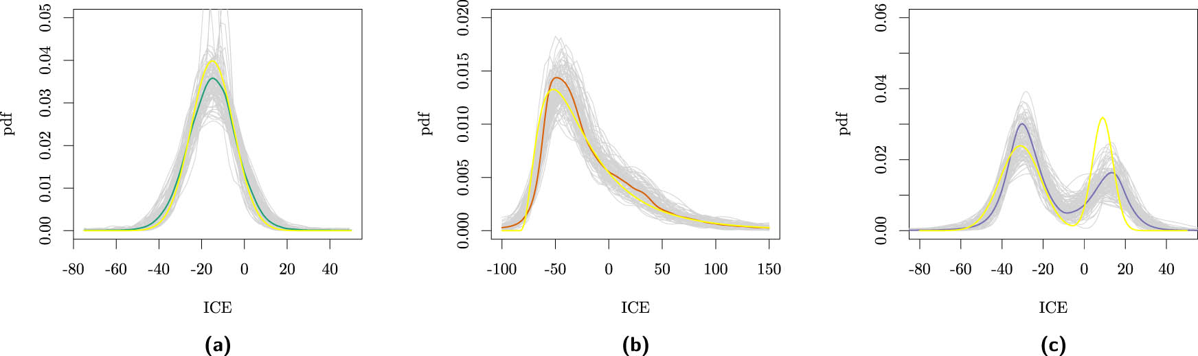
To demonstrate the use of a causal mixed model, we will next consider a simple example with data simulated for 1,000 individuals using equation (6) with f Y 0 ( x ) = θ 0 + x θ 1 , while N Y x , U 1 x ⊥ ⊥ A and U 1 x ⊥ ⊥ N Y x , N Y x is Gaussian-distributed, and U 1 x follows a Gaussian distribution, a log-normal distribution, or a mixture of two Gaussians, respectively. For simplicity, we will assume that only one binary confounder exists that is no modifier (on the additive scale, f Y 1 ( x ) = τ ). Details on the parameters used can be found in the caption of Figure 2.

Figure 2

Estimated Z 1 distributions for 100 simulations for underlying ICE distributions τ + U 1 x , where τ = − 15 , U 1 x ∼ N ( 0 , 1 0 2 ) (left), or U 1 x ∼ LN ( 4 , 0.5 2 ) − exp ( 4 + 0.5 0.5 2 ) (middle) or a two-component Gaussian mixture such that with probability p = 0.6   U 1 ∼ N ( − 16 , 1 0 2 ) , and otherwise, U 1 ∼ N ( 24 , 5 2 ) (right). The actual density for τ + U 1 (yellow) and the mean of the estimated Z 1 densities (black) are presented. Data for individuals were simulated using equation (6), where N Y x ∼ N ( 0 , 50 ) , f Y 0 ( x ) = θ 0 + x θ 1 , f Y 1 ( x ) = τ , where θ 0 = 120 and the effect of the confounder was θ 1 = 5 . The confounder X had the value − 0.3 with probability 0.7 and value 0.7 with probability 0.3 and thus a zero mean. The probability of exposure equaled logit ( − 3 + 3 X i ) for individual i . Finally, N Y x , U 1 x ⊥ ⊥ A and U 1 x ⊥ ⊥ N Y x .

We will model the ICE distribution with a Gaussian mixture that we fit using the Bayesian method with an upper bound for the number of components (discussed in Section 4.1) since this one-step approach can be easily implemented in both SAS and R. Moreover, since we are interested in estimating the entire distribution of the ICE, a Bayesian method has the advantage that (pointwise) uncertainty quantification of the ICE density can be directly obtained. On the contrary, when using a frequentist approach, the uncertainty of the density should be derived from the uncertainty in the model parameters.

We model the observed data as

(8) Y i = β 0 + X i β X + A i Z 1 i + ε i ,

where Z 1 i follows a K -dimensional Gaussian mixture distribution with mixing probabilities p , component means μ , and component variances τ 2 (i.e., Z 1 i ∼ GM ( p , μ , τ 2 ) ), ε i ∼ N ( 0 , σ 2 ) , Z 1 i ⊥ ⊥ ε i , and Z 1 i , ε i ⊥ ⊥ X i . For 1 ≤ j ≤ K , the recommended non-informative priors [56, Chapter 22]

(9) μ j , β 0 , β X ∼ N ( 0 , 1 0 5 ) ,

(10) τ j , σ ∼ Uni [ 0 , 100 ] ,

and the weakly informative prior

(11) p ∼ Dir ( α , … , α ) ,

are used. When (8) is well specified and Assumptions 1–4 apply, by Proposition 3, P ( Y 1 − Y 0 ≤ y ) equals P ( Z 1 ≤ y ) . Since Z 1 is a univariate random variable, K = 5 should suffice to capture important characteristics, i.e., skewness and multi-modality, of the ICE distribution as suggested elsewhere [51, Section 22.4]. As we do not have prior knowledge about the ICE distribution, we should be careful not to select a too small α that would favor distributions closer to a normal distribution via the weakly informative prior. The prior distribution of the number of prominent components, i.e., p j ∈ p : p j > 0.10 , for different levels of α is presented in Figure A1. Here, we use α = 0.5 , giving rise to Jeffreys prior for the labeling distribution [53]. In this work, we use PROC MCMC in SAS to perform the Bayesian analysis. During every Monte-Carlo iteration, for each individual, a latent modifier is sampled from the Gaussian mixture based on the parameters sampled for that specific iteration. Finally, the posterior Z 1 distribution is presented using a kernel density estimation of all sampled Z 1 . The posterior distributions of Z 1 are presented for 100 simulated datasets and different underlying ICE distributions in Figure 2. In expectation (black lines), the characteristics of the ICE distribution are well recovered. For illustration, for an arbitrary dataset, the kernel density estimates of the sampled Z 1 per Markov chain Monte Carlo (MCMC) iteration (gray) are presented together with the posterior distributions of Z 1 (colored) and the underlying Y 1 − Y 0 distribution (yellow) as Figure A2 (a)–(c) in Appendix.

The mean values of the posterior means and the coverage of the Bayesian credible sets are presented in Table 1 for P ( Z 1 > 0 ) and the quantiles of the distribution of Z 1 . For these datasets with 1,000 individuals, the averages of the posterior means for all three ICE distributions are close to the actual levels of P ( Y 1 − Y 0 > 0 ) and the quantiles of the ICE distribution considered. Note that P ( Y 1 − Y 0 > 0 ) is equal to the TBR if higher outcomes are beneficial and equal to the THR otherwise. Furthermore, the coverages of the Bayesian credible sets for this sample size are pretty close to 0.95, although for the non-Gaussian U 1 distributions, the coverage tends to be slightly lower.

Table 1

Actual values of P ( Y 1 − Y 0 > 0 ) and the 5, 25, 50, 75, and 95% quantiles for the different ICE distributions

	Actual value			Average posterior means			Coverage credible sets
	(a)	(b)	(c)	(a)	( b ) *	(c)	(a)	( b ) *	(c)
P ( Y 1 − Y 0 > 0 )	0.07	0.27	0.39	0.08	0.27	0.36	0.95	0.94	0.90
α 0.05	− 31.44	− 68.04	− 44.83	− 33.48	− 71.96	− 45.58	0.90	0.94	0.90
α 0.25	− 21.74	− 51.21	− 33.10	− 21.72	− 50.19	− 33.13	0.92	0.89	0.91
α 0.5	− 15	− 30.51	− 21.33	− 14.88	− 30.31	− 18.71	0.95	0.89	0.90
α 0.75	− 8.25	2.86	7.41	− 8.14	4.14	6.83	0.96	0.93	0.88
α 0.95	1.44	89.60	14.75	3.42	90.50	15.90	0.97	0.89	0.86

For these characteristics, the average of the posterior means, each estimated on 1,000 individuals, and the coverage of the 95% Bayesian credible sets, based on the 100 simulations, are presented.

In practice, the model itself should be validated after verifying the proper convergence of the Markov chains. The causal Assumptions 1, 3, and 4 cannot be verified, but the associational model can be validated using the observational data, as we will elaborate on in Section 5. It is essential to realize that when Assumption 4 is violated, the ICE distribution is not identified by the Z 1 distribution. If Y 0 and Y 1 − Y 0 are negatively correlated, the variability in the ICE distribution will be underestimated by the variability in the Z 1 distribution. In Figure 3 (a), this is illustrated for data simulated from the system discussed in this section, but now the correlation between N Y x and U 1 x is ρ = − 0.75 . Similarly, for ρ = 0.75 , Y 0 and Y 1 − Y 0 are positively correlated, and the variability of the ICE distribution is overestimated (Figure 3 (b)).

Figure 3

Estimated Z 1 distributions for 100 simulations for underlying ICE distributions τ + U 1 x , where τ = − 15 and ( U 1 x , N Y x ) is bivariate normal distributed with zero means, variance 1 0 2 and 50, respectively, and correlation ρ = − 0.75 (a) or ρ = 0.75 (b). The actual density for τ + U 1 x (yellow) and the mean of the estimated Z 1 densities (black) are presented. Data for individuals were simulated using equation (6), where N Y x ∼ N ( 0 , 50 ) , f Y 0 ( x ) = θ 0 + x θ 1 , f Y 1 ( x ) = τ , where θ 0 = 120 , and the effect of the confounder was θ 1 = 5 . The confounder X had the value − 0.3 with probability 0.7 and value 0.7 with probability 0.3 and thus a zero mean. The probability of exposure equaled logit ( − 3 + 3 X i ) for individual i and N Y x , U 1 x ⊥ ⊥ A .

4.3 Confounding-effect heterogeneity

As stated in equation (6), the distribution of N Y x and U 1 x can depend on X . Then, also ε and Z 1 should depend on X to have a well-specified model (7). This is particularly important when the distributions of N Y x and U 1 x depend on confounders since the fitted distribution of Z 1 will represent the difference in the shape of the conditional distribution between exposed and unexposed individuals. Thus, when we do not appropriately adjust for confounders, Z 1 will never represent the U 1 x distribution.

For causal inference from observational data, it is often necessary to adjust for features so that Assumption 3 applies. If the interest is in the ATE, we in principle only need to take into account the confounder’s effect on the outcome’s mean, i.e., we need to adjust for X so that

E [ Y a ∣ X = x ] = E [ Y ∣ X = x , A = a ] .

However, if one is interested in the ICE distribution, then it is necessary to consider the effect of the confounder on the entire distribution of the outcome, i.e., adjust for X so that Assumption 3 applies and

F Y a ∣ X = x ( y ) = F Y ∣ X = x , A = a ( y ) .

Otherwise, a difference in (the shape of the) distribution between the exposed and unexposed individuals can be caused by the non-exchangeable confounders. Then, the estimated distribution of Z 1 in (7) is a mixture of the heterogeneity in the effects of the confounders and the exposure effect. By verifying whether the proposed distribution fits well in sub-samples grouped by the levels of the confounders, one can decide whether accounting for the effect on the mean is sufficient. The effects of a confounder on the outcome of different individuals might follow a non-degenerate distribution. If so, then confounding-effect heterogeneity exists. An (extreme) example of confounding-effect heterogeneity is the case where only the outcome of a proportion of individuals is affected by the confounder [57]. For another example, let us again consider the example presented in Section 4.2, but now we let N Y x depend on X so that N Y x ∣ X = 0.7 and N Y x ∣ X = − 0.3 are Gaussian-distributed with variance 50 and 50 + 1 0 2 , respectively. Then, model (8) is misspecified, and as a result, the variability of the ICE distribution is underestimated, as presented in Figure 4(a). The variability is underestimated since among the unexposed X = − 0.3 is more prevalent than among the exposed.

Figure 4

Estimated Z 1 distributions after fitting model (8) (a) or (12) (b) for 100 simulations for underlying ICE distributions τ + U 1 x , where τ = − 15 and U 1 x ∼ N ( 0 , 10 2 ) . The actual density for τ + U 1 (yellow) and the mean of the estimated Z 1 densities (black) are presented. Data for individuals were simulated using equation (6), where N Y x Gaussian-distributed, f Y 0 ( x ) = θ 0 + x θ 1 , f Y 1 ( x ) = τ , where θ 0 = 120 and the effect of the confounder was θ 1 = 5 . The confounder X had the value − 0.3 with probability 0.7 and value 0.7 with probability 0.3 and thus a zero mean. The variance of N Y x was equal to 50 for X = 0.7 and 50 + 1 0 2 for X = − 0.3 and the probability of exposure equaled logit ( − 3 + 3 X i ) for individual i and N Y x , U 1 x ⊥ ⊥ A .

In the case of confounding-effect heterogeneity, the distribution of ε in (7) should depend on the level of the confounders. Indeed, when model (8) is extended as

(12) Y i = β 0 + X i β X + X ˜ i Z X i + A i Z 1 i + ε i ,

where X ˜ i equals 0 if X i = 0.7 and 1 otherwise and Z X i ∼ N ( 0 , τ X 2 ) , the model is well specified and the ICE distribution can be accurately represented with the Z 1 distribution, as presented in Figure 4 (b).

Similarly, the Z 1 distribution does not represent the ICE distribution when the N Y x distribution cannot be approximated with the proposed distribution of ε . Then, the Z 1 distribution obtained by fitting model (7) is a mixture of U 1 x and the deviation of the distribution of N Y x from the proposed distribution for ε , such that the model will better fit the data of the exposed individuals. This problem can be verified by evaluating the fit to the data of the unexposed individuals and might be solved using a more flexible distribution for ε .

5 Case study: the FHS

In this section, we consider heterogeneity in the effect of non-alcoholic fatty liver disease on cardiac structure and function, as studied by Chiu et al. [58] in the FHS population. We will work with a subset of the FHS third-generation and offspring cohorts ( n = 2352 ) . To illustrate our proposed method, we focus on the effect of hepatic steatosis (fatty liver disease) on the left ventricular filling pressure (LVFP), a clinical precursor to heart failure. Hepatic steatosis was defined as having a liver phantom ratio (measured fat attenuation in three areas of the liver divided by a phantom calibration control) exceeding 0.33. It was estimated to increase the expected LVFP by 0.46, with a 95% confidence interval equal to (0.26, 0.65), after adjustment for confounding [58].

The sample standard deviation of the LVFP equals 2.27 for individuals exposed to hepatic steatosis and only 1.74 for those who were not. This difference might be the result of causal effect heterogeneity. As the Bayesian analysis discussed in Section 4.2 is computationally intensive, we started by fitting a traditional Gaussian LMM to investigate which candidate confounders affected the estimated mean or variance of the effect of hepatic steatosis on LVFP. Confounders accounted for in the original study were age, sex, smoking, alcohol use, diabetes, systolic blood pressure (SBP), use of antihypertensive medication (HRX), use of lipid-lowering medication, total cholesterol, high-density lipoprotein cholesterol, triglycerides, and fasting glucose. The relevant confounders were age, sex, diabetes, SBP, and HRX (details can be found in Section E of Appendix).

In this case study, our focus is on the population ICE distribution; thus, we do not consider modifiers that are no confounders. We have fitted the model

where Z 1 i ∼ GM ( p , μ , τ 2 ) , with K = 5 , ε i ∼ GM ( p ˜ , μ ˜ , τ ˜ 2 ) with K ˜ = 3 while restricting E [ ε i ] = 0 , and Z i ⊥ ⊥ ε i . We believe that it was appropriate to model the residual (and thus Y ∣ A = 0 , X = x ) with a more flexible distribution as we do not condition on any features other than adjusting for confounders such that the distribution is expected to be more complex than Gaussian. This is important since misspecification of the residual distribution will affect the estimated distribution of Z 1 as explained at the end of Section 4.3. Alternative flexible error distributions have been presented in the literature [42,59,60].

The model was fitted using the Bayesian method discussed in Section 4.2. The initial values for the parameters in the Markov chain were based on the final Gaussian LMM used to select the confounders and can be found in Table A6 in Appendix. Per chain, we have used 100,000 burn-in iterations, followed by 500,000 MCMC iterations. We have used a thinning rate of 100 to save computer memory space. In total, 5 chains, each contained 5,000 (thinned) MCMC iterations that were saved. Each chain was split into two pieces, and we investigated the convergence of the X i β XA T + Z 1 i distribution for the first unexposed individual in the dataset. Convergence of the Markov chains was supported by an estimated R-hat convergence diagnostic, as defined by Vehtari et al. [61], equal to R ˆ = 1.01 , and the estimated bulk and tail effective sample sizes equal to 2.5 × 1 0 4 and 1.8 × 1 0 4 , respectively. The trace plot for the X i β XA T + Z 1 i of this (and another) unexposed individual can be found in Figure A3 in Appendix.

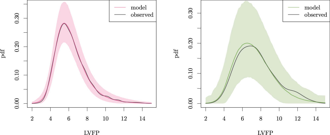
We should ensure that the model accurately fits the observed data to draw inferences on the ICE distribution. To validate the model, we study the posterior predictive distribution of the LVFP for both the exposed and unexposed individuals ( Y ∣ A = a ), as presented in Figure 5. The distribution of the outcomes of the unexposed individuals ( Y ∣ A = 0 ) is well fitted using a three-component Gaussian mixture residual. Furthermore, a five-component Gaussian mixture for the individual effect distribution is flexible enough to fit well the observations of the exposed individuals ( Y ∣ A = 1 ).

Figure 5

Posterior predictive distribution of the LVFP for model (13), with corresponding 95% BCIs and the kernel density of the observed data for unexposed (left) and exposed individuals (right).

As shown in Table 2, the standard deviation of the LVFP is higher for individuals who are either older, female, have diabetes, have higher blood pressure, or use HRX for both exposure groups. In Section 4.3, we have explained how confounding-effect heterogeneity can affect the distribution of Z 1 . The validation of the fit of the Y ∣ X = x distribution for all dichotomized levels of the confounders ( > median value) is thus a crucial part of the analysis. The posterior predictive distributions in all groups of dichotomized confounders are presented in Section F.1 of Appendix. Overall, we conclude that significant confounding-effect heterogeneity seems to be absent. In Section 5.1, we demonstrate how a model may be fitted when confounding-effect heterogeneity is present.

Thus, model (13) does appropriately describe the observed conditional distributions. The ICE distribution is only identifiable in the absence of other confounders and when the dependence of Y 1 − Y 0 and Y 0 is known. Under Assumptions 1–4, the ICE distribution is identified by the distribution of Z 1 , which estimate is presented in Figure 6 (solid line). The ATE has a posterior mean of 0.43 with a 95% Bayesian credible interval (BCI) equal to (0.23, 0.63). The ATE is thus similar to the effect found by Chiu et al. [58] and to an ATE estimate of 0.44, with a 95% confidence interval of (0.28, 0.60), obtained using IPTW. The added value of this analysis is inference on other properties of the ICE distribution. For example, 20.6% (BCI: 8.9%, 33.6%) of the individuals were estimated to have a harming effect of hepatic steatosis on the LVFP that is larger than twice the ATE ( P ( ICE > 2 × 0.43 ) ). The ATE should thus not be used as an individual effect measure.

Figure 6

Posterior distribution of the effect of hepatic steatosis on the LVFP using model (13) (solid line) and pointwise 95% BCIs. Moreover, distributions obtained when either adjusting for confounding-effect heterogeneity, using a Gaussian residual or a Gaussian LMM, respectively, are presented for comparison (Section 5.1).

5.1 Sensitivity analysis

We performed a sensitivity analysis by extending model (13) with confounder-specific residual variances to demonstrate how one could try to adjust for confounding-effect heterogeneity. We have fitted the model

(14) Y i = β 0 + X i β X T + ( X i β XA T + Z 1 i ) A i + δ i , δ i = ε i + X ˜ i Z X i T ,

where again Z 1 i ∼ GM ( p , μ , τ 2 ) , with K = 5 , ε i ∼ GM ( p ˜ , μ ˜ , τ ˜ 2 ) with K ˜ = 3 and E [ ε i ] = 0 , and now, Z X i are zero-mean Gaussian-distributed, while all latent variables are independent. Dichotomized versions of the confounders ( > median) are presented by X ˜ i . This way, one corrects for the shift in mean and the increased variance in the subpopulations with particular values for the confounders. Again, the fit of this distribution to the observed data should be verified. When this model is not appropriate, one could decide to extend the model further by modeling part of the Z X with a mixture of Gaussians instead of the Gaussian distribution.

The posterior predictive checks in the different exposure and confounder strata can be found in Section F.2 of Appendix. The minor differences between the posterior predictive distribution and the observed distribution presented in Section F.1 of Appendix became even smaller. The ATE has a posterior mean of 0.38 (95% BCI: 0.19, 0.56), and the posterior mean of the P ( ICE > 2 × 0.43 ) equals 20.4% (8.9, 34.0). These estimates were (as expected) very similar to the ones obtained by fitting model (13), and the estimated distribution is also presented in Figure 6.

We want to emphasize that all latent variables must be modeled with a distribution that is flexible enough to fit the observed outcomes accurately. For comparison, we have also presented the estimated ICE distribution when modeling the residual with a Gaussian distribution without adjusting for confounding-effect heterogeneity (ATE equals 0.42 (0.17, 0.69)) and P ( ICE > 2 × 0.43 ) equals 12.5% (6.5, 21.8) in Figure 6. However, in this case, the model for Y ∣ A = 0 is misspecified as presented in Figure A15 in Appendix F.3. When using a Gaussian LMM without adjusting for confounding-effect heterogeneity (ATE equals 0.41 (0.17, 0.65), and P ( ICE > 2 × 0.43 ) equals 36.7% (29.8, 43.7)) also the model for Y ∣ A = 1 seems misspecified as presented in Figure A16 in Appendix F.4.

Figure A1

Distribution of the number of p j ∈ p : p j > 0.10 when p ∼ Dir ( α , α , α , α , α ) for α = 1 5 (a), 1 2 (b), and 1 (c).

6 Discussion

Methods for causal inference have rapidly evolved over the past decades. As a result, making causal claims from observational studies became more common, relying on expert knowledge to back up the untestable identifiability assumption of conditional exchangeability. However, such methods focus on learning (conditional) ATEs rather than effect distributions. Therefore, the results are only informative at the level of an individual when (remaining) effect heterogeneity is low. In this work, we have presented an identifiability assumption that suffices to move from the (conditional) ATE to quantification of the (conditional) distribution of causal effects.

In the case of effect heterogeneity, exposure (or absence thereof) increases variability in the outcome as individuals respond differently. When the common causal Assumptions 1–3 apply and additionally (conditional) independence of the ICE and the potential outcome under no exposure (Assumption 4) can be assumed, inference on the ICE distribution can be drawn from cross-sectional data. The joint distribution of potential outcomes should be linked to the law of observations, which can be learned from the data. Then, deviations from the (C)ATE could be quantified. In case of serious deviations, the shape of the (conditional) ICE distribution can inform about the remaining heterogeneity of the exposure effect. It may illustrate that there is still a severe lack of understanding of the exposure effect as the presence of unmeasured modifiers is considerable. The distribution of the unmeasured modifiers may differ across populations, so estimated ICE distributions could be helpful in the understanding of differences in causal effects [62].

In contrast to the well-established models to estimate CATEs (e.g., [63] and [64]), the focus of the methods presented in this article is inference on the distribution that quantifies remaining effect heterogeneity. In particular, in settings where limited features are available, the CATEs will not be accurate proxies of the actual ICEs. In the examples presented in this article, we have used simple linear models (models (8), (13), and (14)) to estimate the ICE distribution for illustration. However, the causal theory derived in Section 3 applies to more general models of the form presented in (7). A misspecified mean model will affect the fit of the random exposure effect. The conditional distributions of the data-generating distribution should thus be validated, e.g., by Bayesian posterior predictive checking as illustrated in the case study. If the posterior distribution for unexposed individuals is off, a more flexible mean model (involving the expected effects of modifiers and confounders) may be necessary. For cases where rich data are available, it will be promising to investigate how flexible ML methods can estimate the conditional means in our mixed model [8,65,66]. For the example and case study, we used a specific Bayesian approach to fit the random-effects model, as it inherently quantifies the uncertainty of the ICE density estimate and simplifies the process by using a one-step approach. However, the reasoning presented in this article does not rely on the estimation method, and we have listed Bayesian and non-Bayesian alternatives in Section 4.1. What method can be used for a specific application will depend on the available resources, e.g., the Bayesian methods can result in lengthy computation times depending on the complexity of the associational model (7) and the size of the data.

As mentioned earlier, the fit of the associational model for F Y ∣ A = a , X = x can be validated when the sample is sufficiently large. On the contrary, the assumptions of conditional exchangeability and conditional independent effect deviation cannot be verified with cross-sectional data. In future work, we will focus on a sensitivity analysis in which models with different dependence structures between Z 1 and ε are fitted. As is standard practice for the assumption of conditional exchangeability, assumptions on the (in)dependence of Y 1 − Y 0 and Y 0 should be reviewed by experts since they can seriously affect the estimated ICE distribution. In practice, discussing conditional exchangeability is very challenging as it posits independence between an unobserved quantity (potential outcomes) and an observed one (exposure assignment). Discussing independence between two unobserved quantities ( Y 0 and the ICE) may be even more challenging and should thus be done with caution. Moreover, assessing the validity of Assumption 4 is challenging since it is difficult to reason about scale-specific independence. There will be cases where reasoning about the validity of the assumption is impossible, leaving the ICE distribution unidentifiable. Nevertheless, there can be mechanisms for which it is feasible to discuss these assumptions (see, e.g., the clopidogrel example presented by Post et al. [8]). This work presented the case study to illustrate the methodology only. Therefore, we have not discussed the Assumptions 2 and 4 with clinical experts. The TBR that is equal to P ( Y 1 − Y 0 < 0 ) was under these assumptions estimated to equal 0.26 (95% BCI: 0.08, 0.40 ), while it seems biologically impossible that there exist individuals in which LVFP decreases due to hepatic steatosis. The non-zero probability may result from variability in repeated measurements of an individual’s LVFP. The potential outcome of individual i for exposure level a at time 1, Y i 1 a , could differ from that at time 2, Y i 2 a . Then, N Y represents both between individual and within (over multiple repeats) variability of Y 0 , so that P ( Y i 1 0 − Y i 2 0 < 0 ) as well as P ( Y i 1 1 − Y i 2 0 < 0 ) can indeed be positive. Finally, the heterogeneity in effect might be overestimated when Y 1 − Y 0 and Y 0 are in reality positively related, e.g., when U 1 = θ U N Y + U 2 for θ U > 0 and U 2 ⊥ ⊥ N Y ∣ X . In that case, the actual ICE distribution will be less variable than the distribution of Z 1 , and the estimated P ( Y 1 − Y 0 < 0 ) will decrease. These types of discussions should take place with experts in the field. We, therefore, advocate that assumptions on the (conditional) joint distribution of potential outcomes should become part of the discussions with experts to boost research on the heterogeneity of treatment (or exposure) effects.

References

[1] Hand DJ. On comparing two treatments. Am Stat. 1992;46(3):190–2. 10.1080/00031305.1992.10475881. Suche in Google Scholar
[2] Greenland S, Fay MP, Brittain EH, Shih JH, Follmann DA, Gabriel EE. On causal inferences for personalized medicine: How hidden causal assumptions led to erroneous causal claims about the D-value. Am Stat. 2019;74(3):243–8. 10.1080/00031305.2019.1575771. Suche in Google Scholar PubMed PubMed Central
[3] Holland PW. Statistics and causal inference. J Am Stat Assoc. 1986;81(396):945–60. 10.1080/01621459.1986.10478354. Suche in Google Scholar
[4] Kennedy EH, Balakrishnan S, Wasserman LA. Semiparametric counterfactual density estimation. Biometrika. 2023;110(4):875–96. 10.1093/biomet/asad017. Suche in Google Scholar
[5] Robins JM, Hernán MA, Brumback B Marginal structural models and causal inference in epidemiology. Epidemiology. 2000;11(5):550–60. 10.1097/00001648-200009000-00011. Suche in Google Scholar PubMed
[6] Caron A, Baio G, Manolopoulou I. Estimating individual treatment effects using non-parametric regression models: A review. J R Stat Soc Ser A (Stat Soc). 2022;185(3):1115–49. 10.1111/rssa.12824. Suche in Google Scholar
[7] Lu M, Sadiq S, Feaster DJ, Ishwaran H. Estimating individual treatment effect in observational data using random forest methods. J Comput Graph Stat. 2018;27(1):209–19. 10.1080/10618600.2017.1356325. Suche in Google Scholar PubMed PubMed Central
[8] Post RAJ, Petkovic M, van den Heuvel IL, van den Heuvel ER. Flexible machine learning estimation of conditional average treatment effects: a blessing and a curse. Epidemiology. 2024;35(1):32–40. 10.1097/EDE.0000000000001684. Suche in Google Scholar PubMed
[9] Kallus N. What’s the harm? Sharp bounds on the fraction negatively affected by treatment. 2022. https://arxiv.org/abs/2205.10327. Suche in Google Scholar
[10] Ben-Michael E, Imai K, Jiang Z. Policy learning with asymmetric counterfactual utilities. J Am Stat Assoc. 2024;119(548):3045–58. 10.1080/01621459.2023.2300507. Suche in Google Scholar
[11] Li H, Zheng C, Cao Y, Geng Z, Liu Y, Wu P. Trustworthy policy learning under the counterfactual no-harm criterion. In: Proceedings of the 40th International Conference on, volume 202 of Proceedings of Research, pp. 20575–98. PMLR. July 2023. https://proceedings.mlr.press/v202/li23ay.html. Suche in Google Scholar
[12] Mueller S, Pearl J. Personalized decision making - a conceptual introduction. J Causal Infer. 2023;11(1):20220050. 10.1515/jci-2022-0050. Suche in Google Scholar
[13] Sarvet AL, Stensrud MJ. Perspective on ‘Harm’ in personalized medicine. Am J Epidemiol. 2023;kwad162. 10.1093/aje/kwad162. Suche in Google Scholar PubMed
[14] Neyman J. On the application of probability theory to agricultural experiments. essay on principles. Stat Sci. 1923;5(4):465–72. 10.1214/ss/1177012031. Suche in Google Scholar
[15] Rubin DB. Estimating causal effects of treatments in randomized and nonrandomized studies. J Educat Psychol. 1974;66(5):688–701. 10.1037/h0037350. Suche in Google Scholar
[16] Robins J, Greenland S. The probability of causation under a stochastic model for individual risk. Biometrics. 1989;45(4):1125–38. 10.2307/2531765. Suche in Google Scholar
[17] VanderWeele TJ, Robins JM. Stochastic counterfactuals and stochastic sufficient causes. Stat Sin. 2012;22(1):379–92. 10.5705/ss.2008.186. Suche in Google Scholar PubMed PubMed Central
[18] Hernán MA, Robins JM. Causal inference: what if. 1st edition. Boca Raton: Chapman and Hall/CRC, Boca Raton, Florida; 2020. https://www.hsph.harvard.edu/miguel-hernan/causal-inference-book/. Suche in Google Scholar
[19] Cole SR, Frangakis CE. The consistency statement in causal inference: a definition or an assumption? Epidemiology. 2009;20(1):1115–49. 10.1097/EDE.0b013e31818ef366. Suche in Google Scholar PubMed
[20] Imbens GW, Rubin DB. Causal inference for statistics, social, and biomedical sciences: an introduction. 1st edition. Cambridge: Cambridge University Press; 2015. ISBN 9781139025751. 10.1017/CBO9781139025751. Suche in Google Scholar
[21] Pearl J. Causality: models, reasoning, and inference. 2nd edition. Cambridge: Cambridge University Press; 2009. ISBN 9780511803161. 10.1017/CBO9780511803161. Suche in Google Scholar
[22] Peters J, Janzing D, Schölkopf B. Elements of causal inference: foundations and learning algorithms. Cambridge: The MIT Press; 1st edition. 2018. ISBN 9780262037310. 10.1080/00949655.2018.1505197. Suche in Google Scholar
[23] Munafò MR, Tilling K, Taylor AE, Evans DM, Smith GD. Collider scope: when selection bias can substantially influence observed associations. Int J Epidemiol. 2017;47(1):226–35. 10.1093/ije/dyx206. Suche in Google Scholar PubMed PubMed Central
[24] Pearl J. Three counterfactual interpretations and their identification. Synthese. 1999;121(1):93–149. 10.1023/A:1005233831499. Suche in Google Scholar
[25] Lu Z, Geng Z, Li W, Zhu S, Jia J. Evaluating causes of effects by posterior effects of causes. Biometrika. 2022;110(2):449–65. 10.1093/biomet/asac038. Suche in Google Scholar
[26] Zhang C, Geng Z, Li W, Ding P. Identifying and bounding the probability of necessity for causes of effects with ordinal outcomes. 2024. https://arxiv.org/abs/2411.01234. Suche in Google Scholar
[27] Tian J, Pearl J. Probabilities of causation: Bounds and identification. An Math Artif Intel. 2000;28(1):287–313. 10.1023/A:1018912507879. Suche in Google Scholar
[28] Li A, Pearl J. Probabilities of causation with nonbinary treatment and effect. 2022. 10.48550/arXiv.2208.09568. Suche in Google Scholar
[29] Huang EJ, Fang EX, Hanley DF, Rosenblum M. Inequality in treatment benefits: Can we determine if a new treatment benefits the many or the few? Biostatistics. 2016;18(2):308–24. 10.1093/biostatistics/kxw049. Suche in Google Scholar PubMed PubMed Central
[30] Huang EJ, Fang EX, Hanley DF, Rosenblum M. Constructing a confidence interval for the fraction who benefit from treatment, using randomized trial data. Biometrics. 2019;75(4):1228–39. 10.1111/biom.13101. Suche in Google Scholar PubMed PubMed Central
[31] Gadbury GL, Iyer HK, Albert JM. Individual treatment effects in randomized trials with binary outcomes. J Stat Plan Infer2004;121(2):163–74. 10.1016/S0378-3758(03)00115-0. Suche in Google Scholar
[32] Zhang Z, Wang C, Nie L, Soon G. Assessing the heterogeneity of treatment effects via potential outcomes of individual patients. J R Stat Soc Ser C (Appl Stat). 2013;62(5):687–704. 10.1111/rssc.12012. Suche in Google Scholar PubMed PubMed Central
[33] Wu P, Ding P, Geng Z, Liu Y. Quantifying individual risk for binary outcome. 2024. https://arxiv.org/abs/2402.10537. Suche in Google Scholar
[34] Su Y, Li X. Treatment effect quantiles in stratified randomized experiments and matched observational studies. Biometrika. 2023;111(1):235–54. 10.1093/biomet/asad030. Suche in Google Scholar
[35] Lei L, Candès EJ. Conformal inference of counterfactuals and individual treatment effects. J R Stat Soc Ser B (Stat Meth). 2021;83(5):911–38. 10.1111/rssb.12445. Suche in Google Scholar
[36] Jin Y, Ren Z, Candès EJ. Sensitivity analysis of individual treatment effects: A robust conformal inference approach. Proc Nat Acad Sci. 2023;120(6):e2214889120. 10.1073/pnas.2214889120. Suche in Google Scholar PubMed PubMed Central
[37] Yin M, Shi C, Wang Y, Blei DM. Conformal sensitivity analysis for individual treatment effects. J Am Stat Assoc. 2022;119:1–14. 10.1080/01621459.2022.2102503. Suche in Google Scholar
[38] Chernozhukov V, Wúthrich K, Zhu Y. Toward personalized inference on individual treatment effects. Proc Nat Acad Sci. 2023;120(7):e2300458120. 10.1073/pnas.2300458120. Suche in Google Scholar PubMed PubMed Central
[39] Chernozhukov V, Wüthrich K, Zhu Y. Distributional conformal prediction. Proc Nat Acad Sci, 2021;118(48):e2107794118. 10.1073/pnas.2107794118. Suche in Google Scholar PubMed PubMed Central
[40] Yin Y, Liu L, Geng Z. Assessing the treatment effect heterogeneity with a latent variable. Stat Sin. 2018;28(1):115–35. 10.5705/ss.202016.0150Suche in Google Scholar
[41] Laubender RP, Mansmann U, Lauseker M. Estimating the distribution of heterogeneous treatment effects from treatment responses and from a predictive biomarker in a parallel-group rct: A structural model approach. Biometric J. 2020;62(3):697–711. 10.1002/bimj.201800370. Suche in Google Scholar PubMed
[42] Shahn Z, Madigan D. Latent class mixture models of treatment effect heterogeneity. Bayesian Anal. 2017;12(3):831–54. 10.1214/16-BA1022. Suche in Google Scholar
[43] Meister A. Density deconvolution. Berlin, Heidelberg: Springer Berlin Heidelberg; 2009. p. 5–105. ISBN 978-3-540-87557-4. 10.1007/978-3-540-87557-4_2. Suche in Google Scholar
[44] Hansen BB. The prognostic analogue of the propensity score. Biometrika. 2008;95(2):481–8. 10.1093/biomet/asn004. Suche in Google Scholar
[45] Browne WJ, Draper D. A comparison of Bayesian and likelihood-based methods for fitting multilevel models. Bayesian Anal. 2006;1(3):473–514. 10.1214/06-BA117. Suche in Google Scholar
[46] McCulloch CE, Neuhaus JM. Misspecifying the shape of a random effects distribution: why getting it wrong may not matter. Stat Sci. 2011;26(3):388–402. 10.1214/11-STS361. Suche in Google Scholar
[47] Verbeke G, Lesaffre E. A linear mixed-effects model with heterogeneity in the random-effects population. J Am Stat Assoc. 1996;91(433):217–21. 10.2307/2291398. Suche in Google Scholar
[48] Proust C, Jacqmin-Gadda H. Estimation of linear mixed models with a mixture of distribution for the random effects. Comput Meth Programs Biomed. 2005;78(2):165–73. 10.1016/j.cmpb.2004.12.004. Suche in Google Scholar PubMed PubMed Central
[49] Zhang D, Davidian M. Linear mixed models with flexible distributions of random effects for longitudinal data. Biometrics. 2001;57(3):795–802. 10.1111/j.0006-341X.2001.00795.x. Suche in Google Scholar
[50] Kleinman KP, Ibrahim JG. A semiparametric bayesian approach to the random effects model. Biometrics. 1998;54(3):921. 10.2307/2533846. Suche in Google Scholar
[51] Gelman A, Carlin JB, Stern HS, Dunson DB, Vehtari A, Rubin DB. Bayesian data analysis. New York: CRC Press; third edition. 2021. ISBN 9781439898208. Suche in Google Scholar
[52] Ho RKW, Hu I. Flexible modelling of random effects in linear mixed models - A Bayesian approach. Comput Stat Data Anal. 2008;52(3):1347–61. 10.1016/j.csda.2007.09.005. Suche in Google Scholar
[53] Rousseau J, Mengersen K. Asymptotic behaviour of the posterior distribution in overfitted mixture models. J R Stat Soc Ser B (Methodol). 2011;73(5):689–710. 10.1111/j.1467-9868.2011.00781.x. Suche in Google Scholar
[54] Dunson DB. Bayesian nonparametric hierarchical modeling. Biomet J. 2009;51(2):273–84. 10.1002/bimj.200800183. Suche in Google Scholar PubMed
[55] Ohlssen DI, Sharples LD, Spiegelhalter DJ. Flexible random-effects models using bayesian semi-parametric models: applications to institutional comparisons. Stat Med. 2007;26(9):2088–112. 10.1002/sim.2666. Suche in Google Scholar PubMed
[56] Gelman A. Prior distributions for variance parameters in hierarchical models (comment on article by Browne and Draper). Bayesian Anal. 2006;1(3):515–34. 10.1214/06-BA117A. Suche in Google Scholar
[57] Bonvini M, Kennedy EH. Sensitivity analysis via the proportion of unmeasured confounding. J Am Stat Assoc. 2021;117(539):1–11. 10.1080/01621459.2020.1864382. Suche in Google Scholar
[58] Chiu LS, Pedley A, Massaro JM, Benjamin EJ, Mitchell GF, McManus DD, et al. The association of non-alcoholic fatty liver disease and cardiac structure and function-?framingham heart study. Liver Int. 2020;40(10):2445–54. 10.1111/liv.14600. Suche in Google Scholar PubMed PubMed Central
[59] Ghidey W, Lesaffre E, Verbeke G. A comparison of methods for estimating the random effects distribution of a linear mixed model. Stat Meth Med Res. 2010;19(6):575–600. 10.1177/0962280208091686. Suche in Google Scholar PubMed
[60] Rubio FJ, Steel MFJ. Flexible linear mixed models with improper priors for longitudinal and survival data. Electron J Stat. 2018;12(1):572–98. 10.1214/18-EJS1401. Suche in Google Scholar
[61] Vehtari A, Gelman A, Simpson D, Carpenter B, Bürkner PC. Rank-normalization, folding, and localization: An improved R for assessing convergence of MCMC (with discussion). Bayesian Anal. 2021;16(2):667–718. 10.1214/20-BA1221. Suche in Google Scholar
[62] Seamans MJ, Hong H, Ackerman B, Schmid I, Stuart EA. Generalizability of subgroup effects. Epidemiology. 2021;32(3):389–92. 10.1097/EDE.0000000000001329. Suche in Google Scholar PubMed PubMed Central
[63] Hahn RP, Murray JS, Carvalho CM. Bayesian regression tree models for causal inference: Regularization, confounding, and heterogeneous effects (with discussion). Bayesian Anal 2020;15(3):965–1056. 10.1214/19-BA1195. Suche in Google Scholar
[64] Wager S, Athey S. Estimation and inference of heterogeneous treatment effects using random forests. J Am Stat Assoc. 2018;113(523):1228–42. 10.1080/01621459.2017.1319839. Suche in Google Scholar
[65] Hajjem A, Bellavance F, Larocque D. Mixed-effects random forest for clustered data. J Stat Comput Simulat. 2014;84(6):1313–28. 10.1080/00949655.2012.741599. Suche in Google Scholar
[66] Pellagatti M, Masci C, Ieva F, Paganoni AM. Generalized mixed-effects random forest: A flexible approach to predict university student dropout. Stat Anal Data Min ASA Data Sci J. 2021;14(3):241–57. 10.1002/sam.11505. Suche in Google Scholar
Received: 2024-02-01
Revised: 2025-03-10
Accepted: 2025-04-02
Published Online: 2025-05-14
© 2025 the author(s), published by De Gruyter
This work is licensed under the Creative Commons Attribution 4.0 International License.
Artikel in diesem Heft
1. Research Articles
2. Decision making, symmetry and structure: Justifying causal interventions
3. Targeted maximum likelihood based estimation for longitudinal mediation analysis
4. Optimal precision of coarse structural nested mean models to estimate the effect of initiating ART in early and acute HIV infection
5. Targeting mediating mechanisms of social disparities with an interventional effects framework, applied to the gender pay gap in Western Germany
6. Role of placebo samples in observational studies
7. Combining observational and experimental data for causal inference considering data privacy
8. Recovery and inference of causal effects with sequential adjustment for confounding and attrition
9. Conservative inference for counterfactuals
10. Treatment effect estimation with observational network data using machine learning
11. Causal structure learning in directed, possibly cyclic, graphical models
12. Mediated probabilities of causation