Treatment effect estimation with observational network data using machine learning
-
Corinne Emmenegger
 ,
Meta-Lina Spohn
,
Meta-Lina Spohn

Abstract
Causal inference methods for treatment effect estimation usually assume independent units. However, this assumption is often questionable because units may interact, resulting in spillover effects between them. We develop augmented inverse probability weighting (AIPW) for estimation and inference of the expected average treatment effect (EATE) with observational data from a single (social) network with spillover effects. In contrast to overall effects such as the global average treatment effect, the EATE measures, in expectation and on average over all units, how the outcome of a unit is causally affected by its own treatment, marginalizing over the spillover effects from other units. We develop cross-fitting theory with plugin machine learning to obtain a semiparametric treatment effect estimator that converges at the parametric rate and asymptotically follows a Gaussian distribution. The asymptotics are developed using the dependency graph rather than the network graph, which makes explicit that we allow for spillover effects beyond immediate neighbors in the network. We apply our AIPW method to the Swiss StudentLife Study data to investigate the effect of hours spent studying on exam performance accounting for the students’ social network.
1 Introduction
Classical causal inference approaches for treatment effect estimation with observational data usually assume independent units. This assumption is part of the common stable unit treatment value assumption (SUTVA) [1]. However, independence is often violated in practice due to interactions among units that lead to so-called spillover effects. For example, the vaccination against an infectious disease (treatment) of a person (unit) may not only influence this person’s health status (outcome) but may also protect the health status of other people the person is interacting with [2,3]. In the presence of spillover effects, standard algorithms fail to separate correlation from causation, and spurious associations due to network dependence contribute to the replication crisis [4] and may yield biased causal effect estimators and invalid inference [2,4–8]. New approaches are required to guarantee valid causal inference from observational data with spillover effects.
We consider the following types of spillover effects: (i) causal effects of other units’ treatments on a given unit’s outcome, referred to as interference in the literature [5,9], and (ii) causal effects of other units’ covariates on a given unit’s treatment or outcome.[1] The spillover effects a unit receives are governed by proximity of this unit to other units in a known undirected network
In this article, the causal effect of interest and target of inference is the expected average treatment effect (EATE) [3] in an observational setting. The EATE measures, in expectation and on average over all units, how the outcome of a unit is causally affected by its own treatment in the presence of spillover effects from other units. The EATE is the statistical parameter when the question is how, on average for all units, the outcome of a specific unit is influenced when only its own treatment is altered. In the infectious disease example, the EATE measures the average expected difference in health status of an individual assigned to the vaccination versus not, marginalizing over unit-specific covariates and spillover effects of other people. This corresponds to the medical effect of the vaccine in a person’s body. This interpretation highlights that the EATE is not an estimand for policy evaluation, where, for example, one is interested in capturing the effect of jointly vaccinating a sample of the population.
We now formalize the EATE following the study by Sofrygin and van der Laan [10]. For each unit
where
where we use the do-notation of Pearl [11] and
represents the intervention on the unit-specific treatment
To simplify notation, we rewrite the EATE by
where
and
We impose the following key assumption (that is standard in this literature [6,10,14]): the spillover effects can be summarized by lower-dimensional features, i.e., we will use domain knowledge-informed features that are arbitrary functions of the network
In the following, we will assume a structural equation model (SEM) to impose our assumptions on the data-generating mechanism of the joint distribution of
1.1 Our contribution and comparison to literature
Our work is most related to the literature on semiparametric treatment effect estimation and inference with observational data from a single network. Tchetgen Tchetgen et al. [21] developed a network version of the g-formula [22] and performed outcome regression, assuming that the data can be represented as a chain graph, which is a graphical model that is generally incompatible with our SEM approach [23]. An SEM approach is also used by van der Laan [14], Sofrygin and van der Laan [10], and Ogburn et al. [6]. These works considered a similar model as we do and proposed semiparametric treatment effect estimation by targeted maximum likelihood (TMLE) [24–26]. van der Laan [14] and Ogburn et al. [6] primarily considered global effects that compare two hypothetical interventions on the whole treatment vector. An example of such an effect is the global average treatment effect (GATE), which contrasts the interventions of treating all units of the population versus treating no unit of the population. In contrast, we consider the EATE that is the average effect of assigning the treatment to one unit versus not and integrate out the treatment selections from the other units. Causal effects like the EATE summarizing the effect of
Our contribution includes the following. First, we present a semiparametric, machine learning-based approach to estimate the EATE with observational data from a single network. Our approach enables performing inference, including confidence intervals and
Outline of this article. Section 2 presents the model assumptions, characterizes the treatment effect of interest, outlines the procedures for the point estimation of the EATE and estimation of its variance, and establishes asymptotic results. Section 3 demonstrates our methodological and theoretical developments in a simulation study and on empirical data of the StudentLife Study.
2 Framework and our network AIPW estimator
2.1 Model formulation
We consider
where the errors
The functions
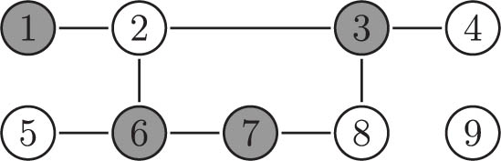
Network on nine units where the node label represents the number of a unit. Gray nodes receive the treatment, corresponding to
Example 1
Consider the network in Figure 1, where gray nodes take the treatment and white ones do not. We choose
2.2 Treatment effect and identification
Plugging in the outcome equation of the SEM (1), we can rewrite the treatment effect of interest, the EATE, as
where we obtain that the unit-specific treatment effect of unit
Estimating
Lemma 2.1
Let
be the concatenation of the observed variables for unit
including the aforementioned correction term. For the true nuisance functions
The aforementioned expectation is with respect to the law of
The proof of Lemma 2.1 is provided in Appendix E. Based on this lemma, we will present our estimator of
Scharfstein et al. [30] and Bang and Robins [31] considered a similar score
where
2.3 Dependency graph
Depending on the feature functions that are used, if an edge connects two units in the network
Definition 1
Dependency graph on
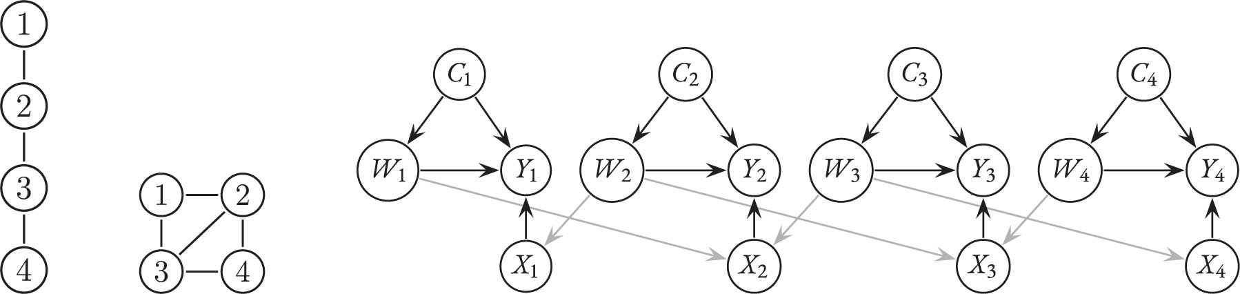
Network
Example 2
Consider the chain-shaped network
The dependency graph is a function of the network
2.4 Estimation procedure and asymptotics
Subsequently, we describe our estimation procedure and its asymptotic properties. We use sample splitting and cross-fitting to estimate the EATE
where
that averages over all
The partition
This aggregation scheme yields a valid overall p-value for the same two-sided test [38]. The corresponding confidence interval is constructed as
where typically
Next, we describe how
where
which can be solved for feasible values of
| Algorithm 1: Estimating the EATE from observational data on networks with spillover effects using plugin machine learning | |
|---|---|
|
Input:
|
|
|
Output: Estimator of the EATE
|
|
| 1 |
for
|
|
|
|
| 8 9 | end |
| 10 | Compute
|
| 11 | Compute aggregated p-value
|
| 12 | Compute confidence interval according to (8), call it
|
| 13 | Return
|
Before we present our main theorem we mentioned in the construction of confidence intervals earlier, we present and discuss key assumptions. First, we require that products of machine learning errors decay fast enough, namely,
(see Assumption A4 in the appendix for more details). In particular, the individual error terms may vanish at a rate smaller than
Assumption 1
The maximal degree
Ogburn et al. [6] only required
Furthermore, we require that this dependency structure is not too strong moment-wise in the sense that the variance term given in the following assumption converges.
Assumption 2
Let
where
Assuming bounded second moments,
where
Theorem 2.2
(Asymptotic distribution of
where
Please see Section E in the appendix for a proof of Theorem 2.2. The asymptotic variance
Our estimator
2.5 Bootstrap variance estimator
We use the residual bootstrap as follows to estimate the asymptotic variance. First, we use the estimated nuisance functions to compute the outcome regression residuals. More precisely, for
Theorem 2.3
The bootstrap scheme described in Section 2.5 consistently estimates the asymptotic variance (9) under Assumption A7 stated in the Appendix.
The proof of Theorem 2.3 can be found in Appendix F.
3 Empirical validation
We demonstrate our method in a simulation study and on a real-world dataset. In the simulation study, we validate the performance of our method on different network structures and compare it to two popular treatment effect estimators. Then, we investigate the effect of study time on exam performance in the Swiss StudentLife Study [27,28] taking into account the effect of social ties.
3.1 Simulation study
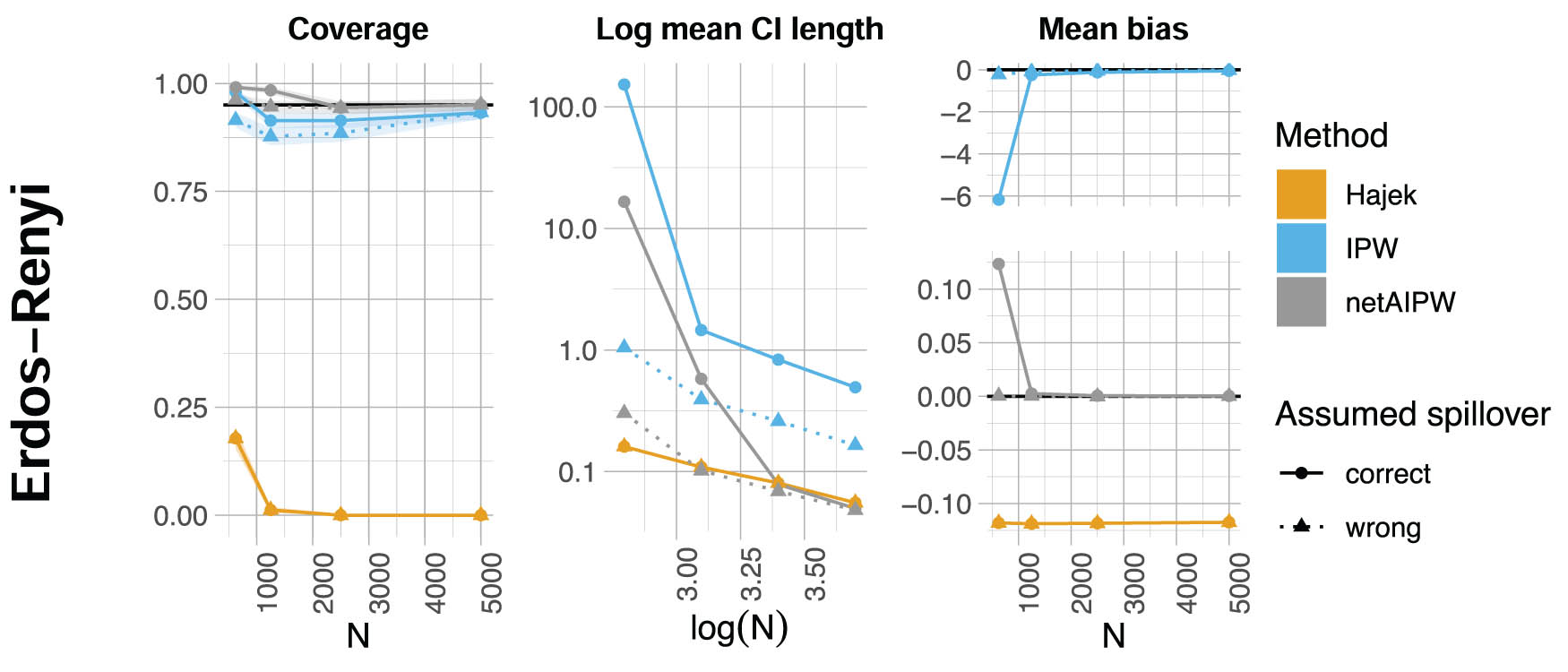
We investigate a fairly simple data-generating mechanism with 1-dimensional
We first describe the two competitors and then detail the simulation setting and present the results. Our code is available on GitHub (https://github.com/corinne-rahel/networkAIPW).
The Hájek estimator (denoted by “Hajek” in Figure 4) without incorporation of confounders [51] equals
The parametric convergence rate and asymptotic Gaussian distribution are preserved under
where
![Figure 3
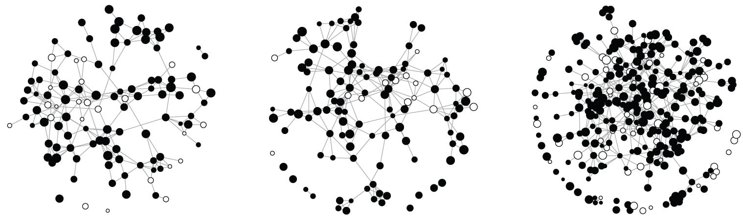
Different network structures on
N
=
200
N=200
units: Erdős–Rényi network (left) where two nodes are connected with probability
3
⁄
N
3/N
(every node is connected to three other nodes in expectation); Watts–Strogatz network (right) with a rewiring probability of 0.05, a 1-dimensional ring-shaped starting lattice where each node is connected to two neighbors on both sides (i.e., every node is connected to four other nodes), no loops, and no multiple edges. The graphs are generated using the R-package igraph [55].](/document/doi/10.1515/jci-2023-0082/asset/graphic/j_jci-2023-0082_fig_003.jpg)
Different network structures on
We investigate two network structures that govern our interference effects: Erdős–Rényi networks [56] and Watts–Strogatz networks [57]. Erdős–Rényi networks randomly form edges between units with a fixed probability and are a simple example of a random mathematical network model. These networks play an important role as a standard against which to compare more complicated models. Watts–Strogatz networks, also called small-world networks, share two properties with many networks in the real world: a small average shortest path length and a large clustering coefficient. To construct such a network, the vertices are first arranged in a regular fashion and linked to a fixed number of their neighbors. Then, some randomly chosen edges are rewired with a constant rewiring probability. A representative of each network type is provided in Figure 3. For each of these two network types, we consider one case where the dependency in the network does not increase with
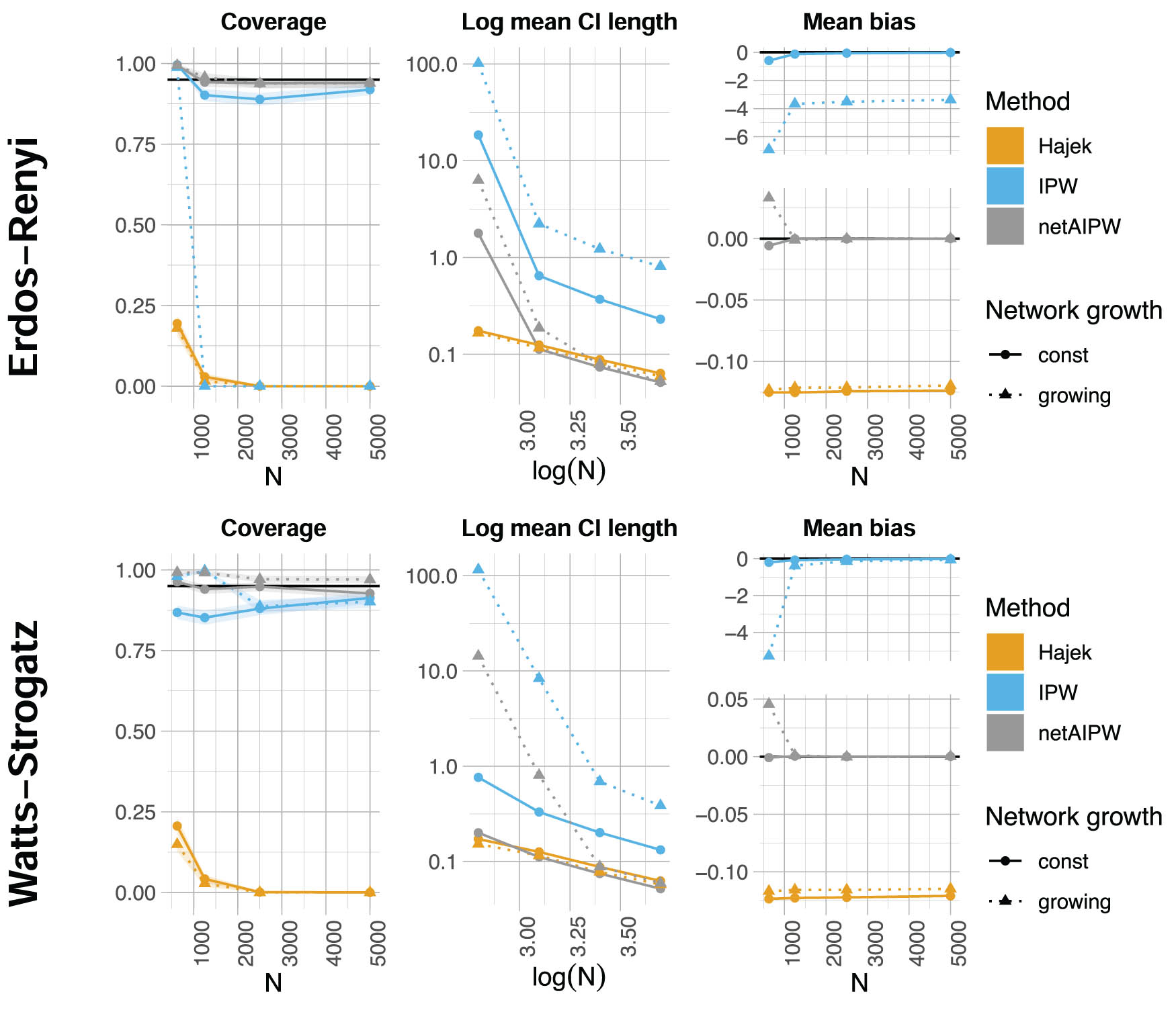
Coverage (fraction of times the true, and in general unknown,
The specific unit-level structural equations (1) we consider are as follows. For each unit
if
and
i.e., the functions
For the sample sizes
Simulation results involving spillover effects from second-degree neighbors and misspecified spillover effects are presented in Appendix C. Furthermore, for a
3.2 Empirical analysis: Swiss StudentLife study data
Subsequently, we estimate the causal effect of study time on academic success of university students with our newly developed estimator. We quantify this causal effect by the EATE that is the average of the difference in expected GPA of the final exam had a student studied much versus little, allowing for potential spillover effects from the student’s friends on the student’s study time. Among the factors that determine academic success are person-specific traits, such as intelligence [59], willingness to work hard [60], and socioeconomic background [61]. The Swiss StudentLife Study data [27,28] were collected to investigate the impact of various factors on academic achievement. It consists of observations from freshmen undergraduate students pursuing a degree in the natural sciences at a Swiss university. Instead of a university entrance test, these students had to pass a demanding examination after 1 year of studying. At several time points throughout this year, the students were asked to fill out questionnaires about their student life, social network, and well-being. The data consist of three cohorts of students. Cohort 1 was observed in 2016 and cohorts 2 and 3 in 2017. Importantly, for all three cohorts, the data contain friendship information among the students. We build the corresponding undirected network by drawing an edge between two students if at least one of them mentioned the other one as being a friend. We believe that spillover effects arise due to students interacting in this network, and thus, we have to control for them when estimating the EATE described earlier. Figure 5 displays the resulting network consisting of the three cohorts.
Friendship networks per cohort with black dots representing
GPA (
We estimated the EATE with two different definitions for
EATE and 95% confidence intervals for
| Spillover | EATE | 95% CI for
|
|---|---|---|
| (a)
|
||
| Yes | 0.362 | [0.283, 0.442] |
| No | 0.451 | [0.364, 0.528] |
| (b)
|
||
| Yes | 0.078 |
|
| No | 0.163 |
|
4 Conclusion
Causal inference with observational data usually assumes independent units. However, having independent observations is often questionable, and so-called spillover effects among units are common in practice. Our aim was to develop point estimation and asymptotic inference for the expected average treatment effect (EATE) with observational data from a single (social) network. We would like to point out the hardness of this problem: we consider treatment effect estimation on data with increasing dependence among units, where the data-generating mechanism can be highly nonlinear and include confounders. We use an augmented inverse probability weighting (AIPW) principle and account for spillover effects that we capture by features, which are functions of the known network and the treatment and covariate vectors. There may be several features, and one feature may capture spillover effects from different units than another feature; these units might be direct neighbors to compute one feature and neighbors of neighbors to compute another feature. We consider the dependency graph to pose assumptions on these features in our asymptotic theory. Units may interact beyond their direct neighborhoods, interactions may become increasingly complex as the sample size increases, and we consider arbitrary networks. Using ideas of double machine learning [20], we develop a cross-fitting algorithm under interference that allows us to estimate the nuisance components of our model by arbitrary machine learning algorithms. Although we employ machine learning algorithms, our EATE estimator converges at the
In a simulation study, we demonstrated that commonly employed methods for treatment effect estimation suffer from the presence of spillover effects, whereas our method could account for the complex dependence structures in the data so that the bias vanished with increasing sample size and coverage was guaranteed. In the Swiss StudentLife Study, we investigated the EATE of study time on the GPA of university examinations, accounting for spillover effects due to friendship relations. Omitting this spillover may lead to biased results due to spurious association.
In this work, we focused on estimating the EATE. Other effects may be estimated in a similar manner, for instance, the global average treatment effect (GATE) where all units are jointly intervened on. We develop an estimator of the GATE in Appendix H.
Acknowledgements
We thank the associate editor and reviewers for detailed and constructive comments. We also thank Leonard Henckel and Dominik Rothenhäusler for useful comments.
-
Funding information: CE and PB received funding from the European Research Council (ERC) under the European Union’s Horizon 2020 research and innovation programme (Grant Agreement No. 786461), and M-LS received funding from the Swiss National Science Foundation (SNF) (Project No. 200021_172485). The Swiss StudentLife data collection was supported by Swiss National Science Foundation Grant 10001A 169965 and the rectorate of ETH Zurich.
-
Author contributions: All authors have accepted responsibility for the en4re content of this manuscript and approved its submission.
-
Conflict of interest: The authors state no conflict of interest.
-
Data availability statement: The data and code used in the simula4on study are available on GitHub (https://github.com/corinne-rahel/networkAIPW). The Swiss StudentLife data analyzed in the empirical analysis is cited in the main text of our paper.
Appendix A A1 Assumptions and additional definitions
We consider the following notation. We denote by
We observe
Let the number of sample splits
Let
For completeness, we recall the following two assumptions from the main text. Assumption A1 limits the growth rate of the maximal degree of a node in the dependency graph. Assumption A2 characterizes the asymptotic variance in Theorem G.1 as the limit of the population variance on the
Assumption A1
The maximal degree
Assumption A2
Let
where
We make the following additional sets of assumptions. Assumption A3 recalls that we use the model (1) and specifies regularity assumptions on the involved random variables. Assumptions 3.2 and 3.3 ensure that the random variables are integrable enough. Assumption 3.4 ensures that the true underlying function
Assumption A3
Let
The structural equations (1) hold, where the treatment
There is a finite real constant
There is a finite real constant
There is a finite real constant
There is a finite real constant
Assumption A4 characterizes the realization set of the nuisance functions and the
Assumption A4
Consider the
The set
Assumption 3.4 also holds with
Let
i.e.,
For all
Assumption A5 and A6 are only required to establish that our plugin estimator of the asymptotic variance is consistent in Appendix G. (However, please recall that we recommend using the bootstrap procedure presented in Section 2.5 unless the sample size is large). They are not required to establish the asymptotic Gaussian distribution of our plugin machine learning estimator. Assumption A5 characterizes the order of the minimal size of the sets
Assumption A5
For
Assumption A6 specifies that all individual machine learning estimators of the nuisance functions converge at a rate faster than
Assumption A6
The slowest convergence rate
B Network effects in the social sciences
We consider models related to spillover effects. However, another notion of spillover effects has prevailed within the social science networks literature, namely, social influence effects. In this appendix, we describe social influence effects and how their modeling differs from our approach. Whereas spillover effects represent new covariates on the unit level that are built from variables of other units along network paths, social influence effects mostly concern effects that a specific variable
In contrast, the spillover features that we consider summarize variables from neighboring units. They represent a new variable that is used for the treatment or outcome regression models. For example, in our empirical analysis, we consider the spillover effect of study motivation of unit
C Additional simulation results
First, we present simulation results involving spillover effects from second-degree neighbors and misspecified spillover effects. We consider the same data-generating mechanism and estimation framework as in Section 3.1 apart from the following change: the “neighborhood”
Coverage (fraction of times the true, and in general unknown,
Next, we present networks and different kinds of spillover effects to show when Assumption A2 holds and when it fails to hold. We consider the same second-degree spillover effects and Erdős–Rényi network as mentioned earlier in this section. The “const” network has an expected degree of 2.5, and the “
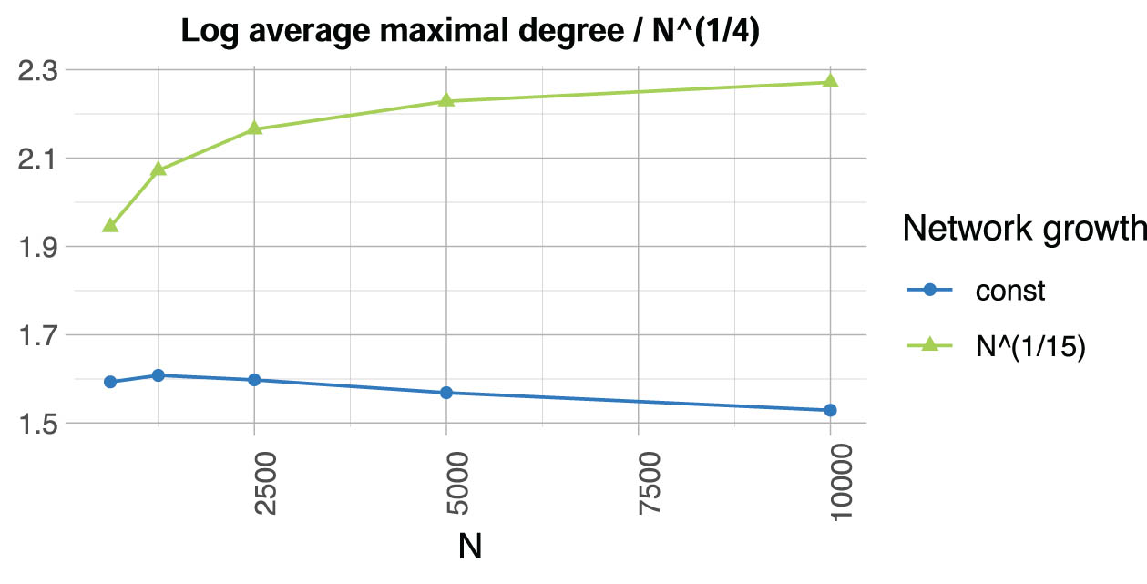
Simulated maximal degree of the dependency graph from second-degree spillover on Erdős–Rényi networks with an expected degree of either 2.5 (“const”) or
D Supplementary lemmata
In this section, we prove two results on conditional independence relationships of the variables from our model. We argue for the DAG of our model (1) and use graphical criteria [33–37,72,73]. We denote the direct causes of
Lemma D.1
Let
Proof of Lemma D.1
The parents of
Lemma D.2
Let
Proof of Lemma D.2
The parents of
E Proof of Theorem 2.2
Proof of Lemma 2.1
Let
We have
due to Lemma D.1 and because
The following lemma shows that the score function
Lemma E.1
(Neyman orthogonality) Assume that the assumptions of
Theorem 2.2
hold. Let
Proof of Lemma E.1
Let
We evaluate this expression at
due to (A2) and because
holds due to Lemma D.2 and because we assumed
The following lemma bounds the second directional derivative of the score function. Its proof uses that products of the errors of the machine learners are of a smaller order than
Lemma E.2
(Product property) Assume the assumptions of
Theorem 2.2
hold. Let
Proof of Lemma E.2
We use the first directional derivative we derived in (A3) to compute the second directional derivative
Due to Hölder’s inequality and Assumptions 3.1, 3.3, 3.4, and 4.1, we have
Due to Assumption 4.1, both summands mentioned earlier are bounded by
The following lemma describes how we apply Stein’s method [74] to obtain the asymptotic Gaussian distribution of our estimator although the data are highly dependent.
Lemma E.3
(Asymptotic distribution with Stein’s method) Assume the assumptions of Theorem 2.2 hold. Denote by
Observe that by
Assumption A2, we have
Proof of Lemma E.3
According to Lemma 2.1, we have
By assumption, we have
Lemma E.4
(Vanishing covariance due to sparse dependency graph) Assume the assumptions of
Theorem 2.2
hold. Let
Proof of Lemma E.4
Let
Let
Assumptions 3.1, 3.3, 3.4, and 4.2 bound the terms
with
Subsequently, we bound the summands in (A5). Due to (A6), we have
with
where
can be bounded by
where the last bound holds due to Assumption 4.3. Consequently, we have
with
Lemma E.5
(Taylor expansion) Assume the assumptions of
Theorem 2.2
hold. Let
Proof of Lemma E.5
Let
We have
We apply a Taylor expansion to
for some
Due to the definition of
with
Proof of Theorem 2.2
We have
because the disjoint sets
due to Hölder’s inequality and Lemmas E.4 and E.5. Because
Due to Lemma E.3, we have
as
F Bootstrap variance estimator
We use the following assumption to establish the consistency of the bootstrap variance estimator. It is a high-level assumption, and we will not verify it in terms of the model (1); yet, assuming some form of continuity (as below) seems to be essentially necessary for the bootstrap to be consistent.
Assumption A7
To make the dependence of
which can be represented as
due to
We assume that
Proof of Theorem 2.3
The bootstrap variance relies on the same dependency structure induced by the network as
where the construction of
Due to Assumption 3.1 and [76], we have
which consequently establishes consistency of the bootstrap variance.□
G Consistent plugin variance estimator
An alternative to the bootstrap variance estimator can be constructed as described below. We do not recommend this estimator unless the sample size is large relative to the network connectivity, but its consistency can be derived under different and more explicit conditions than in (A7).
The challenge is that the unit-level effects
We partition
where
Subsequently, we characterize a situation in which the index
Theorem G.1
Denote by
is a consistent estimator of the asymptotic variance
G.1 Proof of Theorem G.1
Lemma G.2
Assume the assumptions of
Theorem G.1
hold. Let
Proof of Lemma G.2
We have
All individual summands in the aforementioned decomposition are bounded by a finite real constant independent of
The other terms in the statement of the present lemma are bounded as well by finite real constants independent of
Moreover, we have
Furthermore, with
The term
Lemma G.3
(Convergence rate of unit-level effect estimators) Assume the assumptions of
Theorem G.1
hold. Let
Proof of Lemma G.3
Let
Subsequently, we show that the two sets of summands in (A9) are of order
due to equation (A6). Hence, we have
because we have
because
Consequently, we also have
Lemma G.4
(Consistent variance estimator part I) Assume the assumptions of Theorem G.1 hold. We have
Proof of Lemma G.4
We have
We bound the three sets of summands in (A10) individually. The first set of summands can be expressed as
We have
because the function
with
due to Hölder’s inequality. Hence, the first set of summands in (A10) is of order
We have
Consequently, the second set of summands in (A10) is of order
because
Lemma G.5
(Consistent variance estimator part II) Assume the assumptions of
Theorem G.1
hold. Denote by
Proof of Lemma G.5
We have the decomposition
Subsequently, we bound the three sets of summands in (A12) individually. We start by bounding the first set of summands. We have
We have
due to Hölder’s inequality, Lemma G.3, Lemma G.2, and Assumption A1. Moreover, we have
due to Hölder’s inequality, Lemma G.3, and Assumption A1. Consequently, the first set of summands in (A12) is of order
with
Due to Lemma G.2, the variance and covariance terms in (A13) are uniformly bounded by constants. Furthermore, the covariance terms do only not equal 0 if
due to Assumption A1. Therefore, we have established the statement of the present lemma because we have verified that all three sets of summands in (A12) are of order
Proof of Theorem G.1
The proof follows from Lemmas G.4 and G.5.□
H Extension to estimate global effects
So far, we focused on the EATE. We intervened on each individual unit and left the treatment selections of the other units as they were.
Subsequently, we consider another type of treatment effect where we assess the effect of a single intervention that intervenes on all subjects simultaneously. Instead of the EATE in (2), we subsequently consider the GATE with respect to the binary vector
where
We use the same definition for
In contrast to the score that we used for the EATE, this score includes additional factors
Let us denote by
the
denotes the feature vector where
denotes the feature vector where
where
To estimate
Theorem H.1
(Asymptotic distribution of
Then, the estimator
where
This theorem requires that the number of spillover effects a unit receives is bounded. Theorem 2.2 that establishes the parametric convergence rate and asymptotic Gaussian distribution of the EATE estimator did not require such an assumption. The reason is that
To estimate
Also van der Laan [14], Sofrygin and van der Laan [10], and Ogburn et al. [6] consider semiparametric estimation of the GATE using TMLE. They also require a uniform bound of the number of spillover effects a unit receives to achieve the parametric convergence rate of their estimator.
References
[1] Rubin D. Comment on: Randomization analysis of experimental data in the fisher randomization test by D. Basu. J Amer Stat Assoc. 1980;75:591–3. 10.2307/2287653Search in Google Scholar
[2] Perez-Heydrich C, Hudgens MG, Halloran E, Clemens JD, Ali M, Emch ME. Assessing effects of cholera vaccination in the presence of interference. Biometrics. 2014;70(3):731–41. 10.1111/biom.12184Search in Google Scholar PubMed PubMed Central
[3] Sävje F, Aronow PM, Hudgens MG. Average treatment effects in the presence of unknown interference. Ann Stat. 2021;49(2):673–701. 10.1214/20-AOS1973Search in Google Scholar
[4] Lee Y, Ogburn EL. Network dependence can lead to spurious associations and invalid inference. J Amer Stat Assoc. 2021;116(535):1060–74. 10.1080/01621459.2020.1782219Search in Google Scholar
[5] Sobel ME. What do randomized studies of housing mobility demonstrate? J Amer Stat Assoc. 2006;101(476):1398–407. 10.1198/016214506000000636Search in Google Scholar
[6] Ogburn EL, Sofrygin O, Diiiaz I, van der Laan MJ. Causal inference for social network data. J Amer Stat Assoc. 2022;0(0):1–15. Search in Google Scholar
[7] Eckles D, Bakshy E. Bias and high-dimensional adjustment in observational studies of peer effects. J Amer Stat Assoc. 2021;116(534):507–17. 10.1080/01621459.2020.1796393Search in Google Scholar
[8] Ogburn EL, VanderWeele TJ. Vaccines, contagion, and social networks. Ann Appl Stat. 2017;11(2):919–48. 10.1214/17-AOAS1023Search in Google Scholar
[9] Hudgens MG, Halloran E. Toward causal inference with interference. J Amer Stat Assoc. 2008;103(482):832–42. 10.1198/016214508000000292Search in Google Scholar PubMed PubMed Central
[10] Sofrygin O, van der Laan MJ. Semi-parametric estimation and inference for the mean outcome of the single time-point intervention in a causally connected population. J Causal Inference. 2017;5(1):1–35. 10.1515/jci-2016-0003Search in Google Scholar PubMed PubMed Central
[11] Pearl J. Causal diagrams for empirical research. Biometrika. 1995;82(4):669–88. 10.1093/biomet/82.4.669Search in Google Scholar
[12] Splawa-Neyman J, Dabrowska DM, Speed TP. On the application of probability theory to agricultural experiments. Essay on Principles. Section 9. Stat Sci. 1990;5(4):465–72. 10.1214/ss/1177012031Search in Google Scholar
[13] Rubin DB. Estimating causal effects of treatments in randomized and nonrandomized studies. J Educat Psychol. 1974;66(5):688–701. 10.1037/h0037350Search in Google Scholar
[14] van der Laan M. Causal inference for a population of causally connected units. J Causal Inference. 2014;2(1):13–74. 10.1515/jci-2013-0002Search in Google Scholar PubMed PubMed Central
[15] Manski CF. Identification of endogenous social effects: the reflection problem. Rev Econ Stud. 1993;60(3):531–42. 10.2307/2298123Search in Google Scholar
[16] Chin A. Regression adjustments for estimating the global treatment effect in experiments with interference. J Causal Inference. 2019;7(2):20180026. 10.1515/jci-2018-0026Search in Google Scholar
[17] Cai J, De Janvry A, Sadoulet E. Social networks and the decision to insure. Amer Econ J Appl Econ. 2015;7(2):81–108. 10.1257/app.20130442Search in Google Scholar
[18] Leung M. Treatment and spillover effects under network interference. Rev Econ Stat. 2020;102(2):368–80. 10.1162/rest_a_00818Search in Google Scholar
[19] Robins JM, Rotnitzky A, Zhao LP. Analysis of semiparametric regression models for repeated outcomes in the presence of missing data. J Amer Stat Assoc. 1995;90(429):106–21. 10.1080/01621459.1995.10476493Search in Google Scholar
[20] Chernozhukov V, Chetverikov D, Demirer M, Duflo E, Hansen C, Newey W, et al. Double/debiased machine learning for treatment and structural parameters. Econom J. 2018;21(1):C1–68. 10.1111/ectj.12097Search in Google Scholar
[21] Tchetgen Tchetgen EJ, Fulcher IR, Shpitser I. Auto-G-computation of causal effects on a network. J Amer Stat Assoc. 2021;116(534):833–44. 10.1080/01621459.2020.1811098Search in Google Scholar PubMed PubMed Central
[22] Robins J. A new approach to causal inference in mortality studies with a sustained exposure period-application to control of the healthy worker survivor effect. Math Model. 1986;7(9):1393–512. 10.1016/0270-0255(86)90088-6Search in Google Scholar
[23] Lauritzen SL, Richardson TS. Chain graph models and their causal interpretations. J R Stat Soc Ser B (Stat Methodol). 2002;64(3):321–48. 10.1111/1467-9868.00340Search in Google Scholar
[24] van der Laan MJ, Rubin D. Targeted maximum likelihood learning. Int J Biostat. 2006;2(1). 10.2202/1557-4679.1043Search in Google Scholar
[25] van der Laan MJ, Rose S. Targeted learning. Springer Series in Statistics. New York: Springer; 2011. 10.1007/978-1-4419-9782-1Search in Google Scholar
[26] van der Laan MJ, Rose S. Targeted learning in data science. Springer Series in Statistics. New York: Springer; 2018. 10.1007/978-3-319-65304-4Search in Google Scholar
[27] Stadtfeld C, Vörös A, Elmer T, Boda Z, Raabe IJ. Integration in emerging social networks explains academic failure and success. Proc Nat Acad Sci. 2019;116(3):792–7. 10.1073/pnas.1811388115Search in Google Scholar PubMed PubMed Central
[28] Vörös A, Boda Z, Elmer T, Hoffman M, Mepham K, Raabe IJ, et al. The Swiss StudentLife Study: Investigating the emergence of an undergraduate community through dynamic, multidimensional social network data. Soc Netw. 2021;65:71–84. 10.1016/j.socnet.2020.11.006Search in Google Scholar
[29] Bühlmann P. Sieve bootstrap for time series. Bernoulli. 1997;3(2):123–48. 10.2307/3318584Search in Google Scholar
[30] Scharfstein DO, Rotnitzky A, Robins JM. Adjusting for nonignorable drop-out using semiparametric nonresponse models. J Amer Stat Assoc. 1999;94(448):1096–120. 10.1080/01621459.1999.10473862Search in Google Scholar
[31] Bang H, Robins JM. Doubly robust estimation in missing data and causal inference models. Biometrics. 2005;61(4):962–72. 10.1111/j.1541-0420.2005.00377.xSearch in Google Scholar PubMed
[32] Robins JM, Rotnitzky A. Semiparametric efficiency in multivariate regression models with missing data. J Amer Stat Assoc. 1995;90(429):122–9. 10.1080/01621459.1995.10476494Search in Google Scholar
[33] Lauritzen SL. Graphical models. Oxford statistical science series. Oxford: Clarendon Press; 1996. 10.1093/oso/9780198522195.001.0001Search in Google Scholar
[34] Pearl J. Graphs, causality, and structural equation models. Sociol Meth Res. 1998;27(2):226–84. 10.1177/0049124198027002004Search in Google Scholar
[35] Pearl J. Causality: Models, reasoning, and inference. 2nd ed. Cambridge: Cambridge University Press; 2009. 10.1017/CBO9780511803161Search in Google Scholar
[36] Pearl J. An introduction to causal inference. Int J Biostat. 2010;6(2):7. 10.2202/1557-4679.1203Search in Google Scholar PubMed PubMed Central
[37] Perković E, Textor J, Kalisch M, Maathuis MH. Complete graphical characterization and construction of adjustment sets in markov equivalence classes of ancestral graphs. J Machine Learn Res. 2018;18(220):1–62. Search in Google Scholar
[38] Meinshausen N, Meier L, Bühlmann P. p-Values for high-dimensional regression. J Amer Stat Assoc. 2009;104(488):1671–81. 10.1198/jasa.2009.tm08647Search in Google Scholar
[39] Bickel PJ, Ritov Y, Tsybakov AB. Simultaneous analysis of lasso and dantzig selector. Ann Stat. 2009;37(4):1705–32. 10.1214/08-AOS620Search in Google Scholar
[40] Bühlmann P, van de Geer S. Statistics for high-dimensional data: methods, theory and applications. Springer Series in Statistics. Heidelberg: Springer; 2011. 10.1007/978-3-642-20192-9Search in Google Scholar
[41] Belloni A, Chernozhukov V, Wang L. Square-root lasso: pivotal recovery of sparse signals via conic programming. Biometrika. 2011;98(4):791–806. 10.1093/biomet/asr043Search in Google Scholar
[42] Belloni A, Chernozhukov V. Ell-penalized quantile regression in high-dimensional sparse models. Ann Stat. 2011;39(1):82–130. 10.1214/10-AOS827Search in Google Scholar
[43] Belloni A, Chen D, Chernozhukov V, Hansen C. Sparse models and methods for optimal instruments with an application to eminent domain. Econometrica. 2012;80(6):2369–429. 10.3982/ECTA9626Search in Google Scholar
[44] Belloni A, Chernozhukov V. Least squares after model selection in high-dimensional sparse models. Bernoulli. 2013;19(2):521–47. 10.3150/11-BEJ410Search in Google Scholar
[45] Kozbur D. Analysis of testing-based forward model selection. Econometrica. 2020;88(5):2147–73. 10.3982/ECTA16273Search in Google Scholar
[46] Luo Y, Spindler M. High-Dimensional L2 Boosting: Rate of Convergence; 2016. Preprint arXiv:1602.08927. Search in Google Scholar
[47] Wager S, Walther G. Adaptive Concentration of Regression Trees, with Application to Random Forests; 2016. Preprint arXiv:1503. 06388. Search in Google Scholar
[48] Chen X, White H. Improved rates and asymptotic normality for nonparametric neural network estimators. IEEE Trans Inform Theory. 1999;45:682–91. 10.1109/18.749011Search in Google Scholar
[49] Stein C. A bound for the error in the normal approximation to the distribution of a sum of dependent random variables. In: Proceedings of the sixth Berkeley symposium on mathematical statistics and probability, volume 2: Probability theory. vol. 6. University of California Press; 1972. p. 583–603. 10.1525/9780520423671-036Search in Google Scholar
[50] Smucler E, Rotnitzky A, Robins JM. A unifying approach for doubly-robust ell1 regularized estimation of causal contrasts; 2019. Preprint arXiv:1904.03737. Search in Google Scholar
[51] Hájek J. Comment on “An essay on the logical foundations of survey sampling, part one” by Basu. In: Godambe VP, Sprott DA, editors. Foundations of Statistical Inference. Toronto: Holt, Rinehart and Winston; 1971. p. 236. Search in Google Scholar
[52] Li S, Wager S. Random graph asymptotics for treatment effect estimation under network interference. Ann Stat. 2022;50(4):2334–58. 10.1214/22-AOS2191Search in Google Scholar
[53] Rosenbaum PR. Model-based direct adjustment. J Amer Stat Assoc. 1987;82(398):387–94. 10.1080/01621459.1987.10478441Search in Google Scholar
[54] Hirano K, Imbens G, Ridder G. Efficient estimation of average treatment effects using the estimated propensity score. Econometrica. 2003;71(4):1161–89. 10.1111/1468-0262.00442Search in Google Scholar
[55] Csardi G, Nepusz T. The igraph software package for complex network research. InterJournal. 2006;Complex Systems:1695. https://igraph.org. Search in Google Scholar
[56] Erdős P, Rényi A. On random graphs I. Publicationes Mathematicae. 1959;6:290–7. 10.5486/PMD.1959.6.3-4.12Search in Google Scholar
[57] Watts DJ, Strogatz S. Collective dynamics of ‘small-world’ networks. Nature. 1998;393:440–2. 10.1038/30918Search in Google Scholar PubMed
[58] Wright MN, Ziegler A.A fast implementation of random forests for high dimensional data in C++ and R. J Stat Softw. 2017;77(1):1–17. 10.18637/jss.v077.i01Search in Google Scholar
[59] Chamorro-Premuzic T, Furnham A. Personality, intelligence and approaches to learning as predictors of academic performance. Personality Individual Differ. 2008;44(7):1596–603. 10.1016/j.paid.2008.01.003Search in Google Scholar
[60] Los R, Schweinle A. The interaction between student motivation and the instructional environment on academic outcome: a hierarchical linear model. Soc Psychol Educat. 2019;22(2):471–500. 10.1007/s11218-019-09487-5Search in Google Scholar
[61] Heckman JJ. Skill formation and the economics of investing in disadvantaged children. Science. 2006;312(5782):1900–2. 10.1126/science.1128898Search in Google Scholar PubMed
[62] Spinath B, Stiensmeier-Pelster J, Schoene C, Dickhäuser O. Skalen zur Erfassung der Lern- und Leistungsmotivation: SELLMO. Bern: Hogrefe Verlag; 2002. Search in Google Scholar
[63] Cohen S, Williamson G. Perceived stress in a probability sample of the United States. In: Spacapam S, Oskamp S, editors. The Social Psychology of Health: Claremont Symposium on Applied Social Psychology. Newbury Park, CA: Sage; 1988. Search in Google Scholar
[64] Lattimore T, Szepesvári C. Bandit algorithms. Cambridge: Cambridge University Press; 2020. 10.1017/9781108571401Search in Google Scholar
[65] Ugander J, Karrer B, Backstrom L, Kleinberg J. Graph cluster randomization: network exposure to multiple universes; 2013. Preprint arXiv:1305. 6979. 10.1145/2487575.2487695Search in Google Scholar
[66] Eckles D, Karrer B, Ugander J. Design and analysis of experiments in networks: reducing bias from interference. J Causal Infer. 2017;5(1):20150021. 10.1515/jci-2015-0021Search in Google Scholar
[67] Robins G, Pattison P, Elliott P. Network models for social influence processes. Psychometrika. 2001;66(2):161–89. 10.1007/BF02294834Search in Google Scholar
[68] Daraganova G, Robins G. Autologistic actor attribute models. In: Lusher D, Koskinen J, Robins G, editors. Structural analysis in the social sciences. Cambridge: Cambridge University Press; 2012. p. 102–14. 10.1017/CBO9780511894701.011Search in Google Scholar
[69] Snijders TAB. Models for longitudinal network data. In: Carrington PJ, Scott J, Wasserman S, editors. Structural Analysis in the Social Sciences. Cambridge: Cambridge University Press; 2005. p. 215–47. 10.1017/CBO9780511811395.011Search in Google Scholar
[70] Snijders TAB, van de Bunt GG, Steglich CEG. Introduction to stochastic actor-based models for network dynamics. Soc Netw. 2010;32(1):44–60. 10.1016/j.socnet.2009.02.004Search in Google Scholar
[71] Steglich C, Snijders TAB, Pearson M. Dynamic networks and behavior: separating selection from influence. Sociol Methodol. 2010;40(1):329–93. 10.1111/j.1467-9531.2010.01225.xSearch in Google Scholar
[72] Peters J, Janzing D, Schölkopf B. Elements of causal inference: Foundations and learning algorithms. Adaptive Comput Machine Learn. Cambridge, MA: The MIT Press; 2017. Search in Google Scholar
[73] Maathuis M, Drton M, Lauritzen S, Wainwright M, editors. Handbook of graphical models. Handbooks of Modern Statistical Methods. Boca Raton, FL: Chapman & Hall/CRC; 2019. 10.1201/9780429463976Search in Google Scholar
[74] Chin A. Central limit theorems via Stein’s method for randomized experiments under interference; 2018. Preprint arXiv:1804.03105. Search in Google Scholar
[75] Ross N. Fundamentals of Stein’s method. Probability surveys. 2011;8(none):210–93. 10.1214/11-PS182Search in Google Scholar
[76] Bickel PJ, Freedman DA. Some asymptotic theory for the bootstrap. Ann Stat. 1981;9(6):1196–217. 10.1214/aos/1176345637Search in Google Scholar
© 2025 the author(s), published by De Gruyter
This work is licensed under the Creative Commons Attribution 4.0 International License.
Articles in the same Issue
- Research Articles
- Decision making, symmetry and structure: Justifying causal interventions
- Targeted maximum likelihood based estimation for longitudinal mediation analysis
- Optimal precision of coarse structural nested mean models to estimate the effect of initiating ART in early and acute HIV infection
- Targeting mediating mechanisms of social disparities with an interventional effects framework, applied to the gender pay gap in Western Germany
- Role of placebo samples in observational studies
- Combining observational and experimental data for causal inference considering data privacy
- Recovery and inference of causal effects with sequential adjustment for confounding and attrition
- Conservative inference for counterfactuals
- Treatment effect estimation with observational network data using machine learning
- Causal structure learning in directed, possibly cyclic, graphical models
- Mediated probabilities of causation
- Beyond conditional averages: Estimating the individual causal effect distribution
- Matching estimators of causal effects in clustered observational studies
- Ancestor regression in structural vector autoregressive models
- Single proxy synthetic control
- Bounds on the fixed effects estimand in the presence of heterogeneous assignment propensities
- Minimax rates and adaptivity in combining experimental and observational data
- Highly adaptive Lasso for estimation of heterogeneous treatment effects and treatment recommendation
- A clarification on the links between potential outcomes and do-interventions
- Valid causal inference with unobserved confounding in high-dimensional settings
- Spillover detection for donor selection in synthetic control models
- Causal additive models with smooth backfitting
- Experiment-selector cross-validated targeted maximum likelihood estimator for hybrid RCT-external data studies
- Applying the Causal Roadmap to longitudinal national registry data in Denmark: A case study of second-line diabetes medication and dementia
- Orthogonal prediction of counterfactual outcomes
- Variable importance for causal forests: breaking down the heterogeneity of treatment effects
- Multivariate zero-inflated causal model for regional mobility restriction effects on consumer spending
- Rate doubly robust estimation for weighted average treatment effects
- Adding covariates to bounds: what is the question?
- Review Article
- The necessity of construct and external validity for deductive causal inference