Regression(s) discontinuity: Using bootstrap aggregation to yield estimates of RD treatment effects
-
Mark C. Long
 and
Jordan Rooklyn
and
Jordan Rooklyn

Abstract
Following Efron (2014), we propose an algorithm for estimating treatment effects for use by researchers employing a regression-discontinuity (RD) design. This algorithm generates a set of estimates of the treatment effect from bootstrapped samples, wherein the polynomial-selection algorithm developed by Pei, Lee, Card, and Weber (2021) is applied to each sample, the average of these RD treatment effect (RDTE) estimates is computed and serves as the overall estimate of the RDTE. Effectively, this procedure estimates a set of plausible RD estimates and weights the estimates by their likelihood of being the best estimate to form a weighted-average estimate. We discuss why this procedure may lower the estimate’s root mean squared error (RMSE). In simulation results, we show that this better performance is achieved, yielding up to a 5% reduction in RMSE relative to PLCW’s method and a 16% reduction in RMSE relative to Calonico, Cattaneo, and Titiunik’s (2014) method for bandwidth selection (with default settings).
1 Introduction
This article applies the insights of Efron [1] and builds on the methods of Imbens and Kalyanaraman (IK, [2]), Calonico, Cattaneo, and Titiunik (CCT, [3]), and Pei, Lee, Card, and Weber (PLCW, [4]), each of which develop data-driven methods for estimating treatment effects in the context of a regression-discontinuity (RD) design. The RD design for estimating treatment effects was first used by Thistlethwaite and Campbell [5]. Hahn et al. evaluate the conditions that are necessary to identify the treatment effect in an RD design [6]. Cattaneo and Titiunik [7] provide a review of contemporary methods for estimating treatment effects in RD designs and an earlier review can be found in the study by Imbens and Lemieux [8]. Cattaneo et al. [9,10] provide “an accessible and practical guide for the analysis and interpretation of RD designs” (abstract). We review the IK, CCT, and PLCW methods to foreground our proposed approach (which we label as “LR”).
IK derive an optimal bandwidth assuming that the user is employing a local linear regression estimator. IK define this optimal bandwidth as “the bandwidth that minimizes a first-order approximation to MSE(
Note that this optimal bandwidth contains a series of estimated components. As such, the optimal bandwidth is not known with certainty. Perhaps in response, software by Nichols [11] to implement the IK bandwidth presents the user with estimates of the RDTE using the estimated IK bandwidth and this bandwidth doubled and it cut in half. This lack of certainty about the optimal bandwidth plays a key role in motivating our proposed approach.
CCT [3] build on the IK method in several respects. They develop robust confidence interval estimators for average treatment effects that are centered around a bias-corrected RD estimator. The “bias” in the conventional RD estimate arises as, for any given polynomial order choice (e.g., linear), there may be remaining higher-order curvature that causes the point estimate to be biased. Note that the IK bandwidth in equation (1) trades off an increase in bias that results from a larger bandwidth with the concurrent decrease in variance achieved by widening the bandwidth. Such optimal bandwidth algorithms produce bandwidths that are “too wide” in the sense that they permit bias to creep into the RDTE estimate. CCT generate a bias-corrected RDTE estimate that adjusts the conventional RDTE estimate with an estimate of the bias. They estimate the unknown derivatives in the leading bias term by using a higher-order local polynomial in order to construct this estimate of the bias [12]. CCT’s confidence intervals are “robust” as they add to the estimated conventional variance the variance that comes from having to estimate the leading bias. This additional source of variance “could be interpreted as the contribution of the bias correction to the variability of the bias-corrected estimator” (CCT, 2014b, p. 921). Their robust bias-corrected confidence intervals are as follows (CCT, 2014b, p. 914):
where
CCT [3] conduct simulations using three data-generating processes (DGPs). Assuming a linear polynomial specification, they show that using the IK optimal bandwidth to generate conventional RDTE estimates with conventional standard errors yields confidence interval coverage rates that are too low. The 95% confidence interval around the estimated RDTE contained the true RDTE in only 82.3, 30.3, and 84.2% of cases for these three DGPs, respectively (CCT [3], third column of Table 1, pp. 2316–7). In contrast, the 95% confidence intervals around the bias-corrected estimated RDTEs with bias-corrected variance contained the true RDTE in 91.6, 93.2, and 93.3% of cases for these three DGPs (CCT [3], ninth column of Table 1, pp. 2316–7), much closer to the expected 95% rate. Although these coverage rates are a clear improvement, it should be noted that they are still modestly below the 95% target. While these robust confidence intervals add variance to account for the estimation of the bias correction, they do not account for uncertainty in the width of the bandwidth. In contrast, our approach does account for this uncertainty and thus is more able to produce coverage rates close to 95%.[1]
Example illustrating our approach
| Method | Polynomial order | Frequency | Minimum bandwidth | Bandwidth | Maximum bandwidth | Standard deviation of bandwidth | Effective number of observations on the left (right) of cutoff | Conventional estimated RDTE | Standard error of the conventional estimated RDTE | 95% Confidence interval |
|---|---|---|---|---|---|---|---|---|---|---|
| CCT | 1 (Default) | — | — | 0.153 | — | — | 62 (37) | 0.081 | 0.055 | [‒0.028, 0.190] |
| PLCW | 0 (Selected) | — | — | 0.068 | — | — | 26 (21) | 0.107 | 0.039 | [0.028, 0.186] |
| LR | 0 | 151 | 0.039 | 0.065 | 0.110 | 0.013 | — | 0.105 | 0.044 | — |
| 1 | 45 | 0.089 | 0.174 | 0.270 | 0.042 | — | 0.074 | 0.047 | — | |
| 2 | 4 | 0.190 | 0.211 | 0.230 | 0.018 | — | 0.029 | 0.076 | — | |
| 3 | 0 | — | — | — | — | — | — | — | — | |
| 4 | 0 | — | — | — | — | — | — | — | — | |
| Overall | 200 | 0.039 | 0.092 | 0.270 | 0.054 | 35.9 (25.0) | 0.095 | 0.050 | [‒0.004, 0.186] |
Notes: The full sample consists of 500 observations with 406 (94) to the left (right) of the treatment cutoff. “Bandwidth” is the bandwidth used to identify the estimate of the RDTE (as opposed to the bandwidth used to estimate the bias). For our approach (LR), the “Bandwidth,” “Effective Number…,” and “Conventional Estimated RDTE” columns show the average values across bootstrapped samples. A uniform kernel weight is used for all three methods.
Using a local linear regression applied to data within either the IK or CCT bandwidths is the dominant method used in RD studies at this time.[2] Yet, it is also still popular for scholars to use higher-order polynomials applied to the whole span of the observed data. There are strong arguments against this approach. While higher-order polynomials may have a stronger fit to the whole of the data on a given side of the threshold, their out-of-sample predictive power may be weak and standard errors on their estimated RDTEs may be quite large. Gelman and Imbens [17] note that “we do not have good methods for choosing that order in a way that is optimal for the objective of a good estimator for the causal effect of interest” and “optimizing some global goodness-of-fit measure … is not closely related to the research objective of causal inference” (p. 447).
This backdrop sets the stage for PLCW’s method for selecting the optimal polynomial order. PLCW’s method is to compare the estimated asymptotic mean squared error for a variety of polynomial orders, with the optimal bandwidth for each polynomial chosen using CCT’s method, and select the order that minimizes this estimated AMSE. In simulations that test and compare polynomials of order 0 (i.e., a kernel-weighted average) to order 4 (i.e., a kernel-weighted quartic regression), PLCW show that using this polynomial-order-selection method can produce lower mean squared errors than the common default approach of using a local linear regression. Furthermore, they show that for a given DGP, there may exist a threshold sample size above which the optimal polynomial switches from lower order (e.g., linear) to higher order (e.g., quadratic).
We believe that the PLCW approach (which wraps around the CCT approach) is attractive and likely to be widely used. However, this approach does raise questions. First, note that at the sample size threshold at which the optimal polynomial order switches from linear to quadratic, one should be agnostic about whether the RDTE estimate from the linear specification is better or worse than the RDTE estimate from the quadratic specification. If these two RDTE estimates differ from one another, then an average of these two RDTE estimates is likely to yield better performance (i.e., a lower mean squared error) than one obtains from either of these separate estimates taken by itself. Second, note that the PLCW method produces an estimate of the AMSE for each polynomial order and each order will generate a regression estimated using data within an estimated optimal bandwidth. Since the optimal bandwidth and resulting AMSE are not known with certainty, the optimal polynomial order cannot be known with certainty.
Efron [1] considers problems of this type. He notes that data-based model selection may yield “jumpy” estimates. Efron builds on the bootstrap aggregation (i.e., “bagging”) technique commonly used in machine learning to combine regression or classification trees [18]. Using this bootstrapped smoothing approach, which in the RD context would reduce the variability in the treatment effect estimation, Efron demonstrates how to compute appropriate standard errors and confidence intervals that take into account the model-selection procedure. This is a frequentist model averaging approach. Steel [19] notes that frequentist model averaging estimators can be described as weighted averages of parameters chosen from different models and notes that the key challenge is finding the appropriate weights. For further discussion of model averaging strategies and the additional uncertainty caused by model selection methods, see [20].
We follow Efron [1] by applying bootstrap aggregation to produce smoothed estimates of the treatment effect in RD contexts. Our approach, described in the next section, attempts to produce a weighted-average RDTE, which is composed of a set of RDTEs estimated using various polynomial orders and various bandwidths with each estimate weighted by the specification’s probability of yielding the lowest AMSE. In the third section, we provide an example to illustrate the method and simulation evidence. Across five DGPs, we show that our approach yields lower mean squared errors and better coverage rates than (a) CCT’s [3] method applied using a local linear regression for both the conventional and bias-corrected RDTEs and (b) PLCW’s [4] method for polynomial order selection followed by CCT’s [3] method for bandwidth selection for a given polynomial order.
2 Our proposed approach
From the complete set of observations from sample size
This data-driven algorithm has desirable features. First, the process produces the frequencies by which each polynomial order is selected by PLCW’s method across the 200 bootstrapped samples. If there is little uncertainty about the optimal order, then the 200 bootstrapped samples will be likely to select the same polynomial order. In contrast, if there is uncertainty, the algorithm will effectively weight the various polynomial orders by their respective likelihood of being the “best” (i.e., having the lowest estimated AMSE). Second, uncertainty about the size of the optimal bandwidth will be captured by variation in the bandwidths across the 200 samples. If there is little uncertainty in the optimal bandwidth, then the widths will be close to the same across the 200 samples. Yet, as we show below, there is considerable uncertainty in both the optimal polynomial order and the optimal bandwidths for given orders for the DGPs we examine.
Regarding inference, we consider two approaches. The first approach estimates the standard error simply from the standard deviation of estimated RDTEs (call this “
The second approach comes from Efron [1], who shows that the first approach generates confidence intervals that are too wide. Efron produces a “smoothed interval…
While the second approach is superior, we use the first approach (i.e.,
Our approach is related to, but different from, a simple bootstrapping approach [24]. The typical use of bootstrapping is to construct a confidence interval around a sample statistic by conducting the same procedure (e.g., computation of a sample median and computation of parameters of a particular regression) on repeated random samples with replacement. In such bootstrapping applications, a confidence interval is drawn around the statistic that is estimated on the full sample. It is generally not advised to use the mean of the bootstrapped samples’ estimates of the statistic as one’s estimate of the population parameter as “the bootstrapped statistic is one further abstraction away from your population parameter” and is “an estimate of an estimate” (Dima) [25]. Each bootstrapped sample, by itself, produces an unbiased but less efficient estimate of the population parameter than can be obtained from the full sample statistic. Yet, this efficiency loss may be less than the efficiency gain that can be achieved by allowing for variation in the bandwidth and polynomial order across the bootstrapped samples. By allowing for this specification variation across samples, we are not, in fact, estimating the same sample parameters for each bootstrapped sample, and thus our approach differs from standard bootstrapping applications.
It thus becomes an empirical question whether our approach introduces net efficiency gains. In the simulation results we show below, the mean squared error, averaged across various DGPs and various sample sizes, is slightly smaller using our approach than PLCW’s method and substantially smaller than using an assumed linear specification with CCT’s [3] optimal bandwidth, suggesting efficiency gains can be had in using our approach. Furthermore, even in cases where our approach produces a higher mean squared error, the differences are usually small. That is, if there is an efficiency loss in a given setting, it appears likely to be small.
Finally, there is the question of what kernel weight to use in the regressions. Triangular kernels that place more weight on observations near to the threshold and with a steadily declining weight throughout the range of
Our approach can be implemented using our user-written Stata command rdwa.[7] For example, the user might enter “rdwa y x, c(0) p_min(0) p_max(4) rbc kernel(uni) samples(4000) efron2014”, where “y” is the outcome of interest, “x” is the forcing variable determining treatment status, “c(0)” sets the cutoff for treatment at
3 Example and simulation evidence
We test the efficacy of our approach using five DGPs:
L1:
LM1:
L2: Same as L1 except
LM2: Same as LM1 except
J1:
The first two DGPs have been used in the simulation evidence provided in IK [2], CCT [3] and PLCW [4], and are derived from fifth-order polynomials fit on data from, respectively, Lee [27] and Ludwig and Miller [28]. The third and fourth DGPs are identical to the first and second, except that they multiply the standard deviation of
We assume that all observations to the right of the threshold are treated. That is, we are considering a “sharp” RD design.[8]
To illustrate our approach, we begin by creating one sample with 500 observations drawn from the L1 DGP. Table 1 presents the results with the CCT and PLCW methods and our approach applied to this sample.
The first row shows the results using Calonico et al.’s (2018) rdrobust command with default settings, including the default setting of a linear polynomial, but with a uniform kernel. This method produces a conventional (non-bias-corrected) RDTE estimate of 0.081. Note that this RDTE is double the true RDTE of 0.04 for the L1 DGP. The confidence interval for this estimate [‒0.028 to 0.190] includes, (i.e., “covers”) the true RDTE of 0.04. In the second row, we show the results applying PLCW’s method to select the optimal bandwidth, assuming one uses CCT’s method with default rdrobust settings for each considered polynomial order. PLCW’s method concludes that using a zero-order polynomial (i.e., a kernel-weighted average) will yield the lowest AMSE. Using this order, which produces a smaller bandwidth than the linear polynomial, yields a conventional RDTE estimate of 0.107 and a confidence interval of [0.028 to 0.196]. This estimate again covers the true RDTE of 0.04, but is a little worse than the CCT result as the RDTE estimate is further from the true value (i.e.,
The bottom six rows of Table 1 show our approach. We find that the polynomial order 0 is selected in 151 of our 200 bootstrapped samples, order 1 is selected for 45 samples, order 2 is selected for 4 samples, and orders 3 and 4 are never selected. Thus, our approach suggests that roughly three-quarters of the weight should be placed on the zero-order polynomial specifications, and most of the rest of the weight should be placed on linear specifications. Furthermore, note that within each of the polynomial orders, we find substantial variation in the optimal bandwidth. For example, for the zero-order polynomials, we find a mean bandwidth of 0.065 (very similar to the bandwidth selected by the PLCW method, 0.068), yet this bandwidth varies across the 151 samples from a low of 0.039 to a high of 0.110. The “Conventional Estimated RDTE” column shows that the polynomial orders produce fairly different estimated RDTEs: 0.105 for order 0, 0.074 for order 1, and
Figures 1, 2, 3 provide greater clarity on the results using our approach. Figure 1 shows the scatterplot of the 500 observations drawn from the L1 DGP, regression lines drawn using PLCW’s preferred specification (purple and green), and 200 regression lines applying PLCW’s method to 200 bootstrapped samples (red and blue). This figure shows that the zero-order polynomial is the dominant choice, but there are a sizable contingent of linear regression lines included and a faint hint of quadratic specifications. Furthermore, this figure shows that bandwidths vary considerably and are larger for the higher-order specifications.

Example illustrating our approach: Specification choice and regression lines.

Example illustrating our approach: Histogram of the estimated RDTEs.

Example illustrating the our approach: Effective weights as a function of the kernel weight applied to each of 200 samples. (a) Uniform Kernels and (b) triangular kernels.
Figure 2 shows a histogram of the estimated RDTEs across the 200 samples. The overall estimate of the RDTE is given by the vertical maroon line at 0.095. Two 95% confidence intervals are illustrated. The long dashed lines give a “percentile-based” confidence interval suggested by the histogram itself, whereby there are five estimated RDTEs to the left and right of these long dashed lines and 190 estimated RDTEs (i.e., 95%) in between. The short dashed lines gives a “normal-based” confidence interval stemming from assuming that the RDTEs are distributed
Figure 3 shows the effective weight placed on observations as a function of the value of
Next, we show how these methods compare when applied repeatedly across samples drawn from the five DGPs using three sample sizes, 500, 5,000, and 50,000. These sample sizes were chosen as they are broadly representative of the RD literature. To assess this contention, we conducted two literature searches on scholar.google.com. First, we chose “Show top recommendations” and searched for “Regression Discontinuity.” We compiled the first 30 articles that were using RD methods to estimate a causal impact and excluded literature review articles or articles that principally developed RD methods. From these 30 articles, we identified the full sample size from the first RD estimate shown in a table in the article.[9] Most of these “top” articles were more than a decade old. We then repeated this search by choosing “Show all recommendations” and restricted the search to articles published “Since 2017.”[10] The median sample size was 2,917 for “top” articles and 3,005.5 for “recent” articles. Of these 60 articles, seven had sample sizes below 500 and eight had sample sizes above 50,000. Appendix Figure A2 shows the distribution of these sample sizes, and Appendix Table A1 gives details on the 60 studies.[11]
Table 2 shows the results for 500 draws from the L1 DGP. We present the root mean squared errors (RMSEs) and coverage rates for both the conventional and bias-corrected estimated RDTEs. Single check marks denote the specification that has the lowest RMSE or coverage rate closest to 0.95 within sample size and kernel across the three methods, and double check marks denote the best performance within sample size across the six method
Simulation results for the L1 DGP
| Conventional RDTE | Bias-corrected RDTE | |||||||||
|---|---|---|---|---|---|---|---|---|---|---|
| Sample size | Kernel | Method | RMSE | Coverage rate | RMSE | Coverage rate | ||||
| 500 | Triangular | CCT | 0.062 | ✓✓ | 0.910 | ✓ | 0.070 | 0.926 | ||
| PLCW | 0.067 | 0.730 | 0.061 | ✓✓ | 0.906 | |||||
| LR | 0.064 | 0.908 | 0.063 | 0.948 | ✓✓ | |||||
| Uniform | CCT | 0.062 | ✓ | 0.892 | 0.066 | 0.918 | ||||
| PLCW | 0.067 | 0.794 | 0.062 | ✓ | 0.908 | |||||
| LR | 0.062 | 0.918 | ✓✓ | 0.062 | 0.946 | ✓ | ||||
| 5,000 | Triangular | CCT | 0.027 | 0.750 | 0.025 | 0.866 | ||||
| PLCW | 0.027 | 0.752 | 0.025 | 0.858 | ||||||
| LR | 0.024 | ✓✓ | 0.892 | ✓✓ | 0.024 | ✓ | 0.898 | ✓ | ||
| Uniform | CCT | 0.029 | 0.712 | 0.026 | 0.848 | |||||
| PLCW | 0.029 | 0.714 | 0.025 | 0.876 | ||||||
| LR | 0.025 | ✓ | 0.888 | ✓ | 0.024 | ✓✓ | 0.920 | ✓✓ | ||
| 50,000 | Triangular | CCT | 0.011 | 0.818 | 0.009 | 0.920 | ||||
| PLCW | 0.009 | 0.872 | 0.009 | ✓✓ | 0.932 | |||||
| LR | 0.009 | ✓✓ | 0.934 | ✓ | 0.009 | 0.954 | ✓ | |||
| Uniform | CCT | 0.011 | 0.794 | 0.010 | 0.900 | |||||
| PLCW | 0.010 | 0.876 | 0.009 | 0.920 | ||||||
| LR | 0.009 | ✓ | 0.938 | ✓✓ | 0.009 | ✓ | 0.952 | ✓✓ | ||
| Results | Triangular | CCT | 0.033 | 0.826 | 0.035 | 0.904 | ||||
| above | PLCW | 0.034 | 0.785 | 0.032 | ✓ | 0.899 | ||||
| averaged | LR | 0.032 | ✓ | 0.911 | ✓ | 0.032 | 0.933 | ✓ | ||
| Uniform | CCT | 0.034 | 0.799 | 0.034 | 0.889 | |||||
| PLCW | 0.035 | 0.795 | 0.032 | 0.902 | ||||||
| LR | 0.032 | ✓✓ | 0.915 | ✓✓ | 0.031 | ✓✓ | 0.939 | ✓✓ | ||
| Relative | PLCW(ct)/CCT(ct) | 1.038 | PLCW(bt)/CCT(bt) | 0.908 | ||||||
| performance | LR(cu)/CCT(ct) | 0.978 | LR(bu)/CCT(bt) | 0.906 | ||||||
| LR(cu)/PLCW(ct) | 0.943 | LR(bu)/PLCW(bt) | 0.997 | |||||||
| LR(cu)/CCT(bt) | 0.929 | |||||||||
| LR(cu)/PLCW(bt) | 1.023 | |||||||||
Notes: The CCT rows show the results assuming a linear regression using CCT’s optimal bandwidth selection method applied to a linear specification. PLCW rows use PLCW’s method for polynomial order selection assuming CCT’s optimal bandwidth. LR rows use our approach of bootstrap aggregation of the PLCW method. The coverage rates are computed assuming conventional standard errors for the conventional RDTE estimates and robust standard errors for the bias-corrected results. Single check marks denote the specification that has the lowest RMSE or coverage rate closest to 0.95 within sample size and kernel across the three methods, and double check marks denote the best performance within sample size across the six
With a sample size of 500, the lowest RMSE is found for the CCT-triangular-kernel specification for the conventional RDTE (0.062) and the PLCW-triangular-kernel specification for the bias-corrected RDTE (0.061), yet these specifications provide coverage rates that are low (0.910 and 0.906, respectively). These RMSEs are narrowly better than that found using the LR-uniform specification (0.062 and 0.062, respectively), while LR-uniform yields better coverage rates (0.918 and 0.946, respectively).
In the next panel, we show the results for the 5,000 sample size. Our specification produces the lowest RMSE and best coverage rates for the conventional RDTE using a triangular kernel and for the bias-corrected RDTE using a uniform kernel. For sample size 50,000, the lowest RMSEs are 0.009, which are achieved by both the LR and PLCW specifications. Yet, our approach again produces better coverage rates for these estimates.
In the bottom panel of Table 2, we average the results from the three panels above. We find that our approach with a uniform kernel produces the best results across the board. For users preferring the conventional RDTE, our approach produces the lowest RMSE and best coverage rates. The same is true if the user prefers a bias-corrected RDTE estimate. The final five rows of Table 2 show the relative performance of these specifications. For this analysis, we assume that users of CCT’s and PLCW’s methods are prone to use triangular kernel weights and bias-corrected RDTE estimates. We find that PLCW’s method yields a 9% reduction in RMSE relative to CCT’s method when using bias-corrected RDTE estimates, thus replicating PLCW’s findings. In the subsequent rows, we compare CCT’s and PLCW’s methods to our approach. The bottom two rows show the comparisons assuming the user of our approach uses the conventional RDTE with a uniform kernel (which, as shown below, has the best overall performance). With these assumptions, our approach produces a 7% reduction in RMSE relative to CCT’s method, but a 2% higher RMSE than PLCW’s. This is the only case, across the five data generating processes, in which our approach underperforms PLCW’s method. Appendix Tables A2–A5 repeat the results in Table 2 but for the LM1, L2, LM2, and J1 DGPs. Across the bottom rows of these tables, we find that our approach reduces the RMSE by 8, 14, 1, and 7%, respectively, relative to PLCW’s method. Rather than walking the reader through these individual DGP results one-at-a-time, we focus instead on the aggregation of the results from these five DGPs, as shown in Table 3.
Simulation results, averaged across the L1, LM1, L2, LM2, and J1 DGPs
| Conventional RDTE | Bias-corrected RDTE | |||||||||
|---|---|---|---|---|---|---|---|---|---|---|
| Sample size | Kernel | Method | RMSE | Coverage rate | RMSE | Coverage rate | ||||
| 500 | Triangular | CCT | 0.478 | 0.913 | 0.533 | 0.927 | ||||
| PLCW | 0.450 | ✓ | 0.858 | 0.471 | ✓ | 0.918 | ||||
| LR | 0.456 | 0.939 | ✓ | 0.490 | 0.951 | ✓✓ | ||||
| Uniform | CCT | 0.478 | 0.914 | 0.516 | 0.929 | |||||
| PLCW | 0.452 | 0.871 | 0.463 | ✓✓ | 0.928 | |||||
| LR | 0.436 | ✓✓ | 0.953 | ✓✓ | 0.464 | 0.961 | ✓ | |||
| 5,000 | Triangular | CCT | 0.177 | 0.870 | 0.173 | 0.933 | ||||
| PLCW | 0.160 | ✓ | 0.866 | 0.158 | ✓ | 0.931 | ||||
| LR | 0.160 | 0.935 | ✓ | 0.161 | 0.948 | ✓✓ | ||||
| Uniform | CCT | 0.182 | 0.868 | 0.174 | 0.925 | |||||
| PLCW | 0.162 | 0.870 | 0.157 | 0.931 | ||||||
| LR | 0.157 | ✓✓ | 0.943 | ✓✓ | 0.155 | ✓✓ | 0.958 | ✓ | ||
| 50,000 | Triangular | CCT | 0.068 | 0.880 | 0.064 | 0.937 | ||||
| PLCW | 0.056 | ✓ | 0.872 | 0.055 | ✓ | 0.930 | ||||
| LR | 0.057 | 0.935 | ✓ | 0.056 | 0.947 | ✓✓ | ||||
| Uniform | CCT | 0.070 | 0.876 | 0.064 | 0.937 | |||||
| PLCW | 0.057 | 0.881 | 0.055 | ✓✓ | 0.933 | |||||
| LR | 0.056 | ✓✓ | 0.938 | ✓✓ | 0.055 | 0.954 | ✓ | |||
| Results | Triangular | CCT | 0.241 | 0.887 | 0.256 | 0.933 | ||||
| above | PLCW | 0.222 | ✓ | 0.865 | 0.228 | ✓ | 0.926 | |||
| averaged | LR | 0.224 | 0.936 | ✓ | 0.236 | 0.948 | ✓✓ | |||
| Uniform | CCT | 0.243 | 0.886 | 0.252 | 0.930 | |||||
| PLCW | 0.224 | 0.874 | 0.225 | 0.931 | ||||||
| LR | 0.216 | ✓✓ | 0.945 | ✓✓ | 0.225 | ✓✓ | 0.958 | ✓ | ||
| Relative | PLCW(ct)/CCT(ct) | 0.921 | PLCW(bt)/CCT(bt) | 0.889 | ||||||
| performance | LR(cu)/CCT(ct) | 0.897 | LR(bu)/CCT(bt) | 0.876 | ||||||
| LR(cu)/PLCW(ct) | 0.974 | LR(bu)/PLCW(bt) | 0.985 | |||||||
| LR(cu)/CCT(bt) | 0.843 | |||||||||
| LR(cu)/PLCW(bt) | 0.949 | |||||||||
Notes: The CCT rows show the results assuming a linear regression using CCT’s optimal bandwidth selection method applied to a linear specification. PLCW rows use PLCW’s method for polynomial order selection assuming CCT’s optimal bandwidth. LR rows use our approach of bootstrap aggregation of the PLCW method. The coverage rates are computed assuming conventional standard errors for the conventional RDTE estimates and robust standard errors for the bias-corrected results. Single check marks denote the specification that has the lowest RMSE or coverage rate closest to 0.95 within sample size and kernel across the three methods, and double check marks denote the best performance within sample size across the six
Table 3 presents the central findings of our article. We present the average of the RMSEs each divided by the standard deviation of
The final five rows of Table 3 shows the relative performance of the three measures. We can confirm PLCW’s finding that their method yields lower squared errors than CCT’s method for bandwidth selection paired with a triangular-kernel-weighted linear regression. PLCW’s normalized RMSE is 8 and 11% below CCT’s results for the conventional and bias-corrected RDTE, respectively. Our approach outperforms both of these methods. Comparing our approach using the conventional RDTE and a uniform kernel, we produce normalized RMSEs that are 16 and 5% lower, respectively, than CCT’s and PLCW’s methods applied to the bias-corrected RDTE with a triangular kernel.
Finally, note that the conventional and bias-corrected RDTE yield comparable performance in terms of normalized RMSE; the average ratio of the normalized RMSE for the bias-corrected RDTE to the conventional RDTE is 1.011 when averaged across the 24 rows in Table 3.
4 Conclusion
In this article, we provide an approach for estimating the causal impact in an RD study. Our approach can produce a lower mean squared error than leading methods in the field, i.e., CCT [3] and PLCW [4]. Furthermore, our approach may yield coverage rates for the true (typically unknown) local average treatment effects that are closer to the expected level of 95% when using a 95% confidence interval. Our approach consists simply of taking repeated bootstrapped samples, identifying the optimal polynomial order using PLCW’s method for each sample and applying CCT’s bandwidth selection to that sample, estimating the RDTE with this specification, and finally averaging the estimated RDTEs across these samples to generate an overall estimate of the RDTE.
Leading methods in the field estimate optimal bandwidths and optimal polynomial specifications and then generate a single estimate of the treatment effect with the apparently optimal bandwidth and specification. However, since the optimal bandwidth and optimal polynomial specification are not known with certainty and since other choices of the bandwidth and specification (which may be nearly equal in likelihood of being “optimal”) can produce very different estimates of the treatment effect, there is a strong argument for a weighted-average “consensus” estimate to be used over the estimates from a particular bandwidth/specification choice. It is this argument that suggests scope for a reduced mean squared error. However, our bootstrap approach for deriving the weights comes at a cost – each bootstrap sample is less efficient in generating the treatment effect estimate than could be generated using the full, original sample. Whether the gains from using the weighted-average consensus estimate outweigh the efficiency loss from using bootstrapped samples to generate treatment effect estimates is an empirical question. Our simulation results suggest (but do not prove) potential gains from this approach. Our approach is more likely to be superior when (a) there is more uncertainty about the optimal bandwidth and/or the optimal polynomial specification and (b) when the resulting estimates of the treatment effect are sensitive to these choices.
A drawback of our approach is that implementing this technique requires substantial computer processing time. Our procedure takes roughly 200 times as long as to run as PLCW’s procedure (assuming the user implements the default setting of 200 samples). For example, in our test of a sample with
Acknowledgments
Helpful comments were provided by Tamre Cardoso, Wenyu Chen, Brian Dillon, Ariane Ducellier, Dan Goldhaber, Aureo de Paula, Laura Peck, Jon Smith, Sarah Teichman, Seth Temple, Jake Vigdor, Ted Westling, Xiaoyang Ye, and Association for Public Policy and Management conference, and University of Washington seminar audience members. Excellent research assistance was provided by Ben Glasner and Tom Lindman.
-
Funding information: Support for this research came from the U.S. Department of EducationâĂŹs Institute of Education Sciences (R305A140380) and a Eunice Kennedy Shriver National Institute of Child Health and Human Development research infrastructure grant (R24 HD042828) to the Center for Studies in Demography & Ecology at the University of Washington.
-
Author contributions: All authors have accepted responsibility for the entire content of this manuscript and approved its submission.
-
Conflict of interest: Authors state no conflict of interest.
-
Ethical approval: The conducted research is not related to either human or animals use.
-
Data availability statement: All data used in this study are simulated and generated by Stata code. Code to replicate the construction of these datasets are available from the corresponding author on reasonable request.
Appendix
Figures A1, A2, Tables A1, A2, A3, A4, A5

Example of five DGPs with 5,000 observations. Note that the
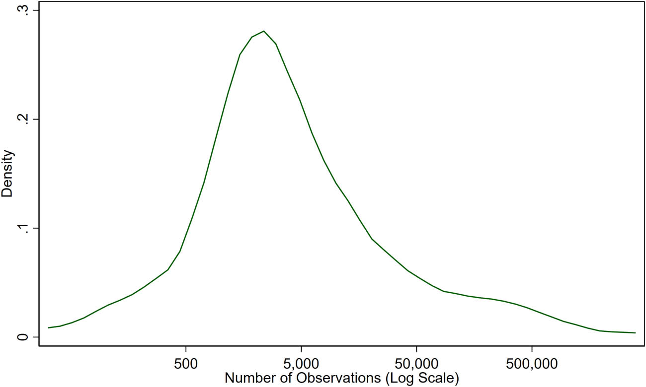
Distribution of sample sizes included in 60 top and recent articles on scholar.google.com.
Sample sizes for 30 top and 30 recent RD papers
| “Top” articles | “Recent” articles | ||
|---|---|---|---|
| Authors (Date) | Full sample size | Authors (Date) | Full sample size |
| Ludwig and Miller (2007) | 3,105 | Abou-Chadi and Krause (2018) | 391 |
| Pettersson and Lidbom (2008) | 5,913 | Anderson, Dobkin, and Gorry (2020) | 132 |
| Jacob and Lefgren (2004) | 13,687 | Goulden, Rowe, Abrahamowicz, Strumpf, and Tamblyn (2021) | 84,624 |
| Battistin, Brugiavini, Rettore, and Weber (2009) | 11,278 | Chen, Li, Kaufman, Wang, et al. (2018) | 3,653 |
| Flammer (2015) | 2,729 | Al-Awlaqi, Aamer, and Habtoor (2021) | 1,330 |
| Bronzini and Iachine (2014) | 357 | Cooray, Aida, Watt, Tsakos, et al. (2020) | 7,161 |
| Lalive (2007) | 9,734 | Zhanga, Meng, and Tian (2020) | 300 |
| Cellini, Ferrerira, and Rothstein (2010) | 6,970 | Fox, Rosen, Venkataramani, Tanser, et al. (2017) | 11,306 |
| Pellegrini, Terribile, Tarola, Muccigrosso, and Busillo (2013) | 190 | Wueppera, Wimmer, and Sauer (2020) | 2,325 |
| Ozier (2018) | 3,306 | Figlio, Holden, and Ozez (2021) | 162,887 |
| Lemieux and Milligan (2008) | 22,511 | Li, Li, Lu, and Xie (2020) | 61,849 |
| Meng (2013) | 1,946 | Takaku and Yokoyama (2021) | 15,836 |
| Van der Klaauw (2002) | 2,225 | Alonso and Andrews (2020) | 1,186 |
| Mealli and Rampichini (2012) | 299 | Khera, Wang, Nasir, Lin, and Krumholz (2019) | 195,360 |
| Berk and Rauma (1983) | 1,053 | Powdthavee (2020) | 26,315 |
| Chang, Hong, and Liskovich (2014) | 198,551 | Coyne, Oldham, Dougherty, Leonard, et al. (2018) | 678 |
| Hahn, Todd, and Van der Klaauw (1999) | 1,182 | Gonzalez (2021) | 2,039 |
| Almond and Doyle (2011) | 2,101,500 | Tymejczyk , Brazier, Yiannoutsos, Vinikoor, et al. (2019) | 17,396 |
| Urquiola and Verhoogen (2009) | 1,623 | Chen, Sudharsanan, Huang, Liu, et al. (2019) | 3,899 |
| Stancanelli and Van Soest (2012) | 1,043 | Chen, Geldsetzer, BÃďrnighausen (2020) | 5,990 |
| Mazzonna (2012) | 4,203 | ArtÃľs and Jurado (2018) | 5,871 |
| Stancanelli and Van Soest (2012) | 8,705 | Bommer, Horn, and Vollmer (2020) | 1,734 |
| Coviello and Mariniello (2012) | 17,512 | Losinski, Parks Ennis, Shaw, and Gage (2021) | 60 |
| Benavente, Crespi, and Maffioli (2007) | 1,531 | Kim and Kawachi (2020) | 2,539 |
| Calcagno and Long (2008) | 96,724 | Van Hauwaert and Huber (2020) | 3,023 |
| Bauhoff, Hotchkiss, and Smith (2011) | 5,228 | Shino and Bender (2020) | 1,313 |
| Tatsiramos, Muccigrosso, and Busillk (2013) | 2,241 | Bosch and Schady (2019) | 375,900 |
| Caliendo, Tatsiramos, and Uhlendorff (2013) | 596 | Abidi and Miquel-Flores (2018) | 1,310 |
| Malenko and Shen (2016) | 2,020 | Flammer and Bansel (2017) | 808 |
| Moss and Yeaton (2006) | 1,473 | Wang, Yi, and Li (2019) | 2,988 |
Notes: Full citation information is available upon request. See the main text for description about how we identified these 60 articles. Although we made our best efforts to identify the full sample size in the first RD estimate shown in a table in these articles, some authors were not fully clear about the sample size, and thus, we made judicious interpretations where necessary and excluded articles where we were not reasonably certain of the answer.
Simulation results for the LM1 DGP
| Conventional RDTE | Bias-corrected RDTE | |||||||||
|---|---|---|---|---|---|---|---|---|---|---|
| Sample size | Kernel | Method | RMSE | Coverage rate | RMSE | Coverage rate | ||||
| 500 | Triangular | CCT | 0.094 | 0.872 | 0.091 | 0.924 | ||||
| PLCW | 0.079 | ✓ | 0.926 | 0.088 | ✓ | 0.918 | ||||
| LR | 0.082 | 0.946 | ✓✓ | 0.089 | 0.940 | ✓ | ||||
| Uniform | CCT | 0.097 | 0.882 | 0.093 | 0.920 | |||||
| PLCW | 0.079 | 0.920 | 0.088 | 0.932 | ||||||
| LR | 0.078 | ✓✓ | 0.958 | ✓ | 0.086 | ✓✓ | 0.952 | ✓✓ | ||
| 5,000 | Triangular | CCT | 0.037 | 0.866 | 0.032 | 0.952 | ||||
| PLCW | 0.028 | ✓ | 0.902 | 0.027 | ✓ | 0.950 | ✓✓ | |||
| LR | 0.028 | 0.936 | ✓ | 0.028 | 0.958 | |||||
| Uniform | CCT | 0.037 | 0.872 | 0.033 | 0.946 | |||||
| PLCW | 0.027 | ✓✓ | 0.916 | 0.027 | 0.952 | ✓ | ||||
| LR | 0.027 | 0.942 | ✓✓ | 0.026 | ✓✓ | 0.962 | ||||
| 50,000 | Triangular | CCT | 0.014 | 0.900 | 0.013 | 0.956 | ✓ | |||
| PLCW | 0.009 | ✓ | 0.918 | 0.009 | ✓ | 0.936 | ||||
| LR | 0.009 | 0.952 | ✓✓ | 0.009 | 0.940 | |||||
| Uniform | CCT | 0.015 | 0.916 | 0.013 | 0.964 | |||||
| PLCW | 0.009 | 0.918 | 0.009 | ✓✓ | 0.948 | |||||
| LR | 0.009 | ✓✓ | 0.946 | ✓ | 0.009 | 0.950 | ✓✓ | |||
| Results | Triangular | CCT | 0.048 | 0.879 | 0.045 | 0.944 | ||||
| above | PLCW | 0.039 | ✓ | 0.915 | 0.041 | ✓ | 0.935 | |||
| averaged | LR | 0.040 | 0.945 | ✓ | 0.042 | 0.946 | ✓✓ | |||
| Uniform | CCT | 0.050 | 0.890 | 0.046 | 0.943 | |||||
| PLCW | 0.038 | 0.918 | 0.041 | 0.944 | ||||||
| LR | 0.038 | ✓✓ | 0.949 | ✓✓ | 0.040 | ✓✓ | 0.955 | ✓ | ||
| Relative | PLCW(ct)/CCT(ct) | 0.800 | PLCW(bt)/CCT(bt) | 0.912 | ||||||
| performance | LR(cu)/CCT(ct) | 0.790 | LR(bu)/CCT(bt) | 0.891 | ||||||
| LR(cu)/PLCW(ct) | 0.987 | LR(bu)/PLCW(bt) | 0.977 | |||||||
| LR(cu)/CCT(bt) | 0.838 | |||||||||
| LR(cu)/PLCW(bt) | 0.919 | |||||||||
Notes: The CCT rows show the results assuming a linear regression using CCT’s optimal bandwidth selection method applied to a linear specification. PLCW rows use PLCW’s method for polynomial order selection assuming CCT’s optimal bandwidth. LR rows use our approach of bootstrap aggregation of the PLCW method. The coverage rates are computed assuming conventional standard errors for the conventional RDTE estimates and robust standard errors for the bias-corrected results. Single check marks denote the specification that has the lowest RMSE or coverage rate closest to 0.95 within sample size and kernel across the three methods, and double check marks denote the best performance within sample size across the six
Simulation results for the L2 DGP
| Conventional RDTE | Bias-corrected RDTE | |||||||||
|---|---|---|---|---|---|---|---|---|---|---|
| Sample size | Kernel | Method | RMSE | Coverage rate | RMSE | Coverage rate | ||||
| 500 | Triangular | CCT | 0.553 | 0.934 | 0.692 | 0.932 | ||||
| PLCW | 0.404 | ✓ | 0.944 | ✓✓ | 0.527 | ✓ | 0.934 | ✓ | ||
| LR | 0.473 | 0.982 | 0.577 | 0.972 | ||||||
| Uniform | CCT | 0.541 | 0.942 | 0.646 | 0.936 | |||||
| PLCW | 0.396 | ✓✓ | 0.956 | ✓✓ | 0.488 | ✓✓ | 0.952 | ✓✓ | ||
| LR | 0.431 | 0.990 | 0.512 | 0.988 | ||||||
| 5,000 | Triangular | CCT | 0.173 | 0.924 | 0.200 | 0.942 | ✓✓ | |||
| PLCW | 0.141 | ✓✓ | 0.872 | 0.161 | ✓ | 0.938 | ||||
| LR | 0.155 | 0.954 | ✓✓ | 0.173 | 0.966 | |||||
| Uniform | CCT | 0.168 | 0.944 | ✓ | 0.194 | 0.94 | ✓ | |||
| PLCW | 0.144 | ✓ | 0.900 | 0.158 | ✓✓ | 0.934 | ||||
| LR | 0.148 | 0.962 | 0.162 | 0.968 | ||||||
| 50,000 | Triangular | CCT | 0.061 | ✓ | 0.896 | ✓ | 0.064 | 0.932 | ✓ | |
| PLCW | 0.066 | 0.736 | 0.056 | ✓✓ | 0.900 | |||||
| LR | 0.064 | 0.892 | 0.059 | 0.930 | ||||||
| Uniform | CCT | 0.060 | ✓✓ | 0.902 | 0.064 | 0.936 | ||||
| PLCW | 0.066 | 0.778 | 0.059 | 0.900 | ||||||
| LR | 0.062 | 0.908 | ✓✓ | 0.058 | ✓ | 0.944 | ✓✓ | |||
| Results | Triangular | CCT | 0.262 | 0.918 | 0.319 | 0.935 | ||||
| above | PLCW | 0.204 | ✓ | 0.851 | 0.248 | ✓ | 0.924 | |||
| averaged | LR | 0.231 | 0.943 | ✓ | 0.269 | 0.956 | ✓✓ | |||
| Uniform | CCT | 0.256 | 0.929 | 0.301 | 0.937 | ✓ | ||||
| PLCW | 0.202 | ✓✓ | 0.878 | 0.235 | ✓✓ | 0.929 | ||||
| LR | 0.214 | 0.953 | ✓✓ | 0.244 | 0.967 | |||||
| Relative | PLCW(ct)/CCT(ct) | 0.778 | PLCW(bt)/CCT(bt) | 0.778 | ||||||
| performance | LR(cu)/CCT(ct) | 0.816 | LR(bu)/CCT(bt) | 0.766 | ||||||
| LR(cu)/PLCW(ct) | 1.049 | LR(bu)/PLCW(bt) | 0.984 | |||||||
| LR(cu)/CCT(bt) | 0.671 | |||||||||
| LR(cu)/PLCW(bt) | 0.862 | |||||||||
Notes: The CCT rows show the results assuming a linear regression using CCT’s optimal bandwidth selection method applied to a linear specification. PLCW rows use PLCW’s method for polynomial order selection assuming CCT’s optimal bandwidth. LR rows use our approach of bootstrap aggregation of the PLCW method. The coverage rates are computed assuming conventional standard errors for the conventional RDTE estimates and robust standard errors for the bias-corrected results. Single check marks denote the specification that has the lowest RMSE or coverage rate closest to 0.95 within sample size and kernel across the three methods, and double check marks denote the best performance within sample size across the six
Simulation results for the LM2 DGP
| Conventional RDTE | Bias-corrected RDTE | |||||||||
|---|---|---|---|---|---|---|---|---|---|---|
| Sample size | Kernel | Method | RMSE | Coverage rate | RMSE | Coverage rate | ||||
| 500 | Triangular | CCT | 0.613 | ✓ | 0.906 | 0.679 | 0.918 | |||
| PLCW | 0.668 | 0.816 | 0.625 | ✓ | 0.886 | |||||
| LR | 0.643 | 0.912 | ✓ | 0.641 | 0.934 | ✓ | ||||
| Uniform | CCT | 0.608 | ✓✓ | 0.902 | 0.657 | 0.930 | ||||
| PLCW | 0.685 | 0.788 | 0.633 | 0.900 | ||||||
| LR | 0.622 | 0.928 | ✓✓ | 0.617 | ✓✓ | 0.944 | ✓✓ | |||
| 5,000 | Triangular | CCT | 0.226 | ✓ | 0.878 | 0.223 | ✓ | 0.944 | ||
| PLCW | 0.228 | 0.876 | 0.224 | 0.944 | ||||||
| LR | 0.226 | 0.926 | ✓ | 0.229 | 0.952 | ✓✓ | ||||
| Uniform | CCT | 0.233 | 0.864 | 0.222 | 0.936 | |||||
| PLCW | 0.232 | 0.870 | 0.223 | 0.932 | ||||||
| LR | 0.220 | ✓✓ | 0.946 | ✓✓ | 0.219 | ✓✓ | 0.962 | ✓ | ||
| 50,000 | Triangular | CCT | 0.090 | 0.864 | 0.085 | 0.928 | ||||
| PLCW | 0.075 | ✓✓ | 0.918 | 0.078 | ✓ | 0.930 | ||||
| LR | 0.076 | 0.954 | ✓ | 0.080 | 0.942 | ✓ | ||||
| Uniform | CCT | 0.093 | 0.854 | 0.087 | 0.934 | |||||
| PLCW | 0.077 | 0.918 | 0.077 | ✓✓ | 0.950 | ✓✓ | ||||
| LR | 0.076 | ✓ | 0.950 | ✓✓ | 0.077 | 0.954 | ||||
| Results | Triangular | CCT | 0.310 | ✓ | 0.883 | 0.329 | 0.930 | |||
| above | PLCW | 0.324 | 0.870 | 0.309 | ✓ | 0.920 | ||||
| averaged | LR | 0.315 | 0.931 | ✓ | 0.317 | 0.943 | ✓ | |||
| Uniform | CCT | 0.311 | 0.874 | 0.322 | 0.933 | |||||
| PLCW | 0.332 | 0.859 | 0.311 | 0.927 | ||||||
| LR | 0.306 | ✓✓ | 0.941 | ✓✓ | 0.305 | ✓✓ | 0.953 | ✓✓ | ||
| Relative | PLCW(ct)/CCT(ct) | 1.046 | PLCW(bt)/CCT(bt) | 0.940 | ||||||
| performance | LR(cu)/CCT(ct) | 0.988 | LR(bu)/CCT(bt) | 0.927 | ||||||
| LR(cu)/PLCW(ct) | 0.945 | LR(bu)/PLCW(bt) | 0.986 | |||||||
| LR(cu)/CCT(bt) | 0.930 | |||||||||
| LR(cu)/PLCW(bt) | 0.990 | |||||||||
Notes: The CCT rows show the results assuming a linear regression using CCT’s optimal bandwidth selection method applied to a linear specification. PLCW rows use PLCW’s method for polynomial order selection assuming CCT’s optimal bandwidth. LR rows use our approach of bootstrap aggregation of the PLCW method. The coverage rates are computed assuming conventional standard errors for the conventional RDTE estimates and robust standard errors for the bias-corrected results. Single check marks denote the specification that has the lowest RMSE or coverage rate closest to 0.95 within sample size and kernel across the three methods, and double check marks denote the best performance within sample size across the six
Simulation results for the J1 DGP
| Conventional RDTE | Bias-corrected RDTE | |||||||||
|---|---|---|---|---|---|---|---|---|---|---|
| Sample size | Kernel | Method | RMSE | Coverage rate | RMSE | Coverage rate | ||||
| 500 | Triangular | CCT | 2.744 | ✓ | 0.942 | 3.453 | 0.934 | |||
| PLCW | 2.844 | 0.872 | 2.973 | ✓ | 0.944 | ✓ | ||||
| LR | 2.826 | 0.946 | ✓ | 3.192 | 0.960 | |||||
| Uniform | CCT | 2.649 | ✓✓ | 0.952 | ✓✓ | 3.270 | 0.940 | |||
| PLCW | 2.845 | 0.894 | 2.840 | ✓✓ | 0.946 | ✓✓ | ||||
| LR | 2.706 | 0.970 | 2.928 | 0.974 | ||||||
| 5,000 | Triangular | CCT | 0.866 | ✓ | 0.930 | 0.903 | 0.962 | ✓ | ||
| PLCW | 0.868 | 0.930 | 0.892 | ✓ | 0.962 | ✓ | ||||
| LR | 0.952 | 0.968 | ✓ | 0.920 | 0.964 | |||||
| Uniform | CCT | 0.838 | ✓✓ | 0.948 | ✓✓ | 0.892 | 0.952 | ✓✓ | ||
| PLCW | 0.845 | 0.948 | ✓✓ | 0.883 | 0.958 | |||||
| LR | 0.884 | 0.976 | 0.878 | ✓✓ | 0.978 | |||||
| 50,000 | Triangular | CCT | 0.294 | ✓✓ | 0.920 | 0.303 | ✓ | 0.950 | ✓✓ | |
| PLCW | 0.300 | 0.916 | 0.303 | 0.950 | ✓✓ | |||||
| LR | 0.315 | 0.944 | ✓ | 0.323 | 0.968 | |||||
| Uniform | CCT | 0.298 | ✓ | 0.914 | 0.292 | ✓✓ | 0.950 | ✓✓ | ||
| PLCW | 0.304 | 0.916 | 0.293 | 0.948 | ||||||
| LR | 0.305 | 0.950 | ✓✓ | 0.298 | 0.972 | |||||
| Results | Triangular | CCT | 1.302 | ✓ | 0.931 | 1.553 | 0.949 | ✓ | ||
| above | PLCW | 1.337 | 0.906 | 1.390 | ✓ | 0.952 | ||||
| averaged | LR | 1.364 | 0.953 | ✓✓ | 1.479 | 0.964 | ||||
| Uniform | CCT | 1.262 | ✓✓ | 0.938 | ✓ | 1.484 | 0.947 | |||
| PLCW | 1.331 | 0.919 | 1.339 | ✓✓ | 0.951 | ✓✓ | ||||
| LR | 1.298 | 0.965 | 1.368 | 0.975 | ||||||
| Relative | PLCW(ct)/CCT(ct) | 1.028 | PLCW(bt)/CCT(bt) | 0.895 | ||||||
| performance | LR(cu)/CCT(ct) | 0.998 | LR(bu)/CCT(bt) | 0.881 | ||||||
| LR(cu)/PLCW(ct) | 0.971 | LR(bu)/PLCW(bt) | 0.985 | |||||||
| LR(cu)/CCT(bt) | 0.836 | |||||||||
| LR(cu)/PLCW(bt) | 0.934 | |||||||||
Notes: The CCT rows show the results assuming a linear regression using CCT’s optimal bandwidth selection method applied to a linear specification. PLCW rows use PLCW’s method for polynomial order selection assuming CCT’s optimal bandwidth. LR rows use our approach of bootstrap aggregation of the PLCW method. The coverage rates are computed assuming conventional standard errors for the conventional RDTE estimates and robust standard errors for the bias-corrected results. Single check marks denote the specification that has the lowest RMSE or coverage rate closest to 0.95 within sample size and kernel across the three methods, and double check marks denote the best performance within sample size across the six
References
[1] Efron B. Estimation and accuracy after model selection. J Amer Stat Assoc. 2014 Oct;109(507):991–1007. 10.1080/01621459.2013.823775. Search in Google Scholar PubMed PubMed Central
[2] Imbens G, Kalyanaraman K. Optimal bandwidth choice for the regression discontinuity estimator. Rev Econ Stud. 2012 Nov;79(3):933–59. 10.1093/restud/rdr043. Search in Google Scholar
[3] Calonico S, Cattaneo MD, Titiunik R. Robust nonparametric confidence intervals for regression-discontinuity designs. Econometrica. 2014 Nov;82(6):2295–326. https://www.jstor.org/stable/43616914. 10.3982/ECTA11757Search in Google Scholar
[4] Pei Z, Lee DS, Card D, Weber A. Local polynomial order in regression discontinuity designs. J Business Econ Stat. 2021 Jun;40(3):1259–67. 10.1080/07350015.2021.1920961. Search in Google Scholar
[5] Thistlethwaite DL, Campbell DT. Regression-discontinuity analysis: An alternative to the ex post facto experiment. J Educ Psychol. 1960 51(6):309–17. 10.1037/h0044319. Search in Google Scholar
[6] Hahn J, Todd P, Van der Klaauw W. Identification and estimation of treatment effects with a regression-discontinuity design. Econometrica. 2001 Sep;69(1):201–9. 10.1111/1468-0262.00183. Search in Google Scholar
[7] Cattaneo MD, Titiunik R. Regression discontinuity designs. Ann Rev Econ. 2022 14:821–51. 10.1146/annurev-economics-051520-021409. Search in Google Scholar
[8] Imbens GW, Lemieux T. Regression discontinuity designs: A guide to practice. J Econ. 2008 Feb;142(2):615–35. 10.1016/j.jeconom.2007.05.001. Search in Google Scholar
[9] Cattaneo M, Idrobo N, Titiunik R. A practical introduction to regression discontinuity designs: foundations (elements in quantitative and computational methods for the social sciences). Cambridge: Cambridge University Press; 2020. 10.1017/9781108684606. Search in Google Scholar
[10] Cattaneo M, Idrobo N, Titiunik R. A practical introduction to regression discontinuity designs: extensions (elements in quantitative and computational methods for the social sciences). Cambridge: Cambridge University Press; 2020. 10.1017/9781108684606. Search in Google Scholar
[11] Nichols A. rd 2.0: Revised Stata module for regression discontinuity estimation. 2011. http://ideas.repec.org/c/boc/bocode/s456888.html. Search in Google Scholar
[12] Calonico S, Cattaneo MD, Titiunik R. Robust data-driven inference in the regression-discontinuity design. Stata J. 2014 Dec;14(4):909–46. 10.1177/1536867X1401400413. Search in Google Scholar
[13] Calonico S, Cattaneo MD, Farrell MH. Optimal bandwidth choice for robust bias-corrected inference in regression discontinuity designs. Econ J. 2020 Nov;23(2):192–210. 10.1093/ectj/utz022. Search in Google Scholar
[14] Calonico S, Cattaneo MD, Farrell MH, Titiunik R. RDROBUST: Stata module to provide robust data-driven inference in the regression-discontinuity design. 2018. https://ideas.repec.org/c/boc/bocode/s458483.html. Search in Google Scholar
[15] Calonico S, Cattaneo MD, Farrell MH. On the effect of bias estimation on coverage accuracy in nonparametric inference. J Amer Stat Assoc. 2018 Mar;113(522):767–79, 10.1080/01621459.2017.1285776. Search in Google Scholar
[16] Calonico S, Cattaneo MD, Farrell MH. Coverage error optimal confidence intervals for local polynomial regression. Bernoulli. 2022 Nov;28(4):2998–3022. 10.3150/21-BEJ1445. Search in Google Scholar
[17] Gelman A, Imbens G. Why high-order polynomials should not be used in regression discontinuity designs, J Business Econ Stat. 2019 May;37(3):447–56. 10.1080/07350015.2017.1366909. Search in Google Scholar
[18] Breiman L. Bagging predictors. Machine Learn. 1996;24:123–40. 10.1007/BF00058655. Search in Google Scholar
[19] Steel MFJ. Model averaging and its use in economics. J Econ Literature. 2020 Sep;58(3):644–719. 10.1257/jel.20191385. Search in Google Scholar
[20] Hjort NL, Claeskens G. Frequentist model average estimators. J Amer Stat Assoc. 2003 Dec;98(464):879–99. 10.1198/016214503000000828. Search in Google Scholar
[21] Otávio B, Gray C, Yang H. Bootstrap confidence intervals for sharp regression discontinuity designs with the uniform kernel. In: Cattaneo MD, Escanciano JC, editors. Advances in econometrics: Regression discontinuity designs: theory and applications. Bingley: Emerald Publishing; 2017. Search in Google Scholar
[22] Chiang HD, Hsu Y, Sasaki Y. Robust uniform inference for quantile treatment effects in regression discontinuity designs. J Econ. 2019 Aug;211(2):589–618. 10.1016/j.jeconom.2019.03.006. Search in Google Scholar
[23] Chiang HD, Sasaki Y. Causal inference by quantile regression kink designs. J Econ. 2019 Jun;210(2):405–33. 10.1016/j.jeconom.2019.02.005. Search in Google Scholar
[24] Efron B. Bootstrap methods: Another look at the jackknife. Ann Stat. 1979;7:1–26. 10.1007/978-1-4612-4380-9_41. Search in Google Scholar
[25] Dima C. 2013 Why not report the mean of a bootstrap distribution? Answer. Accessed on December 23, 2012 from https://stats.stackexchange.com/questions/71357/why-not-report-the-mean-of-a-bootstrap-distribution. Search in Google Scholar
[26] Cheng M, Fan J, Marron JS. On automatic boundary corrections. Ann Stat. 1997 Aug;25(4):1691–708. http://dx.doi.org/10.1214/aos/1031594737. Search in Google Scholar
[27] Lee DS. Randomized experiments from non-random selection in U.S. house elections. J Econometr. 2008 Feb;142(2):675–97. 10.1016/j.jeconom.2007.05.004. Search in Google Scholar
[28] Ludwig J, Miller DL. Does head start improve children’s life chances? Evidence from a regression discontinuity design. Quarter J Econom. 2007 Feb;122(1):159–208. https://www.jstor.org/stable/25098840. 10.1162/qjec.122.1.159Search in Google Scholar
[29] Jacob R, Zhu P, Somers M, Bloom H. A practical guide to regression discontinuity. MDRC. 2012. http://www.mdrc.org/sites/default/files/regression_discontinuity_full.pdf. Search in Google Scholar
[30] Card D, Lee DS, Pei Z, Weber A. Inference on causal effects in a generalized regression kink design. Econometrica. 2015 Dec;83(6):2453–83. 10.3982/ECTA11224. Search in Google Scholar
[31] Van Kerm P. Adaptive kernel density estimation. Stata J. 2002 3(2):148–56. 10.1177/1536867X0300300204. Search in Google Scholar
© 2024 the author(s), published by De Gruyter
This work is licensed under the Creative Commons Attribution 4.0 International License.
Articles in the same Issue
- Research Articles
- Evaluating Boolean relationships in Configurational Comparative Methods
- Doubly weighted M-estimation for nonrandom assignment and missing outcomes
- Regression(s) discontinuity: Using bootstrap aggregation to yield estimates of RD treatment effects
- Energy balancing of covariate distributions
- A phenomenological account for causality in terms of elementary actions
- Nonparametric estimation of conditional incremental effects
- Conditional generative adversarial networks for individualized causal mediation analysis
- Mediation analyses for the effect of antibodies in vaccination
- Sharp bounds for causal effects based on Ding and VanderWeele's sensitivity parameters
- Detecting treatment interference under K-nearest-neighbors interference
- Bias formulas for violations of proximal identification assumptions in a linear structural equation model
- Current philosophical perspectives on drug approval in the real world
- Foundations of causal discovery on groups of variables
- Improved sensitivity bounds for mediation under unmeasured mediator–outcome confounding
- Potential outcomes and decision-theoretic foundations for statistical causality: Response to Richardson and Robins
- Quantifying the quality of configurational causal models
- Design-based RCT estimators and central limit theorems for baseline subgroup and related analyses
- An optimal transport approach to estimating causal effects via nonlinear difference-in-differences
- Estimation of network treatment effects with non-ignorable missing confounders
- Double machine learning and design in batch adaptive experiments
- The functional average treatment effect
- An approach to nonparametric inference on the causal dose–response function
- Review Article
- Comparison of open-source software for producing directed acyclic graphs
- Special Issue on Neyman (1923) and its influences on causal inference
- Optimal allocation of sample size for randomization-based inference from 2K factorial designs
- Direct, indirect, and interaction effects based on principal stratification with a binary mediator
- Interactive identification of individuals with positive treatment effect while controlling false discoveries
- Neyman meets causal machine learning: Experimental evaluation of individualized treatment rules
- From urn models to box models: Making Neyman's (1923) insights accessible
- Prospective and retrospective causal inferences based on the potential outcome framework
- Causal inference with textual data: A quasi-experimental design assessing the association between author metadata and acceptance among ICLR submissions from 2017 to 2022
- Some theoretical foundations for the design and analysis of randomized experiments